Sea Ice Monitoring with CFOSAT Scatterometer Measurements Using Random Forest Classifier

Abstract

The Ku-band scatterometer called CSCAT onboard the Chinese–French Oceanography Satellite (CFOSAT) is the first spaceborne rotating fan-beam scatterometer (RFSCAT). This paper performs sea ice monitoring with the CSCAT backscatter measurements in polar areas. The CSCAT measurements have the characteristics of diverse incidence and azimuth angles and separation between open water and sea ice. Hence, five microwave feature parameters, which show different sensitivity to ice or water, are defined and derived from the CSCAT measurements firstly. Then the random forest classifier is selected for sea ice monitoring because of its high overall accuracy of 99.66% and 93.31% in the Arctic and Antarctic, respectively. The difference of features ranked by importance in different seasons and regions shows that the combination of these parameters is effective in discriminating sea ice from water under various conditions. The performance of the algorithm is validated against the sea ice edge data from the EUMETSAT Ocean and Sea Ice Satellite Application Facility (OSI SAF) on a global scale in a period from 1 January 2019 to 10 May 2021. The mean sea ice area differences between CSCAT and OSI SAF product in the Arctic and Antarctic are 0.2673 million km² and −0.4446 million km², respectively, and the sea ice area relative errors of CSCAT are less than 10% except for summer season in both poles. However, the overall sea ice area derived from CSCAT is lower than the OSI SAF sea ice area in summer. This may be because the CSCAT is trained by radiometer sea ice concentration data while the radiometer measurement of sea ice is significantly affected by melting in the summer season. In conclusion, this research verifies the capability of CSCAT in monitoring polar sea ice using a machine learning-aided random forest classifier. This presented work can give guidance to sea ice monitoring with radar backscatter measurements from other spaceborne scatterometers, particular for the recently launched FY-3E scatterometer (called WindRad).

1. Introduction

Polar sea ice, as an important input to the global climate model and a sensitive indicator of climate change, has always been paid attention by climate researchers [1,2]. Sea ice forms a new interface between the upper ocean and the lower atmosphere, which can change the radiation and energy balance of the ocean surface and isolate the heat exchange and water vapor exchange between the ocean and the atmosphere by blocking the wind field’s momentum input to the ocean [3]. In addition, sea ice with high albedo can reduce the absorption of solar radiation [4]. The freezing and thawing process of sea ice will also affect the ocean thermohaline circulation, further affecting the redistribution of marine life [5]. Therefore, sea ice modulates the atmosphere–ocean interaction by influencing the exchange of matter and energy, ocean surface albedo, ocean temperature, and salinity circulation, and thus has a significant impact on global climate [6].

The traditional sea ice monitoring method is mainly carried out by artificial field observation, which is time-consuming and laborious with limited coverage. Satellite-based microwave sensors, however, have become the most effective means of sea ice monitoring and ice condition assessment with their advantages of being all-weather, near real-time, large-scale, and having capability for long-term continuous observation [7,8,9]. Detection of sea ice extent is generally performed by two types of sensors, that is, the passive microwave radiometer [10,11,12] and the active microwave scatterometer [13]. The radiometer observes emissions from the Earth’s surface and can provide sea ice concentration within each pixel, which is considered the main source for sea ice mapping. The limitation is the high sensitivity to atmospheric effects and the difficulty in detecting sea ice in summer. The scatterometer sends a microwave signal toward the Earth’s surface and records the returned signal. It has been verified as a useful tool for polar sea ice detection such as sea ice extent [14,15,16], type [17,18,19], and motion [20,21]. Compared to the radiometer, the scatterometer cannot provide information on sea ice concentration, but it has higher spatial resolution and much lower sensitivity to atmospheric effects [22,23].

Table 1 summarizes the development of the existing spaceborne scatterometers and some related sea ice research. It can be seen that all European Space Agency (ESA) scatterometers operate at C-band vertical polarization with fixed fan-beam, including the active microwave instrument (AMI) onboard ERS-1 and 2 satellites and the advanced scatterometer (ASCAT) onboard the METOP-A, B, and C satellites. The group at IFREMER (French Institute for Marine Development) firstly used C-band ERS/AMI data for sea ice detection [24,25]. Two parameters, that is, the anisotropy coefficient, anis, and the change of backscatter with incidence angle, dsigma, were first proposed for water and ice discrimination. Breivik et al. proposed a new parameter combining the properties of anis and dsigma, that is, anisFMB, where the measurements from three antennas sight are used [26]. This method has been validated against ice charts from the Norwegian Ice Service, indicating realistic ice edge results but with a weather-induced noise problem, where auxiliary information should be used to remove this noise. Bayesian classification based on multi-sensor parameters derived from ASCAT and SSM/I were implemented to give high-quality ice edge details, and was therefore chosen for the EUMETSAT Ocean and Sea Ice Satellite Application Facility (OSI SAF) ice edge product operational use [26,27,28]. Haan and Stoffelen constructed the three-dimensional ice Geophysical Model Function (GMF) using an ERS scatterometer [29], where the ice discrimination is based on the normalized distance to the ice line model and the distance to the wind cone model. This method has been tested using ERS-2 scatterometer data and appears to be reliable in more than 98% of cases. Belmonte et al. extended this approach and proposed Bayesian classification based on GMFs for sea ice detection with SeaWinds and ASCAT, respectively [15,16]. The performance of this method has been validated against active and passive microwave sea ice detection algorithms and high resolution optical and radar imagery, indicating that this method can provide more accurate information for the characterization of sea ice during melting season.

Table 1. Summary of spaceborne scatterometers and related sea ice studies.

Mission	ERS-1/2	ADEOS-1	QuikSCAT	METOP	OceanSAT-II	HY-2A
scatterometer	AMI	NSCAT	SeaWinds	ASCAT	OSCAT	SCAT
Date	July 1991–March 2000 April 1995–May 2011	August 1996–June 1997	June 1999– November 2009	June 2007– present	October 2009– February 2014	August 2011–November 2020
Institute	ESA	NASDA /NASA	NASA	ESA	ISRO	NSOAS
Frequency (band)	5.3 GHz (C)	13.995 GHz (Ku)	13.4 GHz (Ku)	5.3 GHz (C)	13.515 (Ku)	13.255 (Ku)
Beam type	Fixed fan-beam	Fixed fan-beam	Rotating pencil-beam	Fixed fan-beam	Rotating pencil-beam
Polarization	3VV	3VV × 2 1HH × 2	HH-inner VV-outer	3VV × 2	HH-inner VV-outer
Incidence angles	18–59°	17–60°	46°, 54.4°	25–65°	49°, 57°	41°, 48°
Viewing geometry
algorithm	Bayesian based on GMF	RL-N algorithm	Bayesian based on multi-sensor analysis, Modified RL-N algorithm	Bayesian based on multi-sensor analysis, Bayesian based on GMF	Modified RL-N algorithm	FLDA SVM
references	Cavanié et al., 1993 [24] Gohin and Cavanié, 1994 [25] Haan and Stoffelen, 2001 [29]	Remund and Long, 1999 [30]	Rivas and Stoffelen, 2011 [15] Remund and Long, 2013 [31]	Rivas et al., 2012 [16] Breivik et al., 2012 [26]	Hill and Long, 2017 [32]	Li et al., 2016 [33]

It is shown in Table 1 that National Aeronautics and Space Administration (NASA), Indian Space Research Organization (ISRO), and National Satellite Marine Application Center (NSMAC) scatterometers operate at Ku-band with dual-polarization, including ADEOS-1/NSCAT, QuikSCAT/SeaWinds, OceanSAT-II;/OSCAT, and HY-2A/SCAT. All of these scatterometers use a rotating pencil-beam, except for the NSCAT (fixed fan-beam). Remund and Long firstly proposed an algorithm for ice/water discrimination using NSCAT datasets [30]. The algorithm, known as Remund/Long-NSCAT (RL-N) algorithm, used copolarization ratio and incidence angle dependence as the primary classification parameters to distinguish water and ice. The normalized radar backscatter coefficient ${\sigma }_0$ estimate error standard deviation ($\kappa$) was used to correct the errors from linear and quadratic discrimination. The resulting sea ice edge showed good agreement with the 30% ice concentration edge derived from the NASA Team algorithm special sensor microwave imager (SSMI). Considering the differences between the NSCAT and SeaWinds instrument configurations, a modified RL-N algorithm was proposed for SeaWinds sea ice extent retrieval [31], where the parameter $\kappa$ gives more information due to its increasing sensitivity to azimuthal variations. A decade of QuikSCAT scatterometer sea ice extent data using RL-N algorithm has been automatically processed. The corresponding results were compared with sea ice concentration derived from SSMI data and RADARSAT synthetic aperture radar imagery, showing that the retrieved ice edge correlates well with 15%–30% and 0%–30% ice concentration contours derived from the NASA Team algorithm during the ice advance and retreat phases, respectively. The Modified RL-N algorithm has become the basis of operational use for SeaWinds sea ice extent products. In addition, processing of OSCAT data using the RL-N algorithm with some modifications focusing on the data gaps problem has been used to support sea ice extent mapping and to extend the SeaWinds sea ice data record [32]. The validation results show that the OSCAT derived sea ice extent falls between the SSM/I 0% and 30% sea ice concentration. Li et al. used Fisher’s linear discriminant analysis and image processing technology to map the sea ice extent based on HY-2A/SCAT data, where the combination of five parameters including polarization ratio, HH and VV polarized measurement and their corresponding daily standard deviations were verified to identify sea ice and water effectively [33]. The results show the HY-2A/SCAT ice extent falls between SSMIS NASA Team 5% and 30% ice extent.

The China–France oceanography satellite (CFOSAT), carrying a first-ever spaceborne Ku-band rotating fan-beam scatterometer (CSCAT), was launched on 29 October 2018 [34]. It is reported that the CSCAT instrument is generally stable in terms of noise measurements and internal calibration, and the CSCAT sea surface wind products are of good quality [35]. However, there are few studies on sea ice detection based on CSCAT measurements [36]. The purpose of this paper is to propose a CSCAT sea ice detection algorithm based on machine learning-aided classification methods. This paper is organized as follows. Background information about the CSCAT instrument and the datasets used for training and validation are firstly described in Section 2. The sea ice monitoring algorithm based on random forest and data processing flow are then described in Section 3. The sea ice monitoring results are presented and discussed in Section 4 and Section 5, respectively. The conclusions are finally addressed in Section 6.

2. Datasets

2.1. CFOSAT Scatterometer (CSCAT)

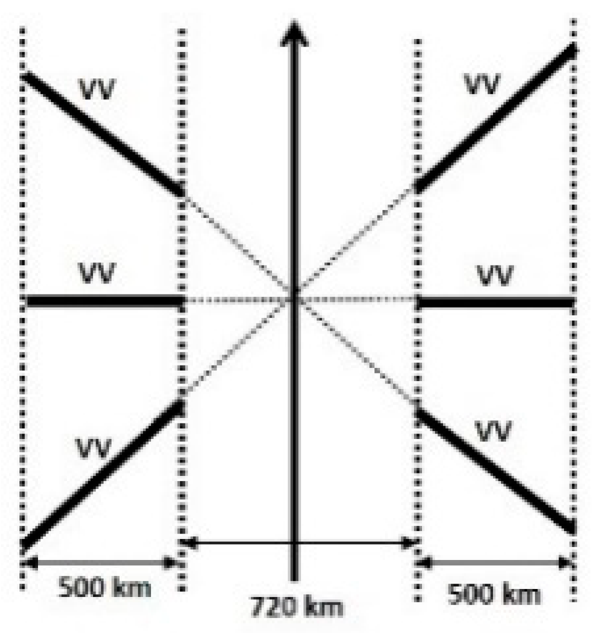
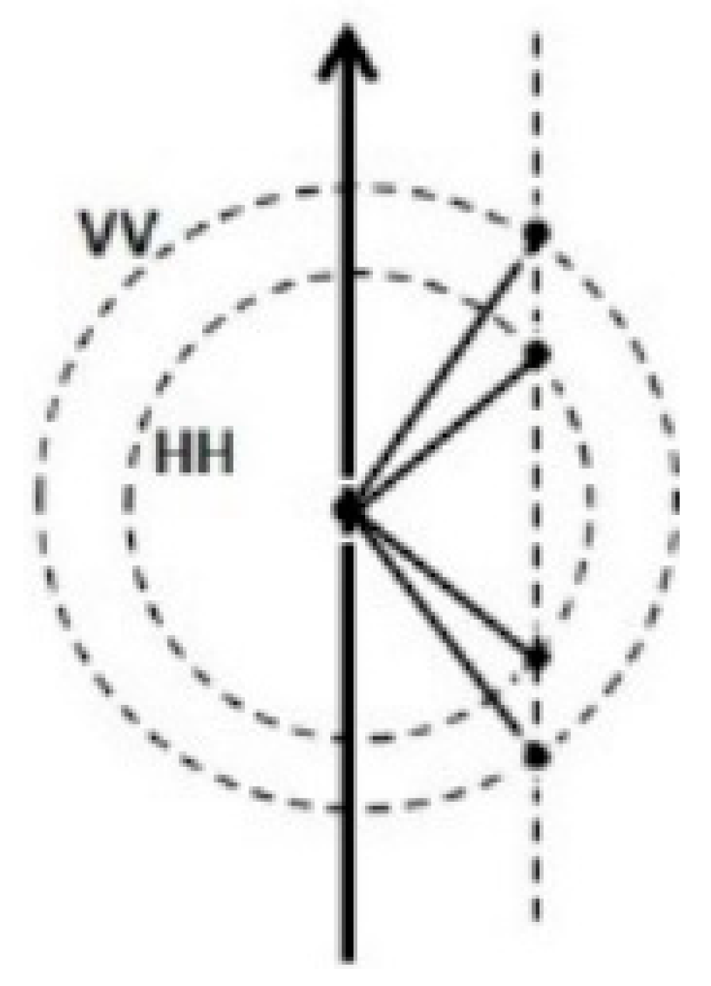
The CFOSAT satellite is in a sun-synchronous orbit with an altitude of about 520 km, an inclination of 97.5°, and a local equator-crossing time of 7:00 a.m. in descending node. The CSCAT operates in Ku-band frequency using one vertically polarized (VV) fan-beam and one horizontally polarized (HH) fan-beam antenna. Both beams observe the Earth’s surface at medium incidence angles (28~51°), and the antenna azimuths of VV and HH beams are offset by 180° to maximize the azimuth diversity which favors the sea surface wind retrieval [34]. The CSCAT transmits vertically and horizontally polarized pulses alternatively, and both of the pulse repetition rates of VV and HH beams are 75 Hz. It has a large observational swath of 1000 km so that it can provide global coverage of wind measurement in 3 days. Table 2 lists the main specifications of CSCAT [35].

Table 2. List of the main specifications of CSAT.

Obit Parameters
Orbit height	520 km
Inclination	97.5°
Orbital period	94.90 min
Descending node equatorial crossing (local time)	~07:00 a.m.
CSCAT payload parameters
Frequency	Ku (13.256 GHz)
Polarization	HH, VV
Incidence angle	28–51°
Beam type	rotating range-gated fan-beam scatterometer (RFSCAT)
Rotation speed	3.4 rpm
Pulse repetition frequency (PRF)	150 Hz
bandwidth	0.5 MHz
Pulse duration	1.35 ms
Pulse peak power	120 W
Swath	1000 km
Wind vector cells (resolution)	42 (25 km × 25 km) 84 (12.5 km × 12.5 km)

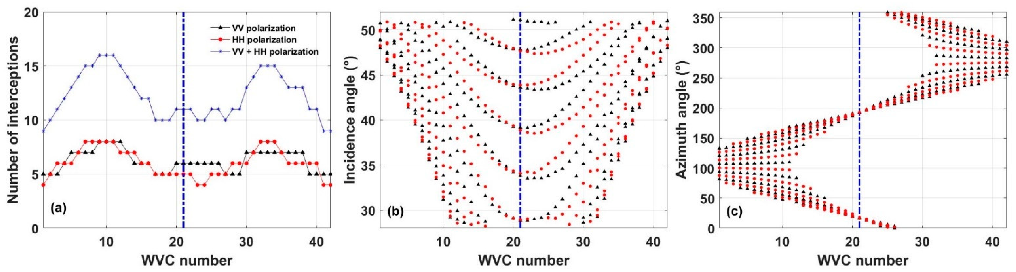
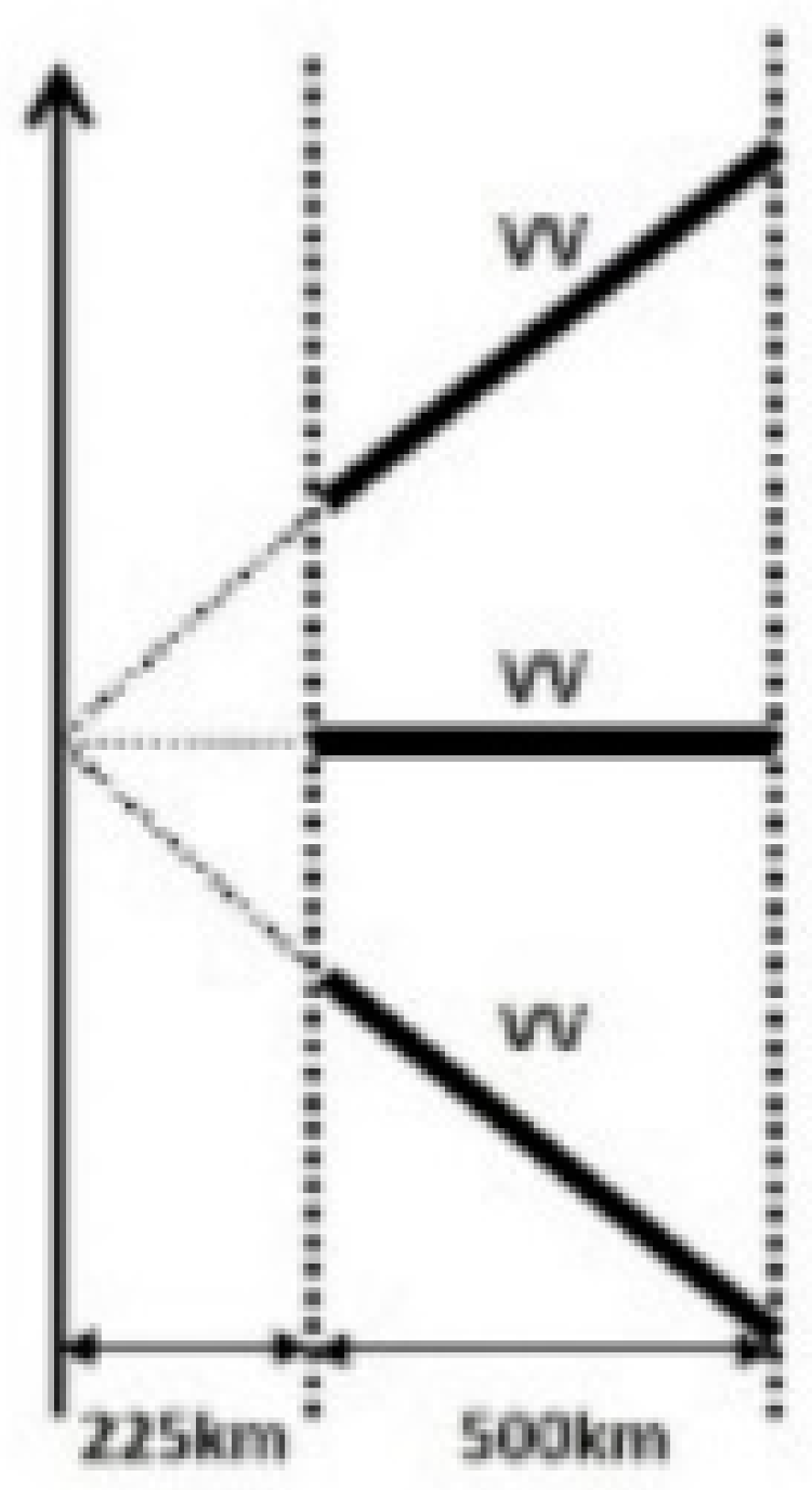
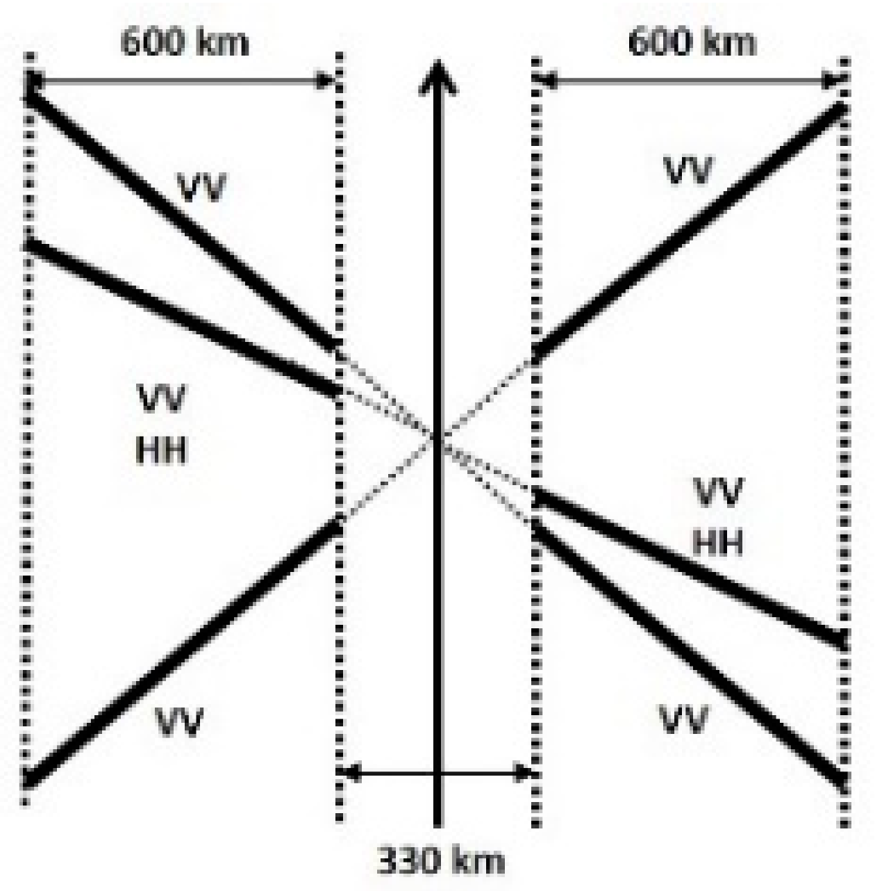
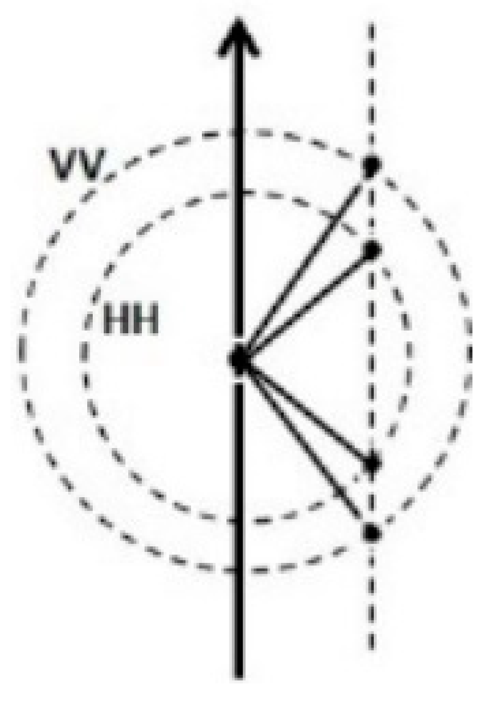
The CSCAT combines the characteristics of the fixed fan-beam and rotating pencil-beam scatterometers [34]. Specifically, it has no nadir gap compared to the fixed fan-beam scatterometer and has a larger number of ${\sigma }_0$ with diverse incidence and azimuth angles compared to the pencil-beam one. CSCAT has two kinds of wind vector cell (WVC) configurations in the 1000 km swa including 42 and 84 WVCs with sampling resolution of 25 km × 25 km and 12.5 km × 12.5 km, respectively. Figure 1 shows an example of the distribution of CSCAT WVCs for a descending row at latitude of about 20°. The WVC number is defined as the number from the leftmost to the rightmost swath. It can be seen that the incidence angle information near the satellite ground track is most abundant, but the azimuth angle is only at around $\pm {180}^{°}$ with an observation number of less than 12. The information of incidence and azimuth angles at the far end of the swath center is very little with the lowest observation number being less than 10. The observation condition at around $\pm 300$ km away from the swath center is most suitable for wind field retrieval.

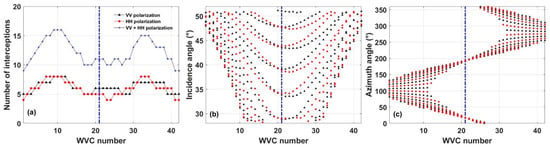
Figure 1. Distribution of CSCAT (a) number of interceptions (black triangles for VV polarization, red dots for HH polarization, and blue stars for total observation), (b) incidence, and (c) azimuth angles versus the cross-track WVC number for a descending row at latitude of ~20°, where the black triangle and red dots represent the VV and HH polarization views, respectively.

2.2. Sea Ice Class Data for Model Training

The purpose of sea ice monitoring is to distinguish sea ice from water, which can be regarded as a classification problem. A general tool for combining various feature parameters to solve the classification question has been given by a machine learning-based approach [37,38]. The machine learning classifier can be generally categorized into three aspects according to the model building process, that is, the supervised learning, the unsupervised learning, and the semi-supervised learning classifier. As for the supervised learning classifier which will be used in this study, the training datasets with labeled or priori information are necessarily needed for training a model, and the test datasets are then used to evaluate the accuracy of predictions given by the trained model.

For the training of the sea ice classification method, a reference dataset is needed. In this study, the daily National Oceanic and Atmospheric Administration/National Snow and Ice Data Center (NOAA/NSIDC) climate data record (CDR) [39] and the daily near-real-time NOAA/NSIDC climate data record (NRT CDR) of passive microwave sea ice concentration [40] are used as reference data for different temporal coverages. NOAA/NSIDC sea ice concentration is used as the training data in this paper because it has the same spatial resolution of 25 km as CSCAT data, and the data has good continuity, which can ensure the stability of a priori information acquisition of the algorithm used in this paper. The reason for using these two datasets as reference data is that the CDR datasets are only updated to 31 December 2020 right now, while the NRT CDR dataset is the daily-updated version of the CDR datasets, and it can fill the temporal gap between updates of the final CDR and offer the most recent data, which is therefore chosen as reference data during 1 January 2021–10 May 2020.

Table 3 lists the overview of CDR and NRT CDR, respectively. The major difference between these two datasets is the usage of brightness temperature data from different sources, as shown in Table 3. The used variable in this study from CDR and NRT CDR are named as “cdr _seaice_conc” and “seaice_conc_cdr”, respectively, both of which are merged from the NASA Team and NASA Bootstrap processed sea ice concentrations using the CDR algorithm. Basically, the CDR algorithm selects the higher concentration value between NASA Team and NASA Bootstrap as the output concentration. Comprehensive validation of CDR ice concentration fields has not been studied yet, but related studies concluded that the CDR and NASA Bootstrap results are quite similar in both hemispheres, while larger differences exist between the CDR and the NASA Team results [41].

Table 3. The overview of National Oceanic and Atmospheric Administration/National Snow and Ice Data Center (NOAA/NSIDC) climate data record of passive microwave sea ice concentration.

Specification	NOAA/NSIDC Climate Data Record (CDR) of Passive Microwave Sea Ice Concentration	Near-Real-Time (NRT) NOAA/NSIDC Climate Data Record (CDR) of Passive Microwave Sea Ice Concentration
Website	https://nsidc.org/data/G02202/versions/4 (accessed on 18 November 2021)	https://nsidc.org/data/G10016/versions/2 (accessed on 18 November 2021)
Used temporal coverage	1 January 2019–31 December 2019	1 January 2020–10 May 2021
Projection and grid size	Polar stereographic projection North: 304 (columns) × 448 (rows) South: 316 (columns) × 332 (rows)
Spatial coverage (over ocean area)	northern hemisphere: 31.1° N–89.84° N, 180° E–180° W southern hemisphere: 39.36° S–89.84° S, 180° E–180° W
Spatial resolution	25 km × 25 km
Used temporal resolution	1 day
Used variable name	cdr_seaice_conc	seaice_conc_cdr
Used dataset	DMSP SSM/I-SSMIS Daily Polar Gridded Brightness Temperatures (NSIDC-0001)	Near-Real-Time DMSP SSM/I-SSMIS Daily Polar Gridded Brightness Temperatures (NSIDC-0080)
Brief description of used variable	NOAA/NSIDC daily sea ice CDR	NRT NOAA/NSIDC daily sea ice CDR
Platform(s)	DMSP 5D-3/F18	DMSP 5D-3/F18
Sensor(s)	SSMIS	SSMIS

The sea ice concentration data are gridded using polar stereographic projection, where a projection plane to Earth’s surface at 70° N or 70° S is specified to minimize the distortion in the marginal ice zones. The grid cell resolution is 25 km × 25 km, the dimensions of which in the x and y directions of the projection grid centers are 304 × 448 for the northern hemisphere and 316 × 332 for the southern hemisphere, respectively [42]. It was noted that a polar orbit and wide swath provides near-complete coverage at least once per day in the polar regions except for a small region around the North Pole called the pole hole. As shown in Table 3, the SSMIS sensor is used for NSIDC sea ice concentration retrieval. For SSMIS, the pole hole is 94 km in radius and is located poleward of 89.18°N with an area of 0.029 million km². Similar to the definition of OSI SAF sea ice edge product which will be described in Section 2.3, sea ice concentrations below 40%, between 40% and 70%, and above 70% are identified as open water, open ice, and closed ice, respectively.

2.3. Validation Data

The sea ice edge product provided by OSI SAF is used as the main validation data source in this study. There are three main reasons for using the OSI SAF sea ice product as validation data. Firstly, the OSI SAF sea ice retrieval algorithm uses the same type of payload data source as the one used in this paper, that is, both scatterometer and radiometer data are used. Secondly, both of these two algorithms are supervised classification. Thirdly, the OSI SAF sea ice product has excellent temporal and spatial continuity, providing an effective data source for long-time series comparison and analysis.

Table 4 lists the correspondence between sea ice classes as used by operational sea ice services, sea ice concentration range, and the sea ice class chosen for the Ocean and Sea Ice Satellite Application Facility (OSI SAF) classification [28]. A threshold in ice concentration of 15% is often used to define sea ice extent in scientific studies and climate applications [15]. As for the OSI SAF sea ice edge retrieval, the OSI SAF ice concentration product is used as reference data, where sea ice concentration below 40%, between 40% and 70%, and above 70% are identified as open water, open ice, and closed ice, respectively.

Table 4. The correspondence between ice service sea ice class, sea ice concentration range, and OSI SAF ice edge class.

Ice Service Sea Ice Class	Sea Ice Concentration Range	OSI SAF Ice Edge Class
Open water	Less than 1/10	Open water
Very open drift ice	1/10–4/10	Open water/open ice
Open drift ice	4/10–7/10	Open ice
Closed drift ice	7/10–9/10	Closed ice
Fast ice	More than 9/10	Closed ice

OSI SAF ice classes are assigned from atmospherically corrected SSMIS brightness temperature and ASCAT backscatter values, using a multi-sensor-based Bayesian approach. Since the sea ice properties vary with the seasons, the dynamical probability density functions (PDFs) of different ice classes are continuously updated based on the training dataset from the preceding 15 days. Four parameters, including three passive microwave (PMW) parameters, PR19, GR1937, PRn90, and the ASCAT parameter aniFMB are used for the OSI SAF ice edge product [27,28]. Since the Bayesian approach describes the probability of occurrence of the most likely surface class, the probability itself can be an indicator of statistical uncertainty of the classification. The OSI SAF grid is a polar-stereographic grid with 10 km spatial resolution, the dimensions of which in the x and y directions of the projection grid centers are 760 × 1120 for the northern hemisphere and 790 × 830 for the southern hemisphere, respectively. Figure 2 gives an example of OSI SAF sea ice products on 8 April 2020, including the sea ice edge in the Arctic and Antarctic, respectively.

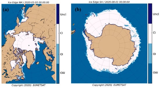
Figure 2. OSI SAF sea ice edge product in the 8 April 2020 from (a) Arctic and (b) Antarctic, respectively. Figures are accessed from https://osisaf-hl.met.no/quicklooks-1prod (accessed on 18 November 2021).

3. Methodology

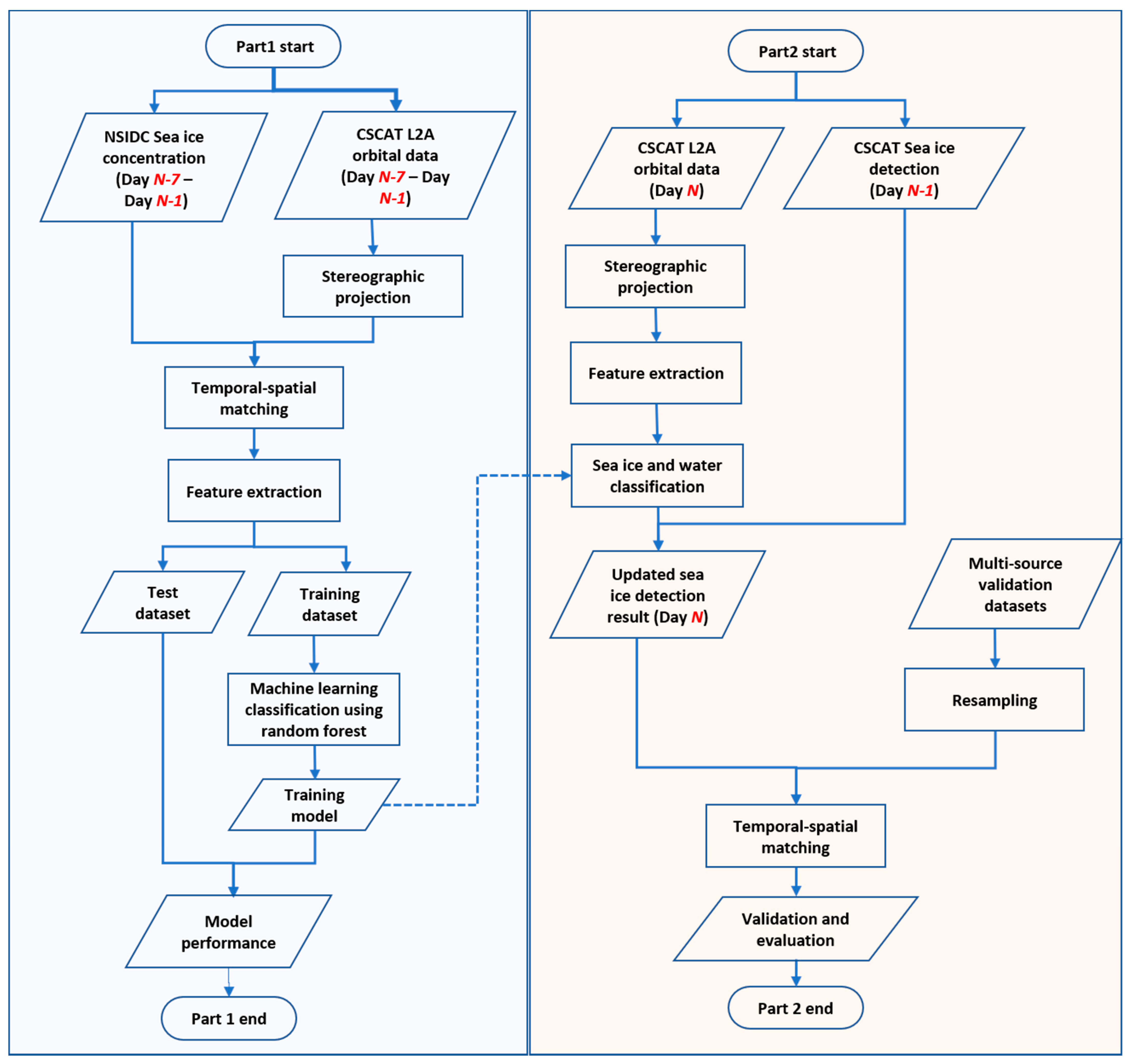
Figure 3 shows the flowchart of sea ice monitoring based on machine learning with CSCAT measurement in this study. Generally, the algorithm consists of two modules: the timing module (part 1, marked with blue rectangle area) and real-time module (part 2, marked with orange rectangle area).

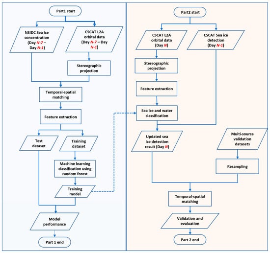
Figure 3. The flowchart of sea ice monitoring based on machine learning with CSCAT measurement.

The main process of the timing module is to train and evaluate the machine learning training model for sea ice monitoring. Taking sea ice variation from different seasons and years into consideration, in particular at the start and end of the melting and freezing seasons, the training model is updated based on the training dataset from the preceding 7 days. The reason the preceding 7-day datasets are used for model training will be specifically evaluated in Section 3.2. The input CSCAT ${\sigma }_0$ measurements (contained in Level 2A products) are resampled into polar ice maps with a pixel size of 25 km × 25 km using the polar stereographic projection firstly. Then the NSIDC sea ice concentration is matched for each pixel of the ice map. After the data preprocessing mentioned above, the feature parameters derived from the ${\sigma }_0$ measurement need to be computed to distinguish sea ice from water, which will be described in Section 3.1. To determine the optimal machine learning classification method for operational processing of sea ice monitoring, the several machine learning classification methods are assessed by a comprehensive evaluation in terms of the model accuracy, the difficulty of algorithm parameter optimization and debugging, the time efficiency, and other aspects of different classification methods. This process will be specifically described in Section 3.2. Finally, the trained training model deriving from the optimal machine learning algorithm will be used for the real-time module processing.

The input data of the real-time module includes the daily CSCAT ${\sigma }_0$ measurements and the sea ice monitoring result of the previous day. After the stereographic projection and feature extraction of ${\sigma }_0$ measurements, the automatic classification over the corresponding projected grid cells using the trained training model exported from the timing module are processed and updated. The uncertainty estimates of CSCAT sea ice monitoring are defined using the probability of predicted surface class, which indicates more details of the prediction accuracy in each grid cell. Finally, the inter-comparison is made between CSCAT sea ice results and validation datasets.

3.1. Extraction of Features

A difference in the scatterometer backscatter measurement exists due to the differences of the surface target in physical structure, dielectric permittivity, salinity, temperature, and other aspects. Generally, the radar backscattering amplitude over land or ice is stronger than over ocean, except for in high sea surface wind conditions. Specifically, the scatterometer measurement relies on surface Bragg scattering from wind-generated waves over the ocean, while the scattering of sea ice is a mixture of volume and surface scattering. It is noted that wind-induced surface roughness can result in ambiguous signatures. Furthermore, the incidence angle, azimuthal and temporal dependence of ${\sigma }_0$ measurement over the ocean is generally much stronger than that over the ice. In addition, the copolarization (copol) ratio, defined as the ratio of ${\sigma }_{vv}$ and ${\sigma }_{hh}$, is a useful parameter for discriminating sea ice and water, where the ${\sigma }_{vv}$ or ${\sigma }_{hh}$ is the ${\sigma }_0$ measurement at a given incidence angle. Another similar parameter, named the modified copol ratio, exhibits a combination of polarization and incidence angle dependences of ocean and sea ice. Both copol ratio and modified copol ratio have a similar signature in that sea ice has a lower ratio than that of ocean. Last but not least, since the surface of multi-year ice is rougher than that of first-year ice, the scatterometer measurement from multi-year ice should be stronger than the first-year ice, which can be used for sea ice type classification.

Many studies have combined the physical mechanisms mentioned above with the characteristics of different scatterometer viewing geometries to extract the features for sea ice monitoring. The feature extraction in previous studies was basically derived from averaged daily observational datasets [33]. Since CSCAT has the advantage of large sample observation, all features used in this study are based on every ${\sigma }_0$ data contained in L2A product, rather than one-day dataset. Specifically, five parameters are defined for sea ice monitoring in this study. The first and second parameters are the mean value of horizontal and vertical polarization backscatter, respectively, which are defined as,

$${\overline{\sigma }}_{hh}=\frac{1}{N}{\displaystyle \sum _{i=1}^N{\sigma }_{hh,i}({\theta }_i,{\varphi }_i)},$$

(1)

$${\overline{\sigma }}_{vv}=\frac{1}{N}{\displaystyle \sum _{i=1}^N{\sigma }_{vv,i}({\theta }_i,{\varphi }_i)}$$

(2)

where N is the number of observations at the grid cell after stereographic projection, ${\sigma }_{hh,i}({\theta }_i,{\varphi }_i)$ and ${\sigma }_{vv,i}({\theta }_i,{\varphi }_i)$ are the ith horizontal and vertical polarization backscatter, respectively, and ${\theta }_i$ and ${\varphi }_i$ are the corresponding incidence and azimuth angle, respectively.

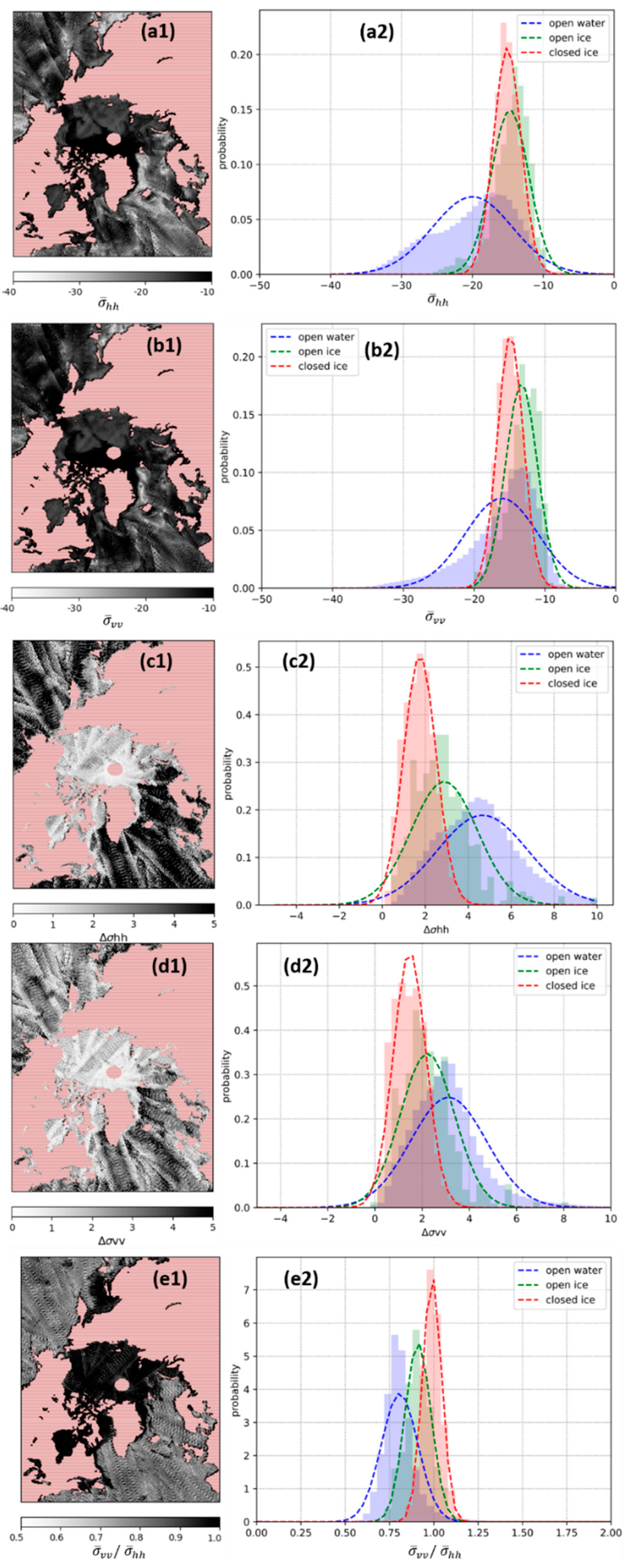
It can be seen that ${\overline{\sigma }}_{hh}$ and ${\overline{\sigma }}_{vv}$ mainly rely on different scattering mechanisms between sea ice and ocean. The difference from previous studies is that both the incidence and azimuth angles can affect these parameters’ performance to some extent. Figure 4(a1, b1) shows the example image of ${\overline{\sigma }}_{hh}$ and ${\overline{\sigma }}_{vv}$ on 8 April 2020. Compared with Figure 2, it is clear that both ${\overline{\sigma }}_{hh}$ and ${\overline{\sigma }}_{vv}$ are much lower in the ocean region than the sea ice region as expected. Furthermore, the difference between multi-year ice and first-year ice is quite significant, proving the feasibility of ${\overline{\sigma }}_{hh}$ and ${\overline{\sigma }}_{vv}$ for sea ice type distinguishment, which will be analyzed in a further study. Figure 4(a2,b2) shows the distribution of ${\overline{\sigma }}_{hh}$ and ${\overline{\sigma }}_{vv}$ for three ice edge classes, that is, open water, open ice, and closed ice, respectively, based on collocated data from 1 April 2020 to 7 April 2020 in the Arctic region. It is seen that a Gaussian approximation holds good for the open water class, but the distributions of open ice and closed ice are asymmetric. Furthermore, the statistical distribution of open water and ice (open ice + closed ice) is clearly distinguished, but that is not the case between open ice and closed ice.

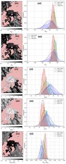
Figure 4. Parameters derived from one day of CSCAT measurements in the Arctic on 7 March 2019. (a1) ${\overline{\sigma }}_{hh}$, (b1) ${\overline{\sigma }}_{vv}$, (c1) $\Delta {\sigma }_{hh}$, (d1) $\Delta {\sigma }_{vv}$ and (e1) $\gamma$. Arctic images contain 448 × 304 pixels with a pixel resolution of 25 km. The central white circular area represents no observations. Density plot for parameters (a2) ${\overline{\sigma }}_{hh}$, (b2) ${\overline{\sigma }}_{vv}$, (c2) $\Delta {\sigma }_{hh}$, (d2) $\Delta {\sigma }_{vv}$, and (e2) $\gamma$ for open water (blue), open ice (green), and closed ice (red).

The third and fourth parameters are the standard deviations of horizontal and vertical polarization measurements respectively, which are defined as,

$$\Delta {\sigma }_{hh}=\sqrt{\frac{1}{N}{\displaystyle \sum _{i=1}^N{[{\sigma }_{hh,i}({\theta }_i,{\varphi }_i)-{\sigma }_{hh}]}^2}},$$

(3)

$$\Delta {\sigma }_{vv}=\sqrt{\frac{1}{N}{\displaystyle \sum _{i=1}^N{[{\sigma }_{vv,i}({\theta }_i,{\varphi }_i)-{\sigma }_{vv}]}^2}}$$

(4)

Similar to ${\overline{\sigma }}_{hh}$ and ${\overline{\sigma }}_{vv}$, $\Delta {\sigma }_{hh}$ and $\Delta {\sigma }_{vv}$ are affected by the incidence and azimuth angles simultaneously. $\Delta {\sigma }_{hh}$ and $\Delta {\sigma }_{vv}$ mainly rely on the difference of the incidence and azimuthal dependence of scatterometer measurements over sea ice and ocean. Figure 4(c1,d1) shows the example image of $\Delta {\sigma }_{hh}$ and $\Delta {\sigma }_{vv}$ on 8 April 2020. Compared with Figure 2, it is clear that both $\Delta {\sigma }_{hh}$ and $\Delta {\sigma }_{vv}$ are much lower in the sea ice region than the ocean region, coinciding with the fact that the incidence and azimuthal angle dependence of scatterometer measurement over ocean is much deeper. It is noted that $\Delta {\sigma }_{hh}$ and $\Delta {\sigma }_{vv}$ shown in Figure 4(c2,d2) has more obvious textures in the outer swath edge than ${\overline{\sigma }}_{hh}$ and ${\overline{\sigma }}_{vv}$ shown in Figure 4(a1,b1), where the corresponding values are generally lower than in the other swath regions. This is because the diversity of incidence angles and azimuth angles of measurements are much lower in the outer swath than other swath regions, as shown in Figure 1. Similar to Figure 4(a1,b1), Figure 4(c2,d2) shows the distribution of $\Delta {\sigma }_{hh}$ and $\Delta {\sigma }_{vv}$ for open water, open ice, and closed ice, respectively. It is seen that the statistical distribution of open water and closed ice for $\Delta {\sigma }_{hh}$ can be distinguished better than that of $\Delta {\sigma }_{vv}$ in this case.

The fifth parameter is the copol ratio $\gamma$, defined as the ratio of ${\overline{\sigma }}_{vv}$ and ${\overline{\sigma }}_{hh}$, i.e., $\gamma ={\overline{\sigma }}_{vv}/{\overline{\sigma }}_{hh}$. Figure 4(e1) shows the example image of $\gamma$ on 8 April 2020. It is shown that the $\gamma$ is much higher over sea ice than that over ocean. And $\gamma$ can eliminate the orbital edge effect very well. The Gaussian approximation shows good discrimination between open water and closed sea ice, and these three classes can be well fitted by a Gaussian model.

3.2. Machine Learning-Aided Sea Ice Monitoring Methods

In order to make comprehensive use of the above five feature parameters to distinguish sea ice distribution, five machine learning classifiers are evaluated firstly [43], including logistic regression, naïve Bayes, random fore gradient boosting, and support vector machine (SVM).

Specifically, the training and prediction speed of logistic regression is very fast which is suitable for very large datasets and high-dimensional data. However, the generalization performance of other models may be better in the lower dimensional space. Naive Bayes classifier learns parameters by looking at each feature individually, and collecting simple statistical data from each feature. It has a faster training speed, but its generalization ability is slightly worse than logistic regression classifier. Random forest and gradient boosting classifiers belong to the ensemble learning method, both of which are based on the decision tree method. The main disadvantage of the decision tree is overfitting. The strategery of the random forest classifier is to use a bootstrap sample when constructing decision tree and random feature subset at each node. The gradient boosting classifier constructs trees in a continuous way, and each tree tries to correct the error of the previous tree through continuously monitoring its own cumulative error and then using the residual for subsequent training. The SVM classifier transforms the input parameter vector into a high-dimensional space, and finds the optimal linear classification surface in this new high-dimensional space to solve the nonlinear problem.

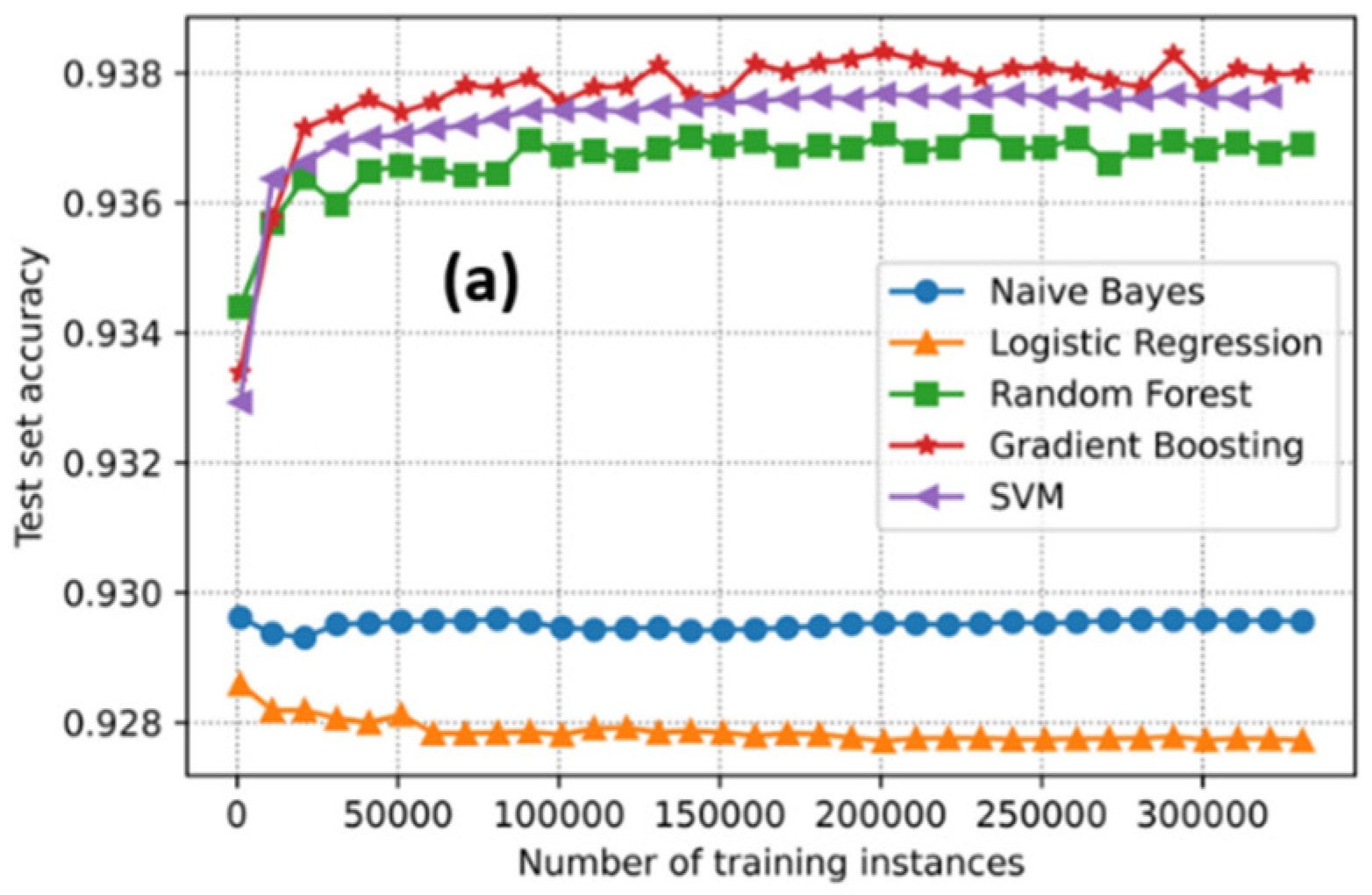
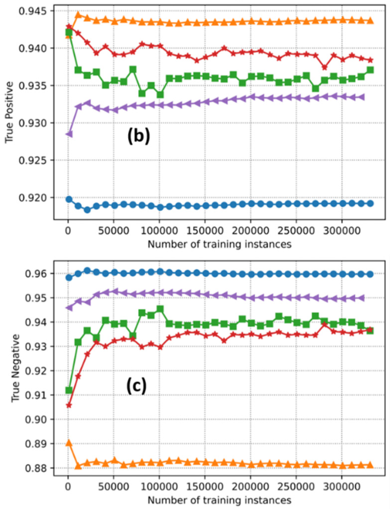
Taking the Arctic sea ice distribution model as an example, the NSIDC sea ice concentration is used as priori information to identify the sea ice and water in the CSCAT observation area. As shown in Figure 5, the five classifiers mentioned above are evaluated from three aspects, that is, the model accuracy derived from test dataset, the accuracy of water discrimination (true positive), and the accuracy of sea ice discrimination (true negative), respectively. It is noted that the parameters of each classifier have been optimized before evaluation. Ideally the time period of the training data should be as short as possible to best represent the actual ice condition, however the length is also determined by the need to collect enough training data to derive reliable statistics. The relationship between the training instances and these three aspects shows that when the number of training sets is more than 50,000, which is equivalent to a week’s dataset, the change of accuracy is not improved as a whole, indicating the reliability of using previous one-week data for model training. In addition, the model accuracies of SVM, gradient boosting and random forest are superior to logistic regression and Naive Bayes. Since the training of SVM is very time-consuming, and the gradient boosting requires more parameter adjustment process, the random forest classifier is selected for sea ice monitoring in this study. In this case, the accuracies of sea ice and water are 0.94, 0.98, respectively, and the importance of feature parameters is ranked as follows: ${\overline{\sigma }}_{hh}>\Delta {\sigma }_{hh}>\gamma >\Delta {\sigma }_{vv}>{\overline{\sigma }}_{vv}$.

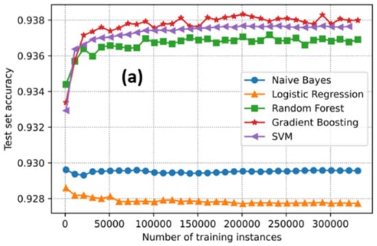
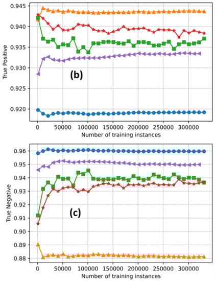
Figure 5. The performance evaluation of different training models: the relationship between the number of training instances and (a) the test set overall accuracy, (b) true positive rate (accuracy of sea water discrimination), and (c) true negative rate (accuracy of sea ice discrimination). The blue, orange, green, red, and purple marked-lines represent the results from Naive Bayes, logistic regression, random fore gradient boosting, and support vector machine (SVM) classification, respectively.

4. Results

The model performance and retrieval results from 1 January 2019 to 10 May 2021 are analyzed in this section. However, because of quality control, there are 56 days and 110 days in the Arctic and Antarctic that were skipped respectively firstly, and the specific corresponding dates and reasons for elimination are shown in Table 5. The number of days used for statistical analysis in the Arctic and Antarctic accounted for 93.5% and 87.3%, respectively, ensuring the representativeness of the further evaluation.

Table 5. The list of invalid dates and reason for statistical analysis from 1 January 2019 to 10 May 2021.

Data Source	Invalid Date In Arctic	Invalid Date In Antarctic	Invalid Reason (Removed Quantity)
CSCAT	4 January 2019 17 April 2019 18 May 2019 30 May–5 June 2019 19 June 2019 2 July 2019 17 July 2019 28 August 2019 1 October 2019 2–7 February 2020 14 April 2020 15 June 2020 27 June 2020 9 July 2020 29–30 December 2020 9 January 2021 31 January 2021 24 February–4 March 2021	4 January 2019 17 April 2019 18 May 2019 30 May–5 June 2019 19 June 2019 2 July 2019 17 July 2019 28 August 2019 1 October 2019 2–7 February 2020 14 April 2020 15 June 2020 27 June 2020 9 July 2020 3 August–1 September 2020 15 November–10 December 2020 29–30 December 2020 9 January 2021 31 January 2021 20 February–4 March 2021	Quality control elimination (Arctic: 38 Antarctic: 92)
CSCAT	19 December 2019–14 January 2020 29 December 2020		No data
NSIDC sea ice concentration	20–23 February 2021		No data

4.1. Characteristics of CSCAT Feature Parameters

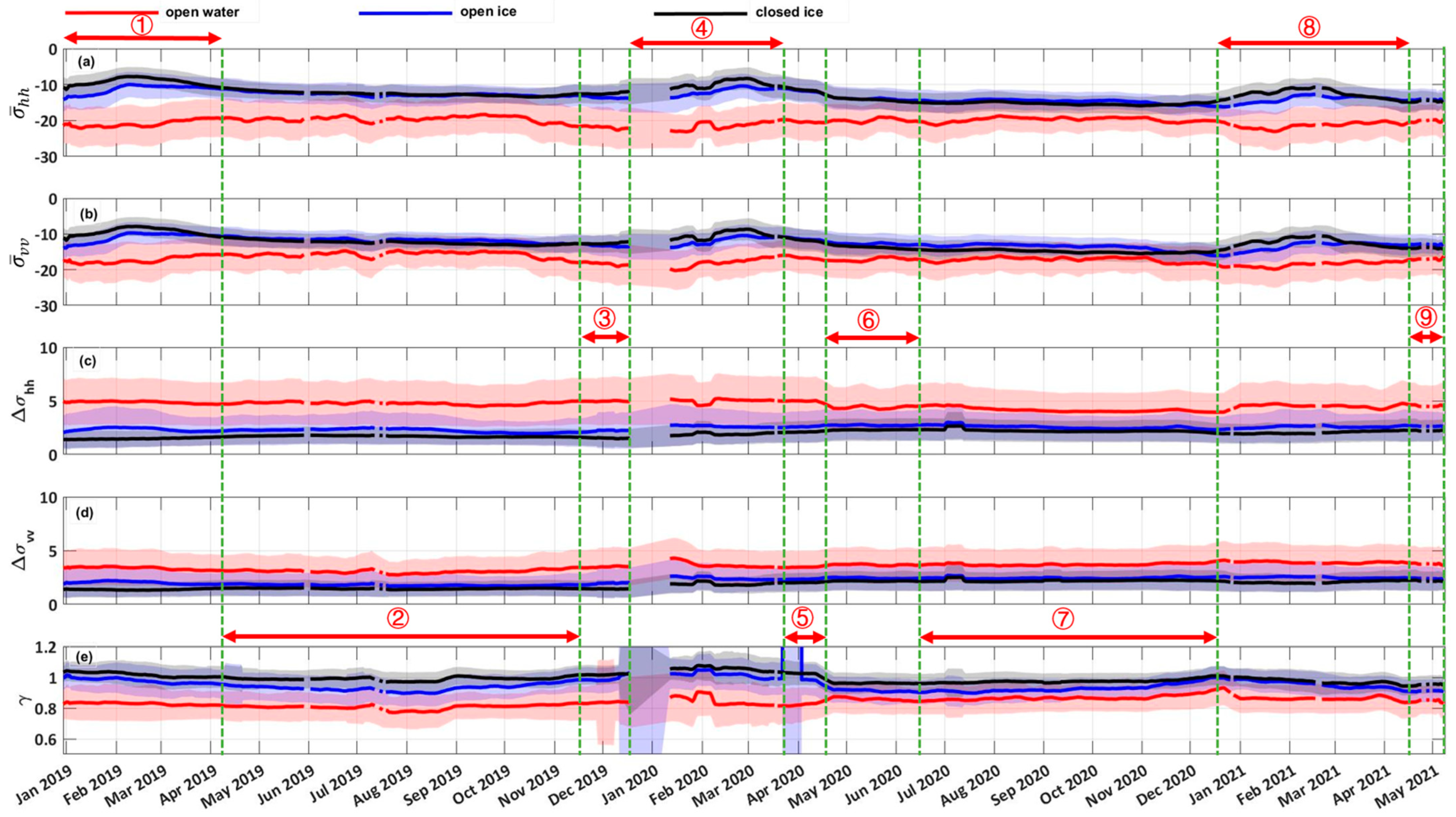
Figure 6 shows the PDF’s mean values and standard deviations of sea ice distribution feature parameters from 1 January 2019 to 10 May 2021 in the Arctic. It is noted that when the standard deviation-regions of the different classes are distinctively different, the algorithm should do well in the classification, whereas overlapping between the different PDF’s causes uncertainties in the classification.

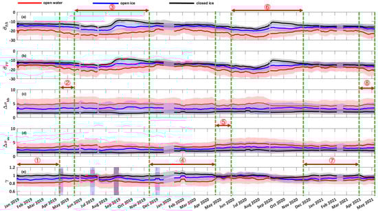
Figure 6. The mean values (solid lines) and standard deviations (shaded areas) of Arctic sea ice distribution feature parameters from 1 January 2019 through 10 May 2021 (a) ${\overline{\sigma }}_{hh}$, (b) ${\overline{\sigma }}_{vv}$, (c) $\Delta {\sigma }_{hh}$, (d) $\Delta {\sigma }_{vv}$, (e) $\gamma$. The red, blue, and black marked results represent open water, open ice, and closed ice, respectively. The double arrows represent the most significant feature parameters in different time periods.

In Figure 6a,b, the time series of ${\overline{\sigma }}_{hh}$ and ${\overline{\sigma }}_{vv}$ show distinctly seasonal trends. During summer, the moisture at the surface produces lower backscatter due to a scattering mechanism change from volume scattering to surface scattering. While during winter, the refreezing process results in stronger backscatter, which is consistent with previous studies. $\Delta {\sigma }_{hh}$, $\Delta {\sigma }_{vv}$ and $\gamma$ don’t change significantly with the seasons, as shown in Figure 6c–e. According to the difference of the most significant feature parameters in the training model, it is divided into eight periods (represented by double arrows) in the Arctic. Specifically, $\gamma$ dominates the training model at the end of autumn and the whole winter time, and the $\Delta {\sigma }_{hh}$ or $\Delta {\sigma }_{vv}$ has a significant effect at the end of winter and the beginning of spring, while in the spring, summer and autumn periods, ${\overline{\sigma }}_{hh}$ performs best for sea ice prediction.

Similarly, Figure 6 and Figure 7 show the statistical results of ${\overline{\sigma }}_{hh}$, ${\overline{\sigma }}_{vv}$, $\Delta {\sigma }_{hh}$, $\Delta {\sigma }_{vv}$ and $\gamma$ in Antarctic. As shown in Figure 7a,b, the time series of ${\overline{\sigma }}_{hh}$ and ${\overline{\sigma }}_{vv}$ in the Antarctic also have distinct seasonal trends, and the difference between water and ice is more distinct than that in the Arctic, but the difficulty lies in the distinguishment between open ice and closed ice, which is almost indistinguishable except for in the summer period. $\Delta {\sigma }_{vv}$, ${\sigma }_{vv}$ and $\gamma$ don’t change significantly with the seasons in the Antarctic either, as shown in Figure 7c–e. Nine periods are divided based on the difference of the most significant feature choice. Specifically, ${\overline{\sigma }}_{hh}$ dominants the training model in summer, and the $\gamma$ has a significant effect in spring, autumn, and winter periods, while at the end of spring and the beginning of summer, or at the end of autumn and beginning of winter, $\Delta {\sigma }_{hh}$ performs best for sea ice prediction. The difference in feature important rank in the different seasons implies that the combination of these parameters is effective in discriminating sea ice from water under various conditions.

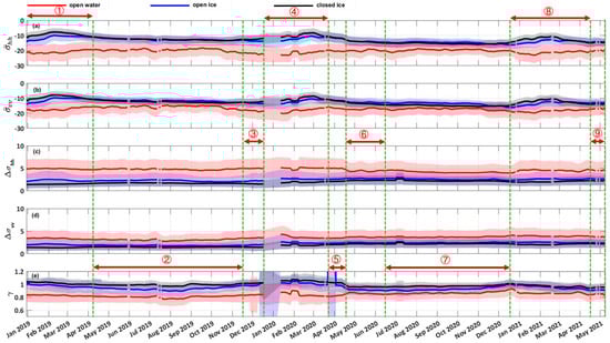
Figure 7. The mean values (solid lines) and standard deviations (shaded areas) of Antarctic sea ice distribution feature parameters from 1 January 2019 through 10 May 2021 (a) ${\overline{\sigma }}_{hh}$, (b) ${\overline{\sigma }}_{vv}$, (c) $\Delta {\sigma }_{hh}$, (d) $\Delta {\sigma }_{vv}$, (e) $\gamma$. The red, blue, and black marked results represent open water, open ice, and closed ice, respectively. The double arrows represent the most significant feature parameters in different time periods.

4.2. Evaluation of Sea Ice Distribution Model Precision

The sea ice monitoring models based on random forest classifier are quantitatively assessed using a confusion matrix through a comparison with the NSIDC sea ice concentration data as reference data. Each column of the confusion matrix represents the prediction category, and the total number of each column represents the number of data predicted as the category. Similarly, each row represents the real category of data, and the total amount of data in each row represents the number of data instances in that category. The overall accuracy, kappa coefficient, and the precision, recall, and F1 measurement for specific categories are derived from the confusion matrix. Specifically, the accuracy and kappa coefficient are used to evaluate the overall prediction accuracy of the model. The precision per category is defined as the ratio of all samples with correct prediction to the total samples in this prediction category. The recall per category represents the proportion of samples correctly predicted in a real category. The F1 measurement is used as a comprehensive index to take both precision and recall into account.

It should be noted that in the multi-classification model, each type needs to calculate its precision and recall separately, so the true positive (TP), true negative (TN), false positive (FP), and false negative (FN) defined for different types are different. Taking open water as an example, $T{P}_{openwater}$ is defined as the number of actual open water and predicted open water, and $T{N}_{openwater}$ is defined as the number of actual sea ice (open ice or closed ice) and predicted sea ice. $F{P}_{openwater}$ is defined as the number of actual sea ice but predicted open water, and $F{N}_{openwater}$ is defined as the number of actual open water but predicted sea ice. Therefore, the precision and recall of open water are defined as:

$$Precisio{n}_{openwater}=\frac{T{P}_{openwater}}{T{P}_{openwater}+F{P}_{openwater}},$$

(5)

$$Recal{l}_{openwater}=\frac{T{P}_{openwater}}{T{P}_{openwater}+F{N}_{openwater}},$$

(6)

Figure 8 and Figure 9 show the time series of the parameters described above to evaluate sea ice monitoring training models in the Arctic and Antarctic from January 1 2019 through May 10 2021, respectively, the averaged classification accuracies of which are summarized in Table 6. Before specific analysis, it should be noted that as for supervised classification learning which is used in this study, the collected labeled dataset is generally divided into two parts: training set and test set, to evaluate the accuracy of the training model. It should be emphasized that these two parts of data are independent of each other. Specifically, the training set is used to build the model, and the test set is used to evaluate the generalization ability of the model to new data that has never been seen before. In this paper, NSIDC sea ice concentration is used to define the label of ice water classification. Part of the data (called training set) is used to build the ice water discrimination model, and the rest of the data (called test set) is used to evaluate the model performance. The two are not contradictory, and the results of Table 6 further illustrate the good generalization ability of the training model to new data.

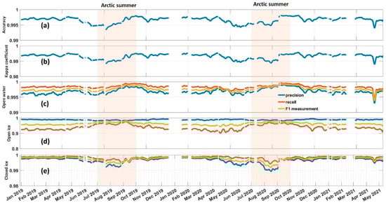
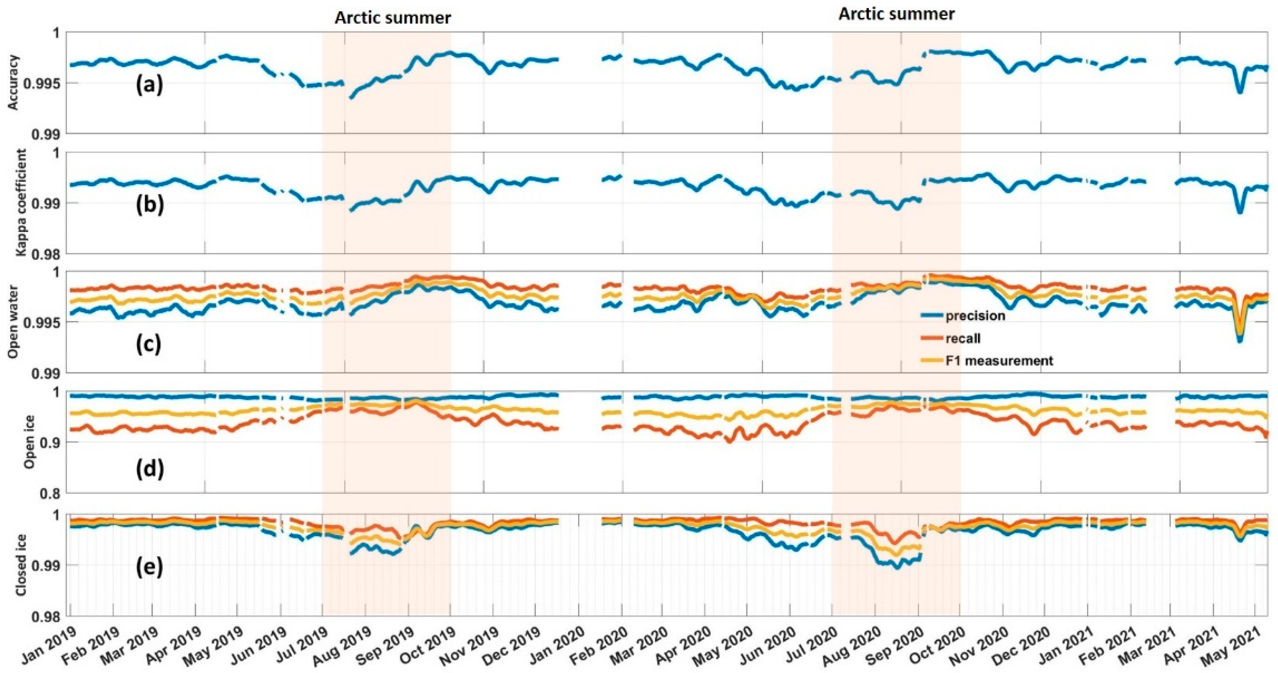
Figure 8. The time series of the evaluation parameters of the sea ice monitoring training model in the Arctic from 1 January 2019 through 10 May 2021 for (a) the overall accuracy, (b) kappa coefficient, (c) open water, (d) open ice, and (e) closed ice, respectively.

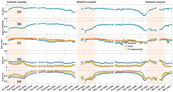
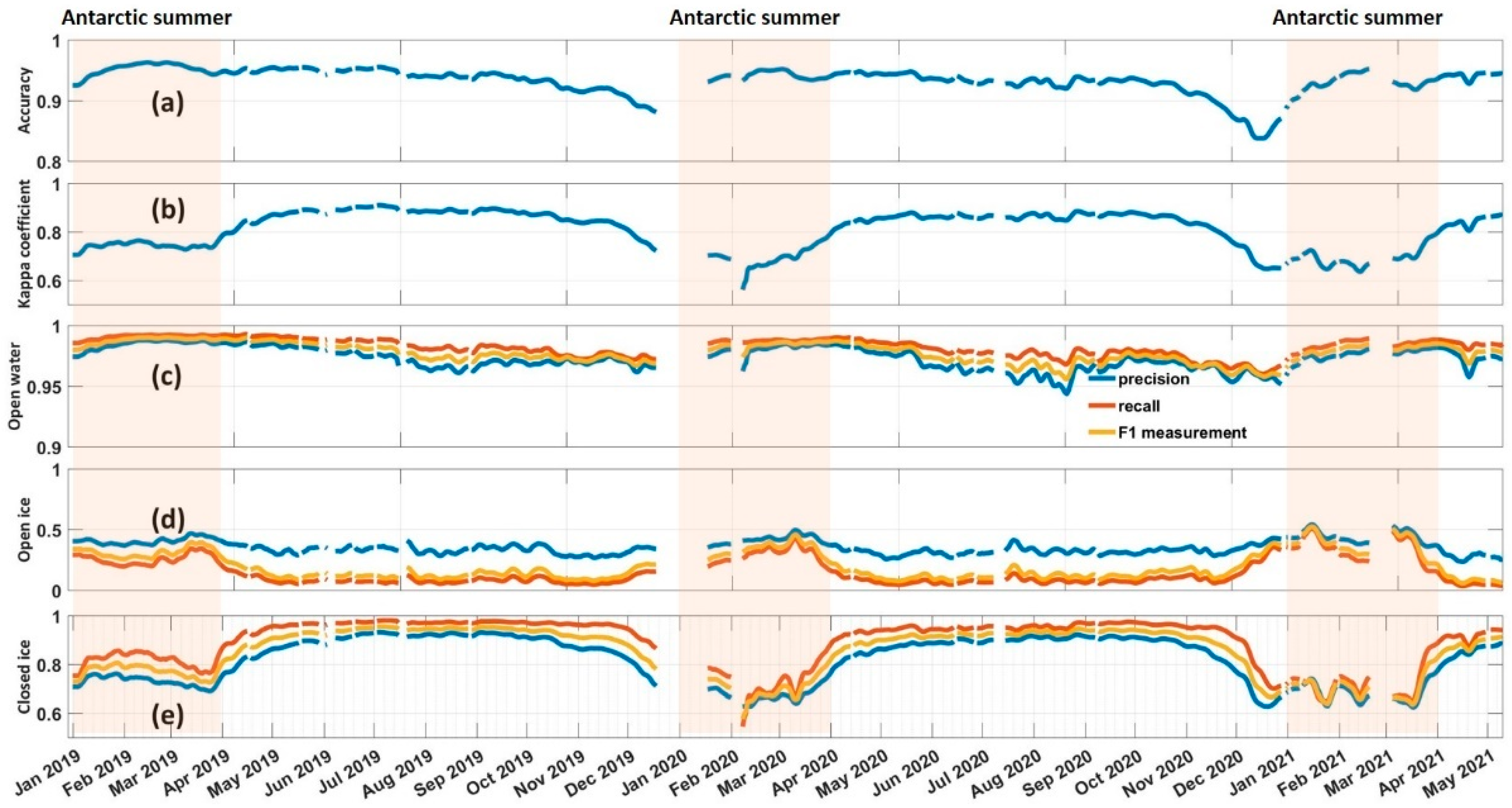
Figure 9. The time series of the evaluation parameters of the sea ice monitoring training model in the Antarctic from 1 January 2019 through 10 May 2021 for (a) the overall accuracy, (b) kappa coefficient, (c) open water, (d) open ice, and (e) closed ice, respectively.

Table 6. Summary of averaged classification accuracies obtained through a random forest classifier in the Arctic and Antarctic from 1 January 2019 through 10 May 2021.

Region	Classification	Precision	Recall	F1 Measurement	Overall Accuracy	Kappa Coefficient
Arctic	Open water	99.69%	99.84%	99.76%	99.66%	99.31%
	Open ice	98.77%	93.80%	96.21%
	Closed ice	99.65%	99.82%	99.74%
Antarctic	Open water	97.29%	98.23%	97.75%	93.31%	80.77%
	Open ice	35.29%	14.95%	19.70%
	Closed ice	81.8%	88.9%	85.15%

The overall accuracy and kappa coefficient for the Arctic are quite high: 99.66%, 99.31% on average, respectively. The precision, recall, and F1 measurement of open water and closed ice are obviously higher than those of open ice. As shown in Figure 10, the reasons for lower accuracies of open ice are slightly different in different seasons. Specifically, at the end of the summer and the whole autumn season, the open ice is easily misclassified as open water, while the open ice is easier to be misjudged as closed ice at the end of winter and the whole spring season.

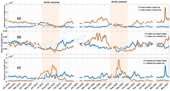
Figure 10. The error analysis of the Arctic sea ice monitoring training models from 1 January 2019 through 10 May 2021: (a) open water is misclassified as open ice (blue line) and closed ice (red line), respectively, (b) open ice is misclassified as open water (blue line) and closed ice (red line), respectively, and (c) closed ice is misclassified as open water (blue line) and open ice (red line), respectively.

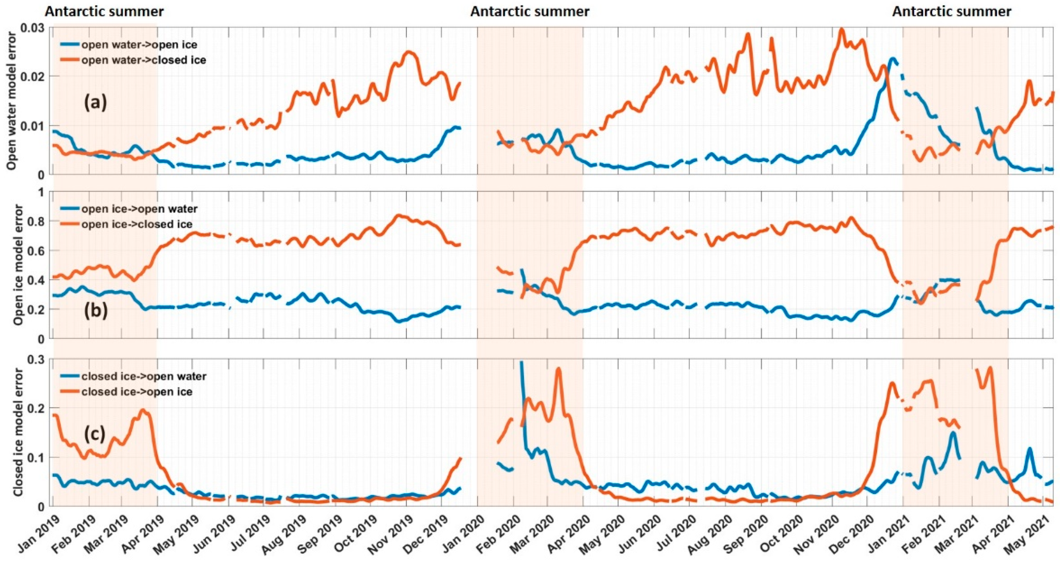
The overall accuracy and kappa coefficients for the Antarctic are 93.31% and 80.77% on average, respectively, which are much lower than the Arctic results. Furthermore, the kappa coefficient in the Antarctic is lower than 0.8 in summer, which is obviously lower than other seasons, indicating that the accuracy of the ice water identification model in the Antarctic is lower in summer. Similar to the evaluation result in the Arctic, the category most difficult to be classified is open ice, the precision, recall, and F1 measurement of which are 35.29%, 14.95%, and 19.70%, respectively. As shown in Figure 11b, the main reason for lower open ice accuracy in the Antarctic is the misclassification between open ice and closed ice. In addition, the accuracy of closed ice in the Antarctic also has seasonal variation, where lower accuracies appear in summer and the closed ice is easier to misclassify as open ice in the summer period.

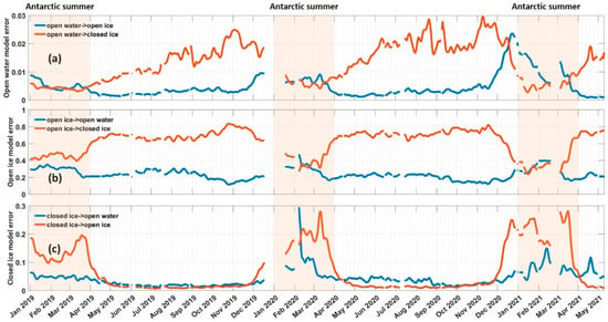
Figure 11. The error analysis of the Antarctic sea ice monitoring training models from 1 January 2019 through 10 May 2021: (a) open water is misclassified as open ice (blue line) and closed ice (red line), respectively, (b) open ice is misclassified as open water (blue line) and closed ice (red line), respectively, and (c) closed ice is misclassified as open water (blue line) and open ice (red line), respectively.

5. Discussion

5.1. Daily Sea Ice Area Comparison with Different Datasets

In this study, sea ice area is computed as the sum of open ice and closed ice area, and assuming the areas not covered by CSCAT in center of the North Pole (as shown in Figure 4) are entirely covered by sea ice. Figure 12a shows the comparison of sea ice area obtained from different data sources in the Arctic, where blue, red and yellow lines represent the results of CSCAT, NSIDC ice 40% extent, and OSI SAF sea ice edge product, respectively. An excellent consistency in the seasonal variation among all three results can be seen in Figure 12a. In order to quantitatively compare the difference in sea ice area, the sea ice area relative error $R{E}_{ice}$ and difference $\Delta S_{ice}$ are defined as:

$$R{E}_{ice}=\frac{\Delta S_{ice}}{S_{reference,ice}}\times 100\%,$$

(7)

$$\Delta S_{ice}=S_{observation,ice}-S_{reference,ice}$$

(8)

where $S_{observation,ice}$ and $S_{reference,ice}$ refer to observational and reference results, respectively. $R{E}_{ice}$ represents the relative deviation percentage of the observational result compared with the reference one.

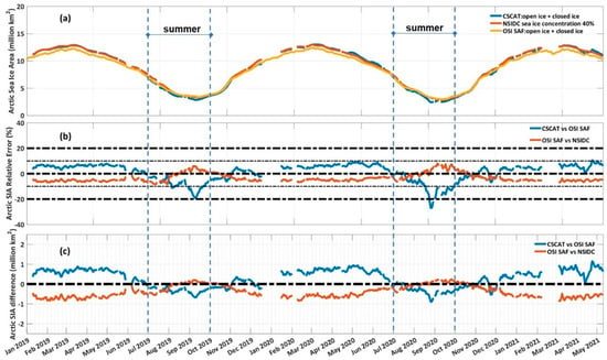
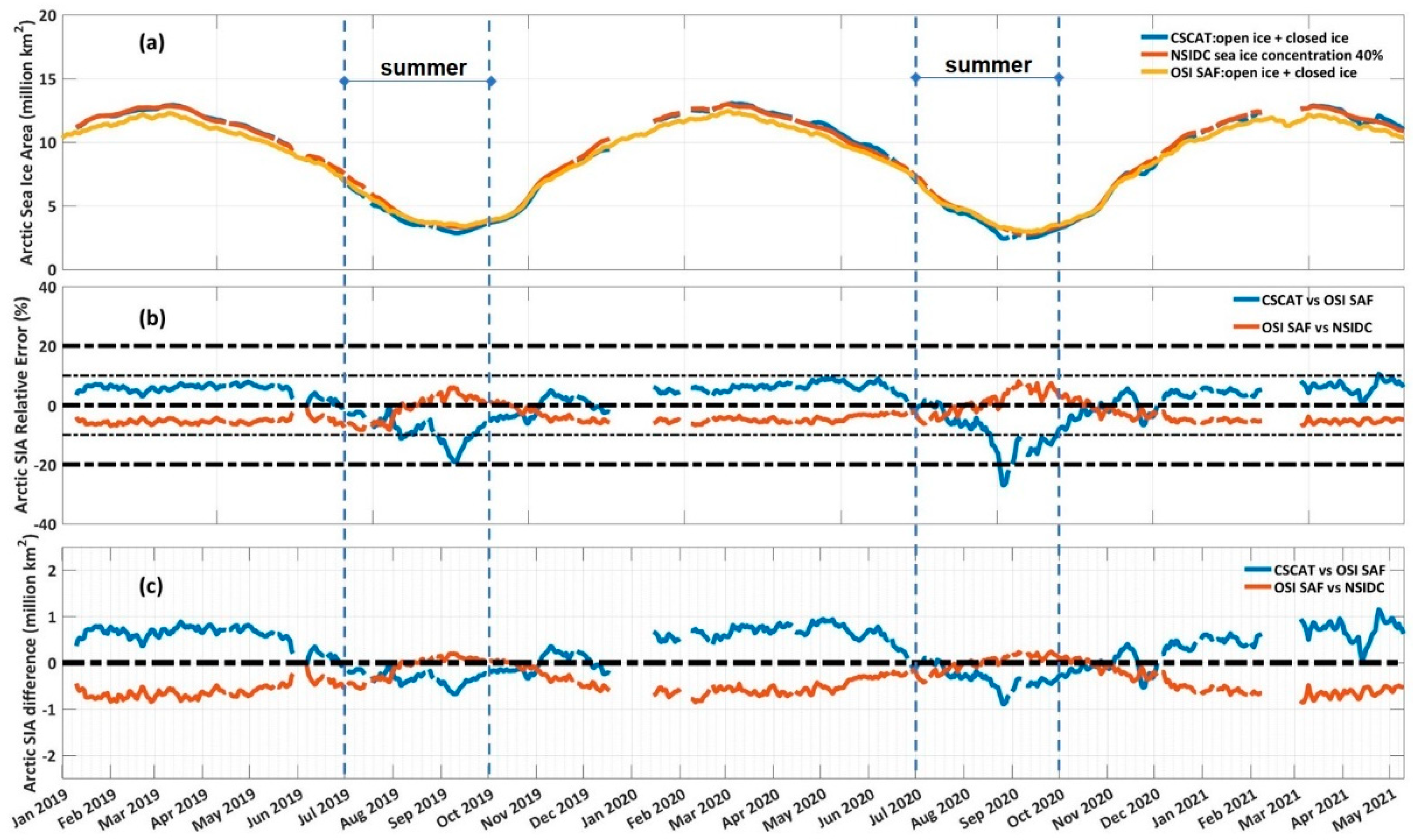
Figure 12. The Arctic results from 1 January 2019 through 10 May 2021 (a) daily sea ice area for CSCAT (blue line), NSIDC 40% ice extent (red line) and OSI SAF sea ice edge product (yellow line), respectively, (b) sea ice area relative error and (c) sea ice area difference between CSCAT and OSI SAF sea ice edge product (blue line), between OSI SAF sea ice edge product and NSIDC 40% ice extent (red line), respectively.

The comparison between CSCAT and OSI SAF in Arctic is shown in Figure 12b,c with blue lines. It can be seen that when the OSI SAF sea ice area is chosen as reference data, the absolute $R{E}_{ice}$ of CSCAT results are less than 20% in 99.2% of the time series, the corresponding $R{E}_{ice}$ mean value of which is 1.21%, and the absolute $R{E}_{ice}$ of CSCAT results are less than 10% with $R{E}_{ice}$ mean value of 2.45% in about 92.1% of the time series. In this case, the mean values of $\Delta S_{ice}$ between CSCAT and OSI SAF results is 0.2673 million km², implying that the sea ice area derived from CSCAT is a little bit larger than that of the OSI SAF results.

The comparison of the sea ice area between OSI SAF and NSIDC 40% ice extent in the Arctic is also evaluated and shown in Figure 12b,c with red lines. It can be seen that when NSIDC 40% ice extent is regarded as reference data, the absolute $R{E}_{ice}$ of OSI SAF results are less than 20% in whole time series with an $R{E}_{ice}$ mean value of −3.38%, and the absolute $R{E}_{ice}$ of OSI SAF results are less than 10% with $R{E}_{ice}$ mean value of −3.38% in whole time series. The mean values of $\Delta S_{ice}$ between OSI SAF and NSIDC 40% ice extent is −0.3873 million km², implying that the sea ice area derived from OSI SAF is less than that by NSIDC 40% ice extent results.

As shown in Figure 12, although different products perform well in overall consistency, obvious seasonal differences exist, especially in the summer period. Many studies [13,15,23,31,44] have shown that during sea ice melt and freeze-up phases, the radiation and backscatter properties of sea ice could change significantly, and the active and passive microwave sensors have a different sensitivity to the sea ice with mixed volume and surface scattering signatures. For instance, the passive microwave algorithms such as AMSR-E (or SSM/I) NT2 underestimate the extent of summer sea ice by up to 15%–20% relative to QuikSCAT [15]. In this study, CSCAT results are significantly underestimated compared with the OSI SAF sea ice area. The main reason is that the CSCAT is trained by radiometer sea ice concentration data while the radiometer measurement of sea ice is significantly affected by melting in the summer seasons [44], resulting in a larger discrepancy between CSCAT and OSI SAF sea ice results (noting that both scatterometer and radiometer data are used in OSI SAF sea ice edge product).

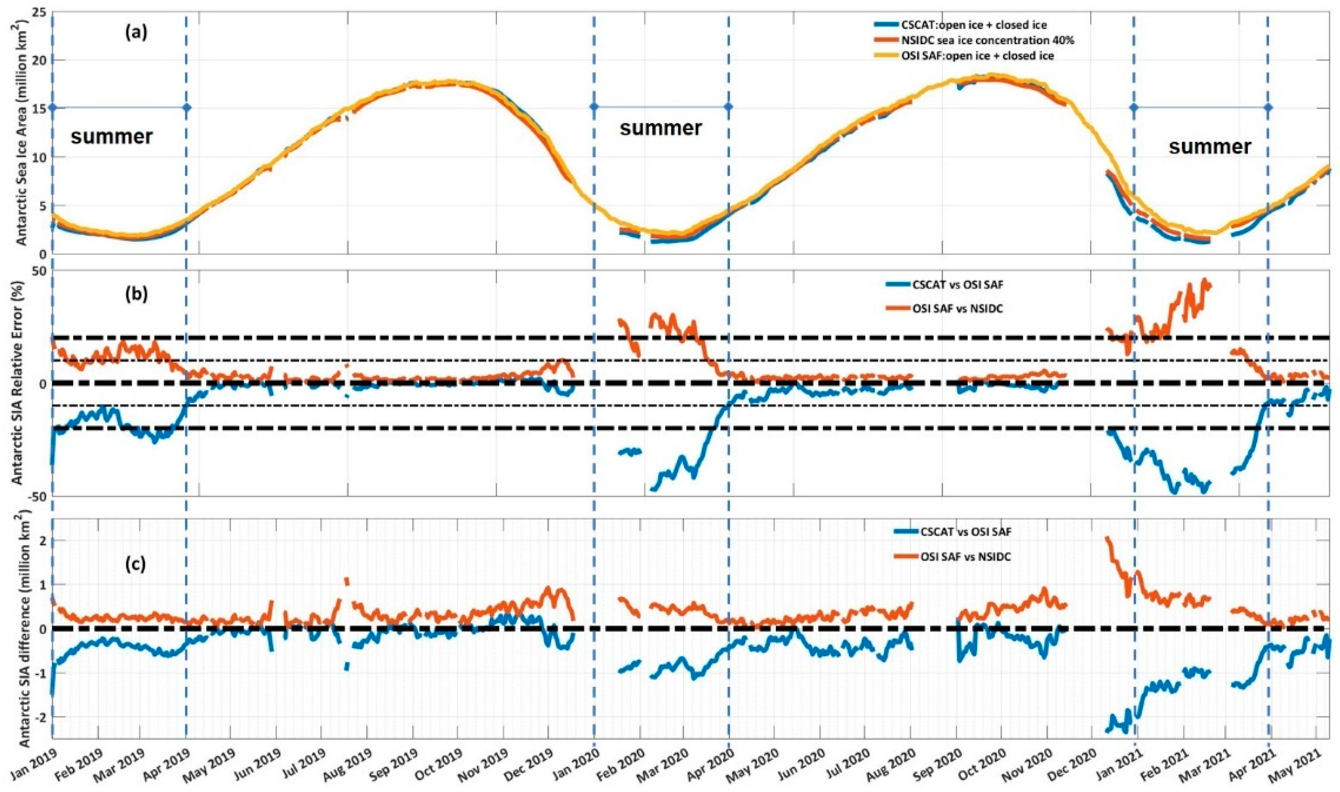
Figure 13 shows the time series statistics of the comparisons between CSCAT, OSI SAF, and NSIDC sea ice area in the Antarctic. Using similar analysis as Figure 12, it can be seen that when OSI SAF sea ice area is chosen as reference data, the absolute $R{E}_{ice}$ of CSCAT results are less than 20% in 79.2% of the time series, the corresponding $R{E}_{ice}$ mean value of which is −3.92%, and the absolute $R{E}_{ice}$ of CSCAT results are less than 10% with mean value of −2.18% in about 70.9% of the time series. In this case, the mean values of $\Delta S_{ice}$ between CSCAT and OSI SAF results is −0.4446 million km².

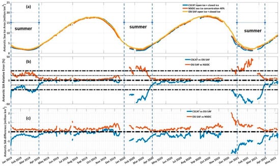
Figure 13. The Antarctic results from 1 January 2019 through 10 May 2021 (a) daily sea ice area for CSCAT (blue line), NSIDC 40% ice extent (red line), and OSI SAF sea ice edge product (yellow line), respectively, (b) sea ice area relative error, and (c) sea ice area difference between CSCAT and OSI SAF sea ice edge product (blue line), between OSI SAF sea ice edge product and NSIDC 40% ice extent (red line), respectively.

When NSIDC 40% ice extent is regarded as the reference data, the absolute $R{E}_{ice}$ of OSI SAF results are less than 20% in 89.6% of analyzed time series with an $R{E}_{ice}$ mean value of 5.04%, and the absolute $R{E}_{ice}$ of OSI SAF results are less than 10% with an $R{E}_{ice}$ mean value of 3.25% in about 78.1% of the time series. The mean values of $\Delta S_{ice}$ between OSI SAF and NSIDC 40% ice extent is 0.3736 million km². Similar to the results shown in Figure 12, both comparisons between these results in the Antarctic show significant seasonal fluctuations, where large discrepancies appear in the summer months of January–March.

Table 7 gives a summary of the comparison results described above. For both the Arctic and Antarctic area, when the OSI SAF sea ice area is regarded as reference data, the absolute $R{E}_{ice}$ of CSCAT are less than 10% except for in the summer season, verifying the reliability and stability of the algorithm. Furthermore, the overall sea ice area derived from CSCAT is lower than the OSI SAF sea ice area in the summer period. On the one hand, the model evaluation as shown in Figure 10b and Figure 11b implies that CSCAT open ice is easier to be misclassified as open water in the summer period. On the other hand, it may be the melt pond existence, where the active microwave feature parameters of sea ice are similar to sea water.

Table 7. Statistics of the comparisons between CSCAT, OSI SAF, and NSIDC sea ice area.

Region	${\mathit{S}}_{\mathit{o}\mathit{b}\mathit{s}\mathit{e}\mathit{r}\mathit{v}\mathit{a}\mathit{t}\mathit{i}\mathit{o}\mathit{n},\mathit{i}\mathit{c}\mathit{e}}$	${\mathit{S}}_{\mathit{r}\mathit{e}\mathit{f}\mathit{e}\mathit{r}\mathit{e}\mathit{n}\mathit{c}\mathit{e},\mathit{i}\mathit{c}\mathit{e}}$	$\mathbf{Proportion} \mathbf{of} \mathit{R}{\mathit{E}}_{\mathit{i}\mathit{c}\mathit{e},\left|20\mathit{\%}\right|}$ (%)	Mean Value of $\mathit{R}{\mathit{E}}_{\mathit{i}\mathit{c}\mathit{e},\left|20\mathit{\%}\right|}$ (%)	$\mathbf{Proportion} \mathbf{of} \mathit{R}{\mathit{E}}_{\mathit{i}\mathit{c}\mathit{e},|10\mathit{\%}|}$ (%)	$\mathbf{Mean} \mathbf{Value} \mathbf{of} \mathit{R}{\mathit{E}}_{\mathit{i}\mathit{c}\mathit{e},|10\mathit{\%}|}$ (%)	$\mathbf{Mean} \mathbf{Value} \mathbf{of} \Delta {\mathit{S}}_{\mathit{i}\mathit{c}\mathit{e}}$ (million km2)	$\mathbf{Standard} \mathbf{Deviation} \mathbf{of} \Delta {\mathit{S}}_{\mathit{i}\mathit{c}\mathit{e}}$ (million km2)
Arctic	CSCAT	OSI SAF	99.2	1.21	92.1	2.45	0.2673	0.4580
	OSI SAF	NSIDC	100	−3.38	100	−3.38	−0.3873	0.2958
Antarctic	CSCAT	OSI SAF	79.2	−3.92	70.9	−2.18	−0.4446	0.4895
	OSI SAF	NSIDC	89.6	5.04	78.1	3.25	0.3736	0.2653

5.2. Seasonal Sea Ice Area Comparison with Different Datasets

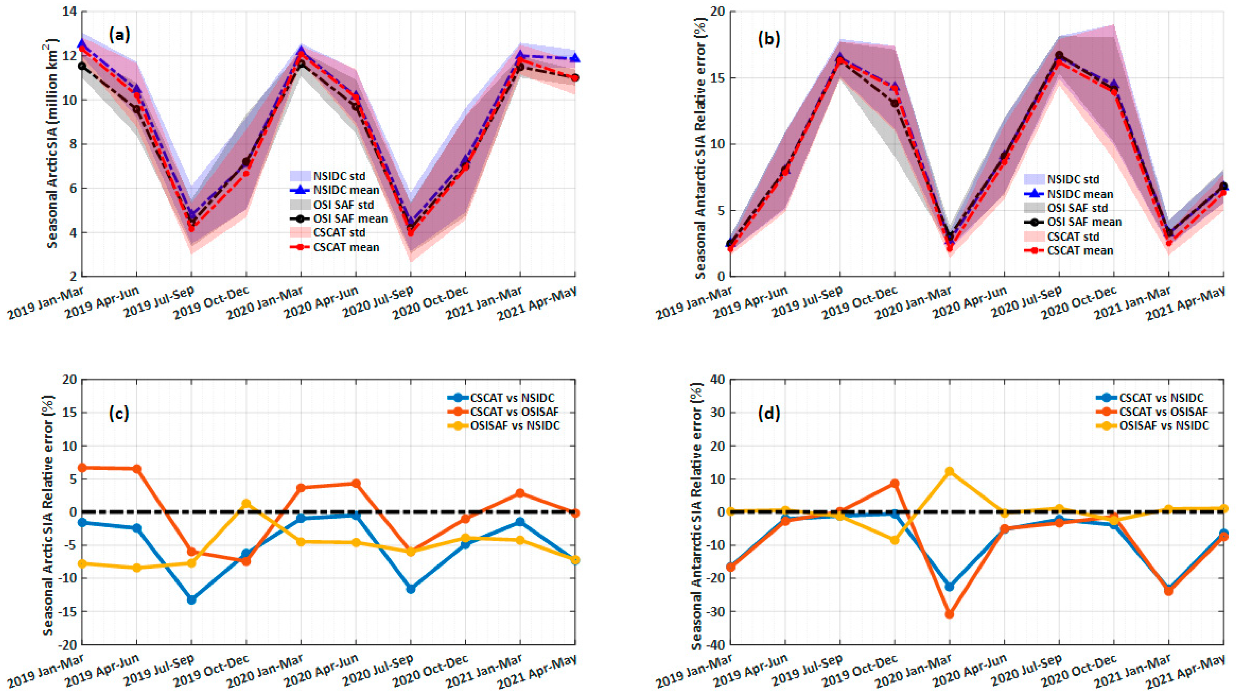
Figure 14a,b shows the seasonal variation trend of the Arctic and Antarctic sea ice area from different data sources. The red, blue, and black-marked results are derived from CSCAT, NSIDC 40% ice extent, and OSI SAF sea ice edge product, and the solid line and shadow represent the mean and standard deviation of sea ice area in corresponding seasons, respectively. The results show that the three types of results have good consistency in the seasonal variation of sea ice area. In the analyzed period, the minimum Arctic sea ice area of these three results all appear in July–September of 2020. However, the maximum Arctic sea ice area of NSIDC and CSCAT appears in January–March of 2019 with a mean value of 12.5112 million km² and 12.3123 million km², respectively, while the maximum Arctic sea ice area from OSI SAF appears in January–March of 2020 with a mean value of 11.6462 million km².

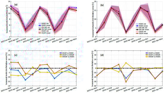
Figure 14. The mean values (dotted lines) and standard deviations (shaded areas) of seasonal sea ice areas from 1 January 2019 through 10 May 2021 for (a) the Arctic and (b) the Antarctic, respectively, where the blue, black, and red marked results represent NSIDC, OSI SAF, and CSCAT results, respectively. The seasonal sea ice area relative error for (c) the Arctic and (d) the Antarctic, respectively, where the blue, red, and yellow circled lines represent the comparison between CSCAT and NSIDC 40% SIC ice extent, between CSCAT and OSI SAF sea ice edge product, between OSI SAF sea ice edge product, and NSIDC 40% SIC ice extent, respectively.

As for Antarctic, the minimum Antarctic sea ice area of these three results all appears in January–March of 2019, while the maximum Antarctic sea ice area from NSIDC and OSI SAF appears in July–September of 2020 with a mean value of 16.5441 million km² and 16.7289 million km², respectively. The maximum Antarctic sea ice area from CSCAT appears in July–September of 2019 with a mean value of 16.3305 million km².

Figure 14c,d shows the relative error of the seasonal average of the Arctic and Antarctic sea ice areas. Consistent with the diurnal variation trend of Figure 12b and Figure 13b, the accuracy of CSCAT sea ice area fluctuates seasonally, and the CSCAT results are significantly underestimated compared with the OSI SAF sea ice area both in the Arctic and the Antarctic. The accuracy of the Arctic sea ice area is slightly higher than that of the Antarctic, which is related to the overall higher accuracy of the Arctic sea ice distribution training model than that of Antarctic training model.

5.3. CSCAT Sea Ice Edge Comparison with NSIDC SIC Datasets

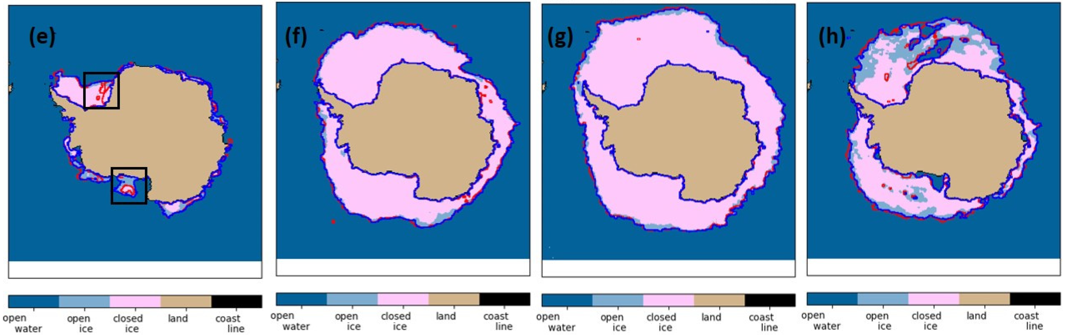
Figure 15a–h illustrate the seasonal and geographical behavior of the CSCAT and NSIDC (40% concentration threshold) sea ice masks for a limited subset of days in Arctic and Antarctic, respectively. It is noted that the residual classification errors of CSCAT are reduced using image erosion/dilation techniques and sea ice growth/retreat constraint methods. The agreement between the sea ice edges derived from CSCAT and NSIDC 40% ice extent is very good except for in the summer period. In this case, the discrepancy between CSCAT and NSIDC 40% ice extent for 7 September 2019 in the Arctic is due to the CSCAT misclassification of closed ice as open water, as shown in Figure 15c with a black rectangle-marked area. And the main difference between CSCAT and NSIDC 40% ice extent for 7 March 2019 in the Antarctic is mainly due to the CSCAT misclassification of open ice as open water, as shown in Figure 15e with a black rectangle-marked area.

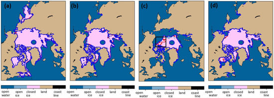
Figure 15. Comparison of sea ice edge from CSCAT retrieved result (red line) and NSIDC 40% SIC isoline (blue line): (a) the Arctic on 7 March 2019, (b) the Arctic on 7 June 2019, (c) the Arctic on 7 September 2019, (d) the Arctic on 7 December 2019, (e) the Antarctic on 7 March 2019, (f) the Antarctic on 23 June 2019, (g) the Antarctic on 7 September 2019, and (h) the Antarctic on 7 December 2019, respectively.

6. Conclusions

Compared to radiometer, scatterometer measurement can provide higher spatial resolution and have lower sensitivity to atmospheric effect and temperature. The capability of CSCAT to monitor sea ice in polar areas has been demonstrated in this study. Five microwave feature parameters based on CSCAT measurements are used in the classification: the mean value of horizontal and vertical polarization backscatter (${\overline{\sigma }}_{hh}$ and ${\overline{\sigma }}_{vv}$), the standard deviation of horizontal and vertical polarization backscatter ($\Delta {\sigma }_{hh}$ and $\Delta {\sigma }_{vv}$), and the modified coplor ratio $\gamma$. The difference of feature important rank in different seasons implies that the combination of these parameters is effective in discriminating sea ice from water under various conditions.

Five machine learning-aided classifiers are evaluated firstly. Taking the model accuracy, time consumption, and the complexity of the parameter adjustment process into consideration, the random forest classifier is selected for sea ice monitoring in this study. The random forest-based method achieves an overall accuracy of 99.66% and 93.31%, respectively, in the Arctic and Antarctic regions with the dataset after quality control used in this study. Furthermore, the category which is most difficult to be classified in the Antarctic is open ice, the main reason for which is the misclassification of open ice as closed ice. These differences may be due to the different sensitivities of active and passive microwave methods to mixed sea ice and summer ice.

The results of CSCAT sea ice area are validated by comparing to the OSI SAF sea ice edge data. The results show that the absolute $R{E}_{ice}$ of CSCAT are less than 10% except for summer season, verifying the reliability and stability of the algorithm. The overall sea ice area derived from CSCAT is lower than the OSI SAF sea ice area in the summer period, the main reason for which may be the training model misclassification error and the effect of melt pond on active microwave feature parameters. The mean values of $\Delta S_{ice}$ between CSCAT and OSI SAF in the Arctic and Antarctic are 0.2673 million km² and −0.4446 million km², respectively. In addition, the accuracy of the CSCAT sea ice area fluctuates seasonally, and the accuracy of the Arctic sea ice area is slightly higher than that of the Antarctic, which is related to the overall higher accuracy of the Arctic sea ice distribution training model than that of the Antarctic training model.

In conclusion, this research verifies the capability of CSCAT in monitoring polar sea ice. Studies on sea ice type classification in polar areas using CSCAT will be introduced in our future work. Furthermore, the random forest-aided algorithm introduced in this study can offer good guidance for sea ice monitoring with FY-3E/RFSCAT, i.e., a dual-frequency (Ku and C band) scatterometer called WindRAD.

References

- Walsh, J.E. The role of sea ice in climatic variability: Theories and evidence. Atmos.-Ocean 1983, 21, 229–242. [Google Scholar] [CrossRef] [Green Version]
- Screen, J.A.; Simmonds, I. The central role of diminishing sea ice in recent Arctic temperature amplification. Nature 2010, 464, 1334–1337. [Google Scholar] [CrossRef] [PubMed] [Green Version]
- Ledley, T.S. A coupled energy balance climate-sea ice model: Impact of sea ice and leads on climate. J. Geophys. Res. Atmos. 1988, 93, 15919–15932. [Google Scholar] [CrossRef]
- Curry, J.A.; Schramm, J.L.; Ebert, E.E. Sea ice-albedo climate feedback mechanism. J. Clim. 1995, 8, 240–247. [Google Scholar] [CrossRef]
- Mauritzen, C.; Häkkinen, S. Influence of sea ice on the thermohaline circulation in the Arctic-North Atlantic Ocean. Geophys. Res. Lett. 1997, 24, 3257–3260. [Google Scholar] [CrossRef]
- Budikova, D. Role of Arctic sea ice in global atmospheric circulation: A review. Glob. Planet. Chang. 2009, 68, 149–163. [Google Scholar] [CrossRef]
- Carsey, F.D. Microwave Remote Sensing of Sea Ice; American Geophysical Union: Washington, DC, USA, 1992. [Google Scholar]
- Woodhouse, I.H. Introduction to Microwave Remote Sensing; CRC Press: Boca Raton, FL, USA, 2017. [Google Scholar]
- Ulaby, F.T.; Moore, R.K.; Fung, A.K. Microwave remote sensing fundamentals and radiometry. In Microwave Remote Sensing: Active and Passive; Artech House: Norwood, MA, USA, 1981; Volume 1. [Google Scholar]
- Wilheit, T.T. A review of applications of microwave radiometry to oceanography. Bound. Layer. Meteorol. 1978, 13, 277–293. [Google Scholar] [CrossRef] [Green Version]
- Tikhonov, V.V.; Raev, M.D.; Sharkov, E.A.; Boyarskii, D.A.; Repina, I.A.; Komarova, N.Y. Satellite microwave radiometry of sea ice of polar regions: A review. Atmos. Ocean. Phys. 2016, 52, 1012–1030. [Google Scholar] [CrossRef]
- Zhao, X.; Chen, Y.; Kern, S.; Qu, M.; Ji, Q.; Fan, P.; Liu, Y. Sea Ice Concentration Derived From FY-3D MWRI and Its Accuracy Assessment. IEEE Trans. Geosci. Remote Sens. 2021, 1–18. [Google Scholar] [CrossRef]
- Long, D.G. Polar applications of spaceborne scatterometers. IEEE J. Sel. Top. Appl. Earth. Obs. Remote Sens. 2016, 10, 2307–2320. [Google Scholar] [CrossRef] [Green Version]
- Yueh, S.H.; Kwok, R.; Lou, S.H.; Tsai, W.Y. Sea ice identification using dual-polarized Ku-band scatterometer data. IEEE Trans. Geosci. Remote Sens. 1997, 35, 560–569. [Google Scholar] [CrossRef]
- Rivas, M.B.; Stoffelen, A. New Bayesian algorithm for sea ice detection with QuikSCAT. IEEE Trans. Geosci. Remote Sens. 2011, 49, 1894–1901. [Google Scholar] [CrossRef]
- Rivas, M.B.; Verspeek, J.; Verhoef, A.; Stoffelen, A. Bayesian sea ice detection with the advanced scatterometer ASCAT. IEEE Trans. Geosci. Remote Sens. 2012, 50, 2649–2657. [Google Scholar] [CrossRef]
- Voss, S.; Heygster, G.; Ezraty, R. Improving sea ice type discrimination by the simultaneous use of SSM/I and scatterometer data. Polar Res. 2003, 22, 35–42. [Google Scholar] [CrossRef] [Green Version]
- Lindell, D.B.; Long, D.G. Multiyear Arctic sea ice classification using OSCAT and QuikSCAT. IEEE Trans. Geosci. Remote Sens. 2015, 54, 167–175. [Google Scholar] [CrossRef]
- Zhang, Z.; Yu, Y.; Li, X.; Hui, F.; Cheng, X.; Chen, Z. Arctic sea ice classification using microwave scatterometer and radiometer data during 2002–2017. IEEE Trans. Geosci. Remote Sens. 2019, 57, 5319–5328. [Google Scholar] [CrossRef]
- Lavergne, T.; Eastwood, S.; Teffah, Z.; Schyberg, H.; Breivik, L.A. Sea ice motion from low-resolution satellite sensors: An alternative method and its validation in the Arctic. J. Geophys. Res. Oceans. 2010, 115, C10. [Google Scholar] [CrossRef]
- Girard-Ardhuin, F.; Ezraty, R. Enhanced Arctic sea ice drift estimation merging radiometer and scatterometer data. IEEE Trans. Geosci. Remote Sens. 2012, 50, 2639–2648. [Google Scholar] [CrossRef] [Green Version]
- Gray, A.; Hawkins, R.; Livingstone, C.; Arsenault, L.; Johnstone, W. Simultaneous scatterometer and radiometer measurements of sea-ice microwave signatures. IEEE J. Oceanic Eng. 1982, 7, 20–32. [Google Scholar] [CrossRef]
- Meier, W.N.; Stroeve, J. Comparison of sea-ice extent and ice-edge location estimates from passive microwave and enhanced-resolution scatterometer data. Ann. Glaciol. 2008, 48, 65–70. [Google Scholar] [CrossRef] [Green Version]
- Cavanie, A.; Gohin, F.; Quilfen, Y.; Lecomte, P. Identification of sea ice zones using the AMI wind: Physical bases and applications to the FDP and CERSAT processing chains. In Proceedings of the 2nd ERS-1 Symposium, Hamburg, Germany, 11–14 October 1993; pp. 1009–1012. [Google Scholar]
- Gohin, F.; Cavanie, A. A first try at identification of sea ice using the three beam scatterometer of ERS-1. Int. J. Remote Sens. 1994, 15, 1221–1228. [Google Scholar] [CrossRef]
- Breivik, L.A.; Eastwood, S.; Lavergne, T. Use of C-band scatterometer for sea ice edge identification. IEEE Trans. Geosci. Remote Sens. 2012, 50, 2669–2677. [Google Scholar] [CrossRef]
- Aaboe, S.; Breivik, L.A.; Eastwood, S. Improvement of OSI SAF Product of Sea Ice Edge and Sea Ice Type. In Proceedings of the EUMETSAT Meteorological Satellite Conference, Geneva, Switzerland, 22–26 September 2014. [Google Scholar]
- Aaboe, S.; Down, E.J.; Eastwood, S. Product User Manual for the Global Sea-Ice Edge and Type Product; Norwegian Meteorological Institute: Blindern, Norway, 2021. [Google Scholar]
- Haan, S.D.; Stoffelen, A. Ice Discrimination Using ERS Scatterometer, EUMETSAT, Darmstadt, Germany, Tech. Rep. SAF/OSI/KNMI/TEC/TN/120. Available online: http://www.knmi.nl/publications/ (accessed on 18 November 2021).
- Remund, Q.P.; Long, D.G. Sea ice extent mapping using Ku band scatterometer data. J. Geophys. Res. Oceans 1999, 104, 11515–11527. [Google Scholar] [CrossRef] [Green Version]
- Remund, Q.P.; Long, D.G. A decade of QuikSCAT scatterometer sea ice extent data. IEEE Trans. Geosci. Remote Sens. 2013, 52, 4281–4290. [Google Scholar] [CrossRef] [Green Version]
- Hill, J.C.; Long, D.G. Extension of the QuikSCAT sea ice extent data set with OSCAT data. IEEE Trans. Geosci. Remote Sens. Lett. 2016, 14, 92–96. [Google Scholar] [CrossRef]
- Li, M.; Zhao, C.; Zhao, Y.; Wang, Z.; Shi, L. Polar sea ice monitoring using HY-2A scatterometer measurements. Remote Sens. 2016, 8, 688. [Google Scholar] [CrossRef] [Green Version]
- Lin, W.; Dong, X.; Portabella, M.; Lang, S.; He, Y.; Yun, R.; Liu, J. A perspective on the performance of the CFOSAT rotating fan-beam scatterometer. IEEE Trans. Geosci. Remote Sens. 2018, 57, 627–639. [Google Scholar] [CrossRef] [Green Version]
- Liu, J.; Lin, W.; Dong, X.; Lang, S.; Yun, R.; Zhu, D.; Jiang, X. First results from the rotating fan beam scatterometer onboard CFOSAT. IEEE Trans. Geosci. Remote Sens. 2020, 58, 8793–8806. [Google Scholar] [CrossRef]
- Zhang, Z.; Yu, Y.; Shokr, M.; Li, X.; Ye, Y.; Cheng, X.; Chen, Z.; Hui, F. Intercomparison of Arctic Sea Ice Backscatter and Ice Type Classification Using Ku-Band and C-Band Scatterometers. IEEE Trans. Geosci. Remote Sens. 2021, 1–18. [Google Scholar] [CrossRef]
- Camps-Valls, G. Machine learning in remote sensing data processing. In Proceedings of the 2009 IEEE International Workshop on Machine Learning for Signal Processing, Grenoble, France, 1–4 September 2009; pp. 1–6. [Google Scholar]
- Maxwell, A.E.; Warner, T.A.; Fang, F. Implementation of machine-learning classification in remote sensing: An applied review. Int. J. Remote Sens. 2018, 39, 2784–2817. [Google Scholar] [CrossRef] [Green Version]
- Meier, W.N.; Fetterer, F.; Windnagel, A.K.; Stewart, J.S. NOAA/NSIDC Climate Data Record of Passive Microwave Sea Ice Concentration, Version 4; NOAA/NSIDC: Boulder, CO, USA, 2021. [CrossRef]
- Meier, W.N.; Fetterer, F.; Windnagel, A.K.; Stewart, J.S. Near-Real-Time NOAA/NSIDC Climate Data Record of Passive Microwave Sea Ice Concentration, Version 2; NOAA/NSIDC: Boulder, CO, USA, 2021. [CrossRef]
- Meier, W.N.; Peng, G.; Scott, D.J.; Savoie, M.H. Verification of a new NOAA/NSIDC passive microwave sea-ice concentration climate record. Polar Res. 2014, 33, 21004. [Google Scholar] [CrossRef] [Green Version]
- Peng, G.; Meier, W.N.; Scott, D.J.; Savoie, M.H. A long-term and reproducible passive microwave sea ice concentration data record for climate studies and monitoring. Earth Syst. Sci. Data 2013, 5, 311–318. [Google Scholar] [CrossRef] [Green Version]
- Osisanwo, F.Y.; Akinsola, J.E.T.; Awodele, O.; Hinmikaiye, J.O.; Olakanmi, O.; Akinjobi, J. Supervised machine learning algorithms: Classification and comparison. Int. J. Comput. Trend. Technol. 2017, 48, 128–138. [Google Scholar]
- Wang, Y.R.; Li, X.M. Arctic sea ice cover data from spaceborne synthetic aperture radar by deep learning. Earth Syst. Sci. Data 2021, 13, 2723–2742. [Google Scholar]
Publisher’s Note: MDPI stays neutral with regard to jurisdictional claims in published maps and institutional affiliations. |
© 2021 by the authors. Licensee MDPI, Basel, Switzerland. This article is an open access article distributed under the terms and conditions of the Creative Commons Attribution (CC BY) license (https://creativecommons.org/licenses/by/4.0/).