Abstract
From the first use of airborne electromagnetic (AEM) systems for remote sensing in the 1950s, AEM data acquisition, processing and inversion technology have rapidly developed. Once used extensively for mineral exploration in its early days, the technology is increasingly being applied in other industries alongside ground-based investigation techniques. This paper reviews the application of onshore AEM in Norway over the past decades. Norway’s rugged terrain and complex post-glacial sedimentary geology have contributed to the later adoption of AEM for widespread mapping compared to neighbouring Nordic countries. We illustrate AEM’s utility by using two detailed case studies, including time-domain and frequency domain AEM. In both cases, we combine AEM with other geophysical, geological and geotechnical drillings to enhance interpretation, including machine learning methods. The end results included bedrock surfaces predicted with an accuracy of 25% of depth, identification of hazardous quick clay deposits, and sedimentary basin mapping. These case studies illustrate that although today’s AEM systems do not have the resolution required for late-phase, detailed engineering design, AEM is a valuable tool for early-phase site investigations. Intrusive, ground-based methods are slower and more expensive, but when they are used to complement the weaknesses of AEM data, site investigations can become more efficient. With new developments of drone-borne (UAV) systems and increasing investment in AEM surveys, we see the potential for continued global adoption of this technology.
Keywords:
airborne geophysics; remote sensing; AEM; TEM; FHEM; resistivity; geotechnics; machine learning; ground investigations; geohazards 1. Introduction
Uncertainty in subterraneous conditions can pose a risk to land and infrastructure. Traditional ground investigation methods that were once undertaken by foot are costly and time-consuming. Modern methods can cover hundreds of kilometers horizontally, and hundreds of meters vertically over a period of a few days. One may want to uncover both sedimental and lithological properties of large swathes of land, and geophysical surveys are a key tool in unlocking geological unknowns.
One of the first known fixed-wing airborne electromagnetic (AEM) systems were successfully tested in Canada during the summer of 1948. Following the discovery of the Heath Steele deposit in New Brunswick, Canada in 1954, research into AEM surveys expanded into the eventual expansion we see used worldwide today. Originally developed for the mining industry and later improved for hydrogeological mapping, AEM surveys now serve a wide range of functions from subsurface investigations to cryospheric research [1,2]. AEM is commonly used by geologists and geophysicists in various types of geological and environmental studies, including bedrock topography mapping [3,4], mineral prospecting [5,6,7], tunnel construction [8], clay characterization [9,10,11], groundwater explorations [12,13] and mapping of environmental hazards [14].
AEM methods can be used alone or work in conjunction with intrusive geological or geotechnical ground investigations. Despite ground-based methods also covering large areas, the time scales involved for equal coverage to a large-scale AEM survey can extend into years of ground drillings and human interpretation. Frequently, airborne surveys also collect magnetic and radiometry data together with EM data.
In this paper, we investigate the current state of AEM surveys in Norway for geological and geotechnical investigations. We start with a review of the method (Section 1.1), its historical use in Norway (Section 1.2), and compare that history to that of neighbouring countries (Section 1.3). We illustrate the current state of practice for AEM investigation in Norway using two case studies that use different AEM systems and which had differing aims. The first is a large-scale infrastructure project in southeastern Norway using time-domain electromagnetic data in tandem with machine learning methods. The other is a subsurface investigation in northern Norway that used frequency-domain electromagnetic data to find out the lateral extension of a sedimentary basin. Together, these case studies show how combining AEM with other datasets can lead to improved efficiency of early-phase site investigations. These insights are valuable for practitioners both in Norway and in other parts of the world with similar geography and with similar applications.
1.1. Background Information: The Airborne Electromagnetic Method
AEM surveys are generally acquired by helicopter or fixed-wing airplane. Flown at low elevations (30 m–60 m), they are performed to rapidly collect high-resolution geophysical data. Data are collected along parallel lines commonly between 75 m–200 m apart, providing a seamless overview of the ground conditions. The electromagnetic data can be used to produce 3D resistivity models, from which different geological conditions can be interpreted due to their known associated resistivities. A full 3D inversion is computationally very costly in the case of even smaller AEM surveys. Pseudo- or quasi-3D inversions (e.g., spatially constrained inversion, SCI) are an alternative choice and proved very useful worldwide. Both the case studies presented here also use quasi-3D inversion results (presented in Section 2). A brief overview of airborne EM surveys is provided in [15,16,17].
AEM transmitters and EM receivers are either in-housed in a bird or mounted on a frame, which is generally towed approximately 30 m below a helicopter or mounted on a fixed-wing airplane. The set-up of a survey depends much on the desired objective, required resolution and available budget. Helicopter-borne surveys commonly fly at an altitude of 60 m and speeds around 100 km/h, or faster for low-resolution surveys. Fixed-wing surveys, however, are flown around 60 m–100 m altitude at a speed of ca. 200 km/h. Dense sampling from parallel low-altitude flights with narrow line spacing will result in higher resolution data. Similarly, larger surveys with narrower line spacing will require more line kilometers of data. For small surveys with a helicopter, AEM surveys cost on average 200 € to 600 € per line kilometer in Norway, and therefore pre-survey planning to find the optimum route is recommended when using AEM methods for surveying. If possible, the survey is generally performed perpendicular to the geological strike.
Two common types of AEM transmitters and receivers and their combinations are used to collect airborne electromagnetic data, frequency domain electromagnetics (FEM), and time-domain electromagnetics (TEM). In both cases, a time-varying current in a transmitter coil creates an electromagnetic field, which in turn induces eddy currents in the ground. The interaction of the transmitted electromagnetic field and fields created by the induced currents is the fundamental physical phenomenon that reveals information about the subsurface. FEM and TEM instruments induce and measure with different technical implementations.
1.1.1. Frequency Domain
Instruments that measure induction signals in the frequency domain typically transmit one or a set of sinusoidal, repetitive signals and receive a superposition of transmitted and induced ground signal in one or a set of receiver coils.
Frequency domain AEM data are generally collected using receiver coils at 10 Hz sampling frequency, giving a point spacing of ca. 3 m assuming a flying speed of ca. 100 km/h. Frequency domain systems measure secondary magnetic field as parts per million (ppm) of the primary magnetic field at predefined frequencies that are transmitted continuously from transmitter coils. A brief description of frequency domain helicopter EM (FHEM) data processing is provided in [18].
In FEM methods, high-frequency EM signals attenuate rapidly in a conducting medium giving less penetration depth. Lower frequencies contain information from deeper parts of the subsurface as they are less attenuated and higher frequencies contain information from shallower parts of the earth. Commonly, one uses the skin depth (δ) definition to estimate penetration depth at certain frequencies (f) and resistivity (ρ) as follows
Commonly used frequency domain helicopter EM systems include Aerodat, DIGHEM, Hummingbird, RESOLVE and IMPULSE.
1.1.2. Time Domain
Time-domain instrumentation typically transmits a strong single pulse inducing a signal that is picked up while the transmitter is off. Pulses may be ramped up and switched off rapidly or at half-sines. For time-domain systems, the induced current diffuses in the ground down- and outwards with time after the transmitter current is switched off. Early measured time gates represent shallow depth, while later time gates give response from deeper targets. EM methods provide average volumetric conductivity information of the subsurface.
Well-known fixed-wing time-domain airborne EM systems include TEMPEST, GEOTEM and MEGATEM. Well-known time-domain helicopter EM systems are Geotech VTEM, SkyTEM, HeliTEM, XCITE and AeroTEM.
1.1.3. FEM vs. TEM
SKYTEM, VTEM and other time-domain systems have a depth of investigation range down to ca. 500 m–800 m. However, RESOLVE, Hummingbird and other frequency-domain systems have a depth of investigation range down to ca. 150 m. For both domains, the base frequency or lowest frequency along with the dipole moment and the associated signal-to-noise ratio determine the depth of investigation. The footprint (horizontal resolution) of AEM method is dependent on flight height, frequencies and type of transmitter and receiver coils. The Hummingbird system has a footprint of around 70 m for a sensor height of 30 m [19]. The near-surface vertical resolution in the first meters used to be higher for FEM systems, but recent developments with faster electronics can provide the same resolution for TEM [17].
Processed time-domain or frequency-domain AEM data is inverted with the help of 1D, 2D and 3D inversion routines and to calculate the true resistivity or conductivity of the ground [20,21,22].
1.2. Overview of Past Surveys
Historically, two groups have been active with onshore AEM in Norway: The Geological Survey of Norway (NGU) and the Norwegian Geotechnical Institute (NGI). Whereas NGU’s surveys have had a wide array of applications (including bedrock mapping, mineral exploration, groundwater, bedrock and clay layers mapping), NGI’s work has focused primarily on geotechnical applications. In 2019, NGI spun out its AEM activities into the independent company EMerald Geomodelling AS. An overview of AEM data coverage by NGU, NGI and EMerald is shown in Figure 1. A compilation of case studies and related publications is provided in Table A1 of the Appendix A.
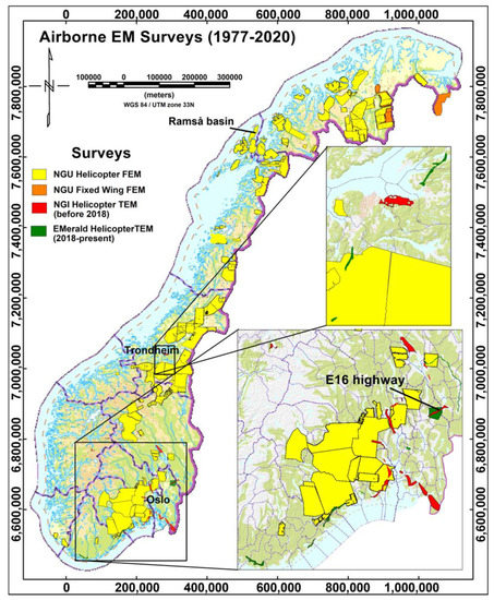
Figure 1.
Helicopter and fixed-wing AEM coverage undertaken by NGU, NGI and EMerald Geomodelling in Norway. Background map from Kartverket [27].
1.2.1. NGU Surveys
NGU has been collecting airborne EM data since 1972, either flying with its own instruments or buying the services from an airborne survey company mainly through various government and municipality-funded projects. The first FHEM system of NGU was a single-frequency SANDER system. NGU started collecting FHEM data at multi-frequencies using an Aerodat EMEX-2; this continued until 1998. The Aerodat system was operated at four frequencies, 915 Hz and 4551 Hz in a co-axial setting, 4287 Hz and 32,165 Hz in a coplanar setting. NGU also collected airborne VLF (very low-frequency EM) data by itself and through other service providers. Some of the VLF data were collected together with FHEM data. NGU bought a five-frequency hummingbird system in 1998 and has been collecting data using this system to date.
The hummingbird system is a similar system as DIGHEMV but operates at different frequencies, i.e., five frequencies, 880 Hz, 6606 Hz and 34,133 Hz in a coplanar setting and 980 Hz and 7001 Hz in a co-axial setting. NGU also bought services for collecting fixed-wing frequency-domain EM and VLF data for few areas in Norway. Fixed-wing FEM data near Norway–Russia border were collected in 1993 at frequencies 256 Hz, 1024 Hz and 4096 Hz. Other fixed-wing FEM data near the Norway–Finland border were collected in 2008–2009 at frequencies of 912 Hz, 3005 Hz, 11,962 Hz and 24,510 Hz. In recent years, NGU collected a large amount of FHEM data through government-funded projects such as Minerals in North Norway (MINN) between 2011 and 2015 and Minerals in South Norway (MISN) between 2014 and 2015, with ongoing efforts through various projects. Reports and details of NGU’s airborne surveys (Figure 1) can be found on the NGU website. Most of NGU’s data are freely available to download from its website and geoscience portal [23].
1.2.2. Norwegian Geotechnical Institute and EMerald Geomodelling Surveys
The first AEM survey undertaken by the Norwegian Geotechnical Institute (NGI) occurred in 2009 to investigate an active rockslide in Western Norway with the ground and airborne resistivity mapping [24]. In the following years, several AEM surveys were conducted for other geotechnical applications, usually connected to large, linear infrastructure projects (i.e., highways, railways, and tunnels). Together, NGI and EMerald Geomodelling have, with the help of SkyTEM, conducted approximately 9850 line kilometers of AEM data from the first survey in 2009 to the end of 2020 (Figure 1).
The AEM surveys were carried out using various versions of the SkyTEM time-domain system; commonly these were the SkyTEM 302 or 304 systems [25]. This choice of system was driven by the needs of geotechnical engineering projects. Broadly speaking, a helicopter-towed system is needed because fixed-wing systems cannot fly as close to the surface or navigate with the same level of precision. SkyTEM systems were specifically chosen because it is an optimal compromise between near-surface resolution and depth penetration. Infrastructure projects in Norway often target shallow and deep investigation targets because the rugged terrain often requires some form of tunneling. Additionally, thick deposits (often upwards of 40 m) of marine clay occur in populated regions of Norway. Stronger signals are required to map depth to bedrock or deposits of sensitive, leached clay because they are needed to penetrate these thick deposits of saline and conductive (usually 5 Ωm or less) material. These constraints are similar to those of groundwater mapping applications of AEM, and SkyTEM’s suitability for hydrogeology (e.g., [26]).
1.3. Coverage Compared to Neighbouring Nordic Countries
Due to steep topography, most of the airborne EM data acquired in Norway are collected by helicopter surveys. Despite the ability of helicopter-based AEM to extend surveys into more challenging regions, this has led to a slowdown in coverage over the whole of Norway and, thus, less coverage of AEM data in comparison to other Nordic countries. Norway has adopted fixed-wing surveys to cover some of the flat regions, but this AEM data was collected in only a few areas. Even so, fixed-wing surveys are not redundant in Norway, though the majority of these that cover larger areas have had a focus on collecting magnetic and gamma-ray spectrometry data, the former of which has coverage over most of Norway [28].
When comparing to neighboring Denmark, Norway’s coverage of airborne-based AEM surveys seems lesser. As of 2015, SkyTEM has collected over 1.5 million soundings, giving close to 40% coverage of Denmark’s onshore landmass. As of 2015, an additional 75,000 ground-based TEM soundings are also available through the GERDA database [29]. Through NGI and EMerald Geomodelling, SkyTEM has collected only 96,575 geophysical soundings over the whole of Norway. For Denmark, this equates to roughly 34 TEM soundings per square kilometer, compared to only 0.25 per square kilometer for Norway. This does not, however, suggest that AEM is a less used method in Norway, but rather that the significantly larger area of Norway has led to a focus on the prioritization of AEM surveying areas rather than a large-scale mapping effort. This would be supported by the fact that both NGI and NGU have played a large role in, for example, quick clay mapping around populated areas [30], or EMerald Geomodelling’s current surveying focus around large-scale infrastructure and engineering projects around highways. The actual geological conditions must be considered as well when comparing the AEM coverage of Norway and Denmark. While Denmark is largely covered by sediments with varying, low resistivities, Norway contains massive areas of mountainous regions with thin, resistive sediments atop resistive bedrock, i.e., little resistivity contrasts to map unless prospecting for mineral deposits. Further, Denmark relies on groundwater as a drinking water source and thus has a strategic interest in understanding the country’s hydrogeology. Soil conditions in Norway are primarily relevant for geotechnical aspects only. AEM has also been widely used in neighboring Sweden and Finland, the former of which adopted AEM earlier than Norway, with surveys starting as early as 1956 where 10,000 km of AEM data were collected [31], and the latter completing nearly full coverage between 1972 and 2004 with fixed-wing surveys. Given the similar geological conditions across Scandinavia, the use cases are similar to those in Sweden and Finland to that of Norway and Denmark, with large-scale clay, groundwater and acidic sulphate soil mapping [32].
2. Material and Methods
Data for this study originates from two case studies of electromagnetic (EM) surveys in Norway.
2.1. Case Study 1—E16 Highway, Southeastern Norway
For our first study, we present data from the proposed re-routing and development of the European Route 16 (E16) motorway between Kløfta and Kongsvinger approximately 60 km northeast of Norway’s capital Oslo. Following the proposal of road improvements, extensive field investigations began in late 2013 across a 30-km segment of roadway in Nes municipality (Figure 2).

Figure 2.
Overview of the E16 survey (see the location in Figure 1) area and underlying quaternary geology. Base map provided by NGU [33].
2.1.1. Geological Setting
The bedrock in the region is predominately comprised of metamorphic rock types, with a smaller area of igneous rocks present towards the northeastern corner of the survey area. Above this, the post-glacial geomorphology is typical for the eastern Norwegian lowlands. Small regions of exposed bedrock and moraines (high electrical resistivity, >1000 Ωm) are common along the road alignment, with areas of glaciofluvial deposits (medium resistivity, 500–1000 Ωm) interspersed. Otherwise, large expanses of glaciomarine clay and marine sediments (very low resistivity, 1–100 Ωm) dominate the survey area [33].
Quick clay, a complicated geological hazard common to the lowlands of southeastern Norway, is present in this area. Quick clay forms by freshwater leaching of glaciomarine clay. In Norway, it is defined as clay with a remoulded shear strength below 0.5 kPa. Though stable when undisturbed, erosion or human activities that disturb such deposits can cause dramatic landslides. In Norway, extensive quick clay hazard and risk mapping has been carried out by NGI and others, coordinated and financed by the Norwegian Energy Directorate (NVE), who holds the national responsibility of natural hazard mapping and risk management. The various possible road corridors traverse several known and mapped quick clay hazard areas, and further deposits are likely to exist outside those that have been detected thus far.
2.1.2. Geophysical Data
In January 2013, 178 line-km of AEM data were flown along the planned road alignment. As this was a pilot project, the smallest system (SkyTEM 302) was used to allow for the highest depth resolution from the fastest turn off times. In 2020, an additional 5 areas of interest were scanned with a total 529 line-km flown (Figure 2) using the SkyTEM 304 system [25]. Flying with the EM-sensor 30 m above the ground, this system measures electromagnetic induction effects from the ground, with penetration depths ranging from 50 m to 300 m into the ground depending on geological conditions. The first usable gate was gate 6, with the center time at gate 6, at 1.022 × 10⁻⁵ s, and the last possible gate being gate 32, with a center time of 3.544 × 10⁻³ s.
With the specialized software Aarhus Workbench, both datasets were then processed and cleaned for noise and coupling effects from infrastructure. Using inversion modelling, a pseudo-3D resistivity model was then produced via a spatially constrained inversion (SCI) [34], with a vertical resolution ranging from meters close to the surface to tens of meters at greater depths. The lateral resolution for such models is, however, larger, with a range between 50 m to 150 m [35]. The inverted resistivity models are then interpolated to a 3D grid by ordinary kriging [36] to be used as needed for further modelling.
2.1.3. Geotechnical Data
Throughout this paper, we interchangeably refer to geotechnical investigations as: boreholes, geotechnical soundings and drillings. Large-scale geotechnical investigations were also undertaken around the survey area. During 2013, almost 1400 geotechnical soundings were performed along the central part of the survey area (Figure 3). It was found that 1105 soundings had a measurement of depth to bedrock, and of these, only 98 were total soundings, which were drilled at least 3 m into rock to confirm bedrock. The remaining 1007 drillings were rotary pressure soundings (DRT), which typically stopped when reaching hard material assumed to be bedrock. DRT depths thus may be depth to bedrock, but could also be depth to other material such as glacial erratics or hard moraines. A total of 1387 DRT soundings were undertaken at 1379 locations, with 762 of these locations within the 75 m footprint of AEM measurement points. An additional 27 boreholes were within the survey area from 2020, and a further 45 were drilled during August 2020 in the south of the 2020 survey area. Of these 45, 26 had a confirmed depth to bedrock though only 15 were within 75 m of an AEM point.
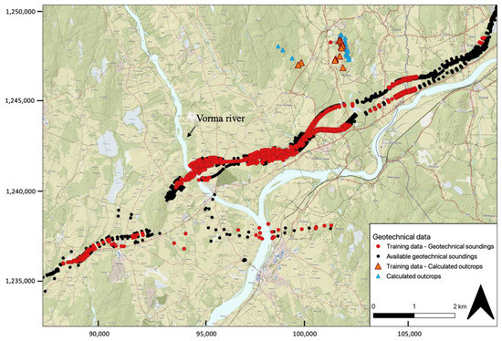
Figure 3.
Geotechnical data around the E16 AEM survey (see the location in Figure 1). Coloured circles denote geotechnical sounding data, coloured triangles denote locations of calculated outcropping bedrock. The topographical background map available from [37].
We also used a high-resolution digital terrain model (DTM) with 1-m grid spacing to calculate areas of likely outcropping bedrock (Figure 3). Areas in which the slope length was greater than 3 m at an angle exceeding 45 degrees were deemed to be outcropping bedrock. These points were then manually checked, using high resolution satellite imagery to ensure false positives were removed from the dataset. Outcrops that were within 75 m of an AEM measurement point were included as training data for the bedrock model. An overview of all training data is seen in Table 1.

Table 1.
Overview of training data used in the artificial neural network for bedrock modelling.
An additional 1980 soil samples were taken at parts of those sounding locations. Lab measurements of remolded shear strength were made at different depths at 88 different locations. Over 99% of these were in clay material. Of these samples, 58 were not used in the quick clay machine learning algorithm (discussed later in this section) due to data quality questions. From the remaining 1922 samples, roughly 16% were quick, 17% were brittle but not quick and 66% were non-brittle (Table 2).
Table 2.
Overview of soil sample data used in the quick clay analysis.
2.1.4. Depth to Bedrock Modelling
We use an artificial neural network (ANN) to predict the location of the top of bedrock. This choice is the result of comparisons of multiple interpretation methods on similar projects in Norway since 2013. A simple contouring of resistivities led to poor results in this project back in 2013 due to spatial variations in the resistivity corresponding to the top of bedrock [3]. Automated approaches such as geostatistical modelling [38], linear transforms like the Linear Smart Interpolation (LSI) [39,40], and ANNs [41] have been tested since then. ANNs tend to have the best performance [41,42], even with only sparse geotechnical data, because they can adjust for local variations in bedrock resistivity and changes in geological environment. A back-analysis of the 2013 data showed that with 50 boreholes, the ANN-generated top of bedrock model had a median absolute error of 4.0 m (24% of depth) compared to 6.0 m (43% of depth) for the best-performing contoured surface of 100 Ohm m and 4.6 m (28% of depth) for the model manually interpreted by geophysicists at the time [40].
To prepare the input data for the ANN, we first interpolated a vertical resistivity model to geotechnical sounding locations using ordinary kriging, similar to [36]. We excluded boreholes located more than 75 m from AEM data locations given that this is roughly the size of the footprint of the AEM instrument. These collocated bedrock measurements and interpolated resistivity constituted the training dataset to the ANN. The resistivity model layers and the spatial coordinates (X, Y, and Z) were used as features, and the depth to bedrock was the target label. Spatial attributes are commonly included in this sort of predictive geological modelling (e.g., [43,44]). Note that where geotechnical soundings are not present, manual interpretation points of the geophysical model can be used instead as training data.
We use a feed-forward, multi-layered perceptron regressor implemented in scikit-learn, a Python module [44]. Weighting parameters within the network are randomly initialized, and training proceeds using the Limited-Memory Broyden–Fletcher–Goldfarb–Shannon (L-BFGS) optimization algorithm [45]. The target loss function has two terms: the L2 norm of data misfits and a regularization term penalizing large variations in ANN weights. The relative strength of regularization is tuned manually by users to find the right balance between over- or underfitting based on a visual inspection of output models. Uncertainties are estimated by repeating predictions with multiple networks and computing the variance of output predictions.
2.1.5. Quick Clay Modelling
Both the remoulded shear strength and the electrical resistivity of quick clay are strongly correlated to their salt content, lending themselves well to mapping using electromagnetic methods. However, the resistivity signature of quick clay is non-unique. Whereas material that with very high (>100 Ωm) or very low (<5 Ωm) can be ruled out as quick, marine clay with intermediate resistivities may either be leached, quick marine clays, or marine clays that was mixed with coarser sediments or which has undergone weathering processes [46]. Intrusive geotechnical investigations are needed to resolve this ambiguity.
We use a two-step modelling approach introduced by [47] and refined by [48] to predict the probability of quick clay. In the first step, laboratory tests, wherein remoulded shear strength has been measured directly, is used to train a random forest classifier interpret the presence of quick clay at geotechnical sounding locations. This step is necessary to create a balanced training dataset; lab samples tend to be biased towards quick clay deposits, whereas geotechnical soundings and the AEM data sample a wider range of sediment types. Using the automatically interpreted geotechnical soundings and lab data, a second random forest classifier is used to predict the probability of quick clays on volumetric grid of electrical resistivities. Both classifiers are implemented with the scikit-learn Python module [44].
2.2. Case Study 2—The Ramså Basin, Northern Norway
The Ramså Basin in North Norway is the only known Mesozoic basin in onshore Norway. It is situated along the strandflat on the northeastern side of Andøya between Ramså and Skarstein. Its thickness is claimed to be more than 650 m [49]. Deeply weathered materials are exposed at the surface [50] and were also observed in well cores drilled in the Ramså Basin [49,51]. A bedrock map of the area surrounding Ramså Basin is shown in Figure 4. The primary basement rocks in the region are mainly granodiorite, granite and gabbro. The sedimentary rocks in the Ramså Basin consist of sandstone and different variations with clays and shales of the mid-Jurassic to the early Cretaceous age [49,51]. A few bands of quartzite are also observed as part of super crustal metasedimentary rocks in the Skogsvoll group, south of the Ramså Basin. The original boundary of the Ramså sedimentary basin is derived from [52], which was refined using shallow drilling information [51,52,53,54] and is shown by the green line in Figure 4.
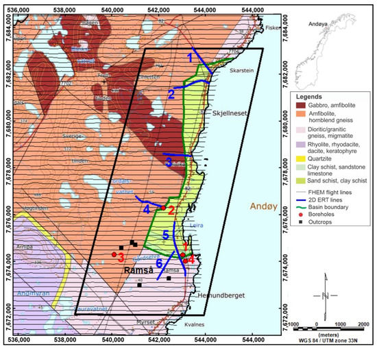
Figure 4.
Bedrock map of the area surrounding the Ramså Basin [52] with locations of FHEM flight line, ERT profiles, boreholes and observed outcrops. The originally assumed western extent of the Ramså Basin is shown by green line.
A helicopter survey to collect airborne geophysical data from the whole of Andøya island was performed in 2012 [55]. Six electrical resistivity tomography (ERT) profiles (blue lines in Figure 4) were collected in 2010 using the LUND system [56] and multigradient electrode configurations [50]. Later, four boreholes (red circles in Figure 4) were drilled and logged using Robertsson Geologging equipment in 2015 and 2016 [57]. The locations of these boreholes were chosen based on the initial interpretation of the geophysical data. A few exposed bedrock observations are also shown by black squares, and thin black lines in E–W direction show FHEM flight lines. FHEM data at five frequencies were collected at ca. 200 m line spacing and at 56 m average sensor altitude. Three coplanar frequencies of FHEM data from a smaller area (black parallelogram in Figure 4) out of the larger helicopter survey were inverted using an SCI to obtain true subsurface resistivity. Details of the inversion strategy are discussed in [58]. The subsurface resistivity model from this smaller region is discussed in the results section.
3. Results
3.1. Case Study 1—E16, Nes County
We highlight three main results in the following subsections. First, we generate predictions of top of bedrock over the 2013 survey area using an increasing number of boreholes (Section 3.1.1). Next, we predict depth to bedrock in the new 2020 survey areas and compare with later boreholes (Section 3.1.2). Finally, we compare our predictions of quick clay occurrence to existing hazard maps (Section 3.1.3).
3.1.1. Bedrock Modelling (2013 Survey Area)
A bedrock model produced with only five boreholes captures large-scale trends in bedrock topography relatively well. Some features one might expect, such as a reduction in bedrock elevation under rivers such as the depression under the river Vorma that is predicted to be ca. 40 m lower than surrounding areas (Figure 5A) are evident. Using an additional 20 boreholes to produce a bedrock model clearly delineates large-scale features further, as topographic highs and lows become more detailed, with a noticeable separation in the large region of lower bedrock elevations in eastern regions into two separate topographic lobes.
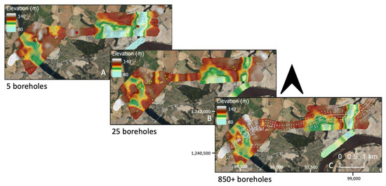
Figure 5.
The evolution of a bedrock model from a central section of the 2013 survey area. (a) Five boreholes, (b) 25 boreholes and (c) 850+ boreholes used as training data. Adapted from [41] Background map from Google Satellite Imagery [59].
On a large scale, a bedrock model training on over 850 geotechnical soundings only adds to the topographic ‘resolution’, in that high and low features become more exaggerated when compared to the model from five boreholes. This shows that the effect of the additional boreholes serves to improve the areas where the 5 and 25 borehole models lack information, in regions of particularly high or low bedrock elevation where they lack training data that would justify such extremes. Even with these extremes, a five borehole bedrock model prediction evidently produces a representative early-stage view of subsurface conditions. These results emphasize the benefits of using a neural network and AEM to predict bedrock surfaces, both producing excellent insight early on in a survey and reducing the need for expert geophysical or geotechnical information through hundreds of boreholes. An extensive study of the increase in accuracy for this and one more site is provided by [34].
3.1.2. Bedrock Modelling (2020 Survey Area)
The first depth to bedrock model for the 2020 survey areas was produced by training an ANN using existing 2013 AEM survey data, all existing 850+ boreholes, as well as a small number of manual interpretations within surveyed areas. This prediction was then compared to the first 15 geotechnical soundings within the survey area that confirmed depth to bedrock (Figure 6, Table A2 of the Appendix A). The larger magnitude of prediction errors tended to occur for deeper holes. The largest mismatch of +22.25 m is seen from the predicted depth to bedrock of 45 m, whereas holes shallower than 20 m have a prediction error is less than +/−3 m (Figure 6A). The minimum prediction error was 0.14 cm (Figure 7, Borehole 7-0u, 1400 m distance along line). The mean magnitude of prediction error was 25% of depth, with the minimum and maximum error normalized by depth being 0.003 and 0.52. These occur at 35 m and 32.3 m depth, respectively (Figure 6B). An illustrative cross-section showing the resistivity model, predicted depth to bedrock, and new boreholes is given in Figure 7.
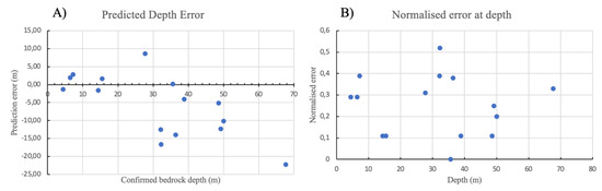
Figure 6.
(A) Predicted depth error between bedrock confirming boreholes and the ANN produces bedrock depth predictions for the 15 geotechnical drillings in the ground-truthing dataset. (B) Errors normalized by confirmed depths for the same set of boreholes.
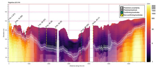
Figure 7.
2D cross-sectional view of a flight line from the inverted AEM model, showing boreholes drilled in October 2020 confirming bedrock (green) and non-bedrock confirming boreholes (yellow) against the predicted bedrock surface from July 2020. Borehole labels show borehole ID, depth drilled and distance from an AEM sounding. Areas of increased transparency indicate the model is below the depth of investigation.
To evaluate the accuracy of the prediction uncertainty estimates, we compute a metric we call the error ratio:
Nine of the 15 geotechnical soundings that confirmed bedrock had an error ratio below 1 (Figure 8). Generally, the uncertainty was overestimated where bedrock was shallow (<15 m depth), but errors were greater than expected for deeper areas.
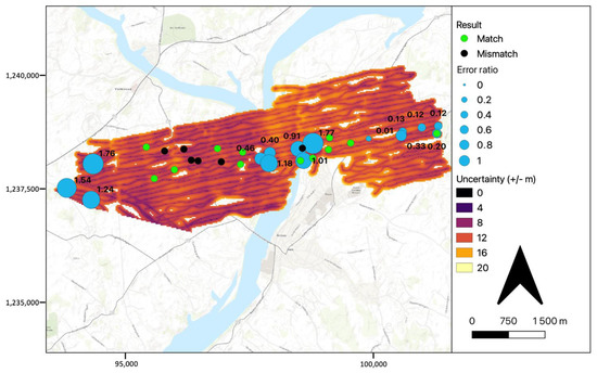
Figure 8.
Error ratios for geotechnical soundings versus predicted bedrock depth uncertainty for boreholes confirming a bedrock depth (blue circles), and matching (green circles) or mismatching (black circles) geotechnical soundings. Background map from [27].
In addition to bedrock-confirming boreholes, 18 boreholes were drilled that did not reach bedrock. We considered boreholes that were within the uncertainty of the predicted bedrock interface as a “match” and boreholes that were drilled deeper than our predictions, including uncertainty as a “mismatch”. We found 12 matches and six mismatches among this ground truth data (Figure 8).
3.1.3. Quick Clay Modelling
The project area is situated in the southeastern Norwegian lowlands that are prone to the existence of quick clay, a complicated geological hazard. Quick clay forms by freshwater leaching of glaciomarine clay are classified as having extremely low remolded shear strength (under 0.5 kPa) and thus causes dramatic landslides when disturbed. In Norway, extensive quick clay hazards and risk mapping has been carried out by NGI and others, coordinated and financed by the Norwegian Energy Directorate (NVE), which holds the national responsibility of natural hazard mapping and risk management. The various possible road corridors traverse several known and mapped quick clay hazard areas and further deposits outside of mapped areas are likely.
In the central regions of the 2013 survey area, several bodies of mapped quick clay overlap the regions with AEM data, with the majority of the zones classified as middle or high probability of a quick clay slide (Figure 9). For the whole survey area, the predicted quick clay thickness from our algorithm range from 0.3 m–39.3 m. We note that these have no bearing to what depth quick clay is predicted to be found at, but instead the total volumetric prediction for a vertical column on a 20 m × 20 m grid. Our quick clay predictions show that areas of thicker clay (greater than 20 m) were commonly found in regions identified as ‘middle’ or ‘high’ risk by NVE. Care must be taken when potential quick clay thickness is compared with hazard zones. Quick clay hazard zones are classified based on a multitude of factors, including slope angle and extent, erosion potential and geotechnical properties including quick clay thickness. Note that the geophysics-based prediction indicates an extension of quick clay regions outside of the mapped hazard zones. Though these are generally predicted to be in areas of thinner quick clay predictions, regions of quick clay between 20 m–25 m thick are found in un-recognized quick clay risk zones (black squares, Figure 9).
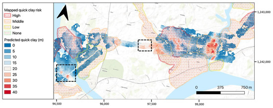
Figure 9.
Mapped risk of quick clay landslides by NVE [60] compared to predicted quick clay thicknesses. Black squares show regions of thicker predicted quick clay not previously mapped by NVE and NGI. Background map from [27].
3.2. Case Study 2—Ramså Basin
This section briefly describes subsurface resistivity model from NGU’s FHEM data and its validation. A comparison of resistivity obtained from FHEM with resistivity from ERT and borehole logging at four borehole locations is presented first. Then, a 3D resistivity model of onshore Ramså Basin and its surroundings is presented to show a possible extension of the sedimentary basin.
3.2.1. Comparison of Subsurface Resistivity from FHEM, Borehole and ERT
Four boreholes were located along different flight lines of the helicopter survey. Inverted resistivity obtained from an SCI of FHEM data were extracted from the borehole locations to compare it with the resistivity obtained from borehole logging and ERT. A comparison of three resistivities is presented in Figure 10. We observed a good correlation among them at all four borehole locations with a varying range of resistivity between ca. 10 Ωm and 2000 Ωm. Similar resistivity values at four borehole locations shown by the FHEM, ERT and borehole logging establish the validity of the FHEM inversion results. The resistivity of the water in the boreholes and interpreted geological formation log is also added in the figure for each borehole, and the upper 10 m–20 m of boreholes were cased. Reported geological formations were defined on the basis of their geological age and analyses of the drill cores [57]. All the formations shown here belong to the Ramså sedimentary basin except the basement. Borehole (or formation) resistivity is controlled by the porosity of the formation, its saturation and salinity/conductivity of the pore water. Resistivity variations within the boreholes correlate well with the water resistivity variation in the borehole. Water resistivity measured in boreholes 1 to 3 is found very close to seawater resistivity. The borehole resistivity varies between 100 Ωm–500 Ωm within the first 10 m–20 m of basement rock, most likely due to the presence of conductive pore water in the fresh bedrock and the weathered bedrock, while outcropping bedrock in borehole 4 is logged around 1000 Ωm. The resistivity range of 100 Ωm–500 Ωm is also depicted by the sedimentary basin at the surface, where it is likely to be saturated with fresh pore water as seen in borehole 1 and 3. Weathered basement was observed at the surface at few locations, with core logging from borehole 4 confirming that this location was outside the Ramså Basin. Low resistivities from FHEM below 50 m in borehole 4 could be due to conductive water or minerals in a fractured basement. Borehole resistivity of the sedimentary basin varies between 10 Ωm and 600 Ωm at depths, though it becomes less than 300 Ωm below 30 m depth.
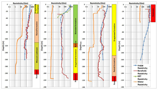
Figure 10.
Comparison of resistivities obtained from FHEM, borehole logging and ERT at four borehole locations for borehole 1, 2, 3 and 4 (from left to right). Water resistivity in the boreholes and interpreted geological formations are also shown in the figure (reproduced after [58]).
3.2.2. 3D Resistivity Model of the Ramså Basin
Horizontal resistivity slices interpolated from the SCI of FHEM data are shown at various depths in Figure 11. The Ramså Basin in the top two slices (at 2 m and 20 m depth) is relatively resistive (500 Ωm–600 Ωm) compared to the resistivity of the basin at greater depth (<300 Ωm). Highly conductive seawater and possible marine sedimentary rocks are seen in the east. The basement rock seems to be highly fractured as moderate to high conductive areas (green and blue colored) show up below and in the middle of highly resistive basement (yellow to red-colored). The resistivity does not show a regular increase with depth, to indicate the transition from fractured to fresh bedrock. Rather, it shows an opposite behavior of showing higher conductivity with depth. Borehole logging also reported a lower conductivity of the borehole water at a shallower depth and higher conductivity at greater depth at all the four borehole locations. The basin is more conductive at depth, and it could be filled with conductive seawater.

Figure 11.
Resistivity slices at 2 m, 20 m, 45 m, 76 m, 118 m and 150 m depth below the surface obtained from SCI of three coplanar frequencies (880 Hz, 6606 Hz, 34,133 Hz) from the black parallelogram area (Figure 4). The Ramså Basin boundary, borehole and outcrop locations are also marked with the same symbols as in Figure 4. Contours lines of 300 Ωm (outer contour line) and 100 Ωm (inner contour line) are plotted with black lines (modified after [58]).
Figure 11 shows changes in resistivity near the basin boundary in the resistivity slices, which indicates that the basin boundary changes at depths. Resistivity variation within the basement area due to significant fracturing of the basement was confirmed by well logging resistivity and core samples. However, the FHEM inversion could not resolve deeper than ca. 150 m and consequently does not resolve the basin base to show an expected more pronounced contrast of resistivity between basin and weathered/fresh bedrock.
3.2.3. Possible Extension of the Ramså Basin
The original Ramså Basin extension was drawn mainly based on earlier geological surface observations and shallow drillings, with only sparse geophysical data coverage available at that time. Recent airborne magnetic, FHEM, gravity, ERT and 2D seismic surveys helped to re-explore the area and to redraw the Ramså Basin boundary [61]. Borehole location 3 was considered outside the sedimentary basin according to the earlier geological interpretation but recent geophysical survey results suggest that the basin extends at least to this location, and it is confirmed by core samples obtained from borehole 3.
FHEM, borehole logging and ERT profiles in the area show a resistivity range of ca. 10 Ωm–300 Ωm for the Ramså Basin below ca. 30 m depth. Therefore, contour lines of 300 Ωm and 100 Ωm are plotted with black lines on top of the resistivity slices (Figure 11) to identify the boundary of the Ramså Basin. The contoured regions (outer and inner contour lines are 300 Ωm and 100 Ωm, respectively) show weathered rocks and the sedimentary basin together. Basement outcrops observed near the location of borehole 3 between 45 m to 150 m depth are situated between the 100 Ωm and 300 Ωm contour lines. Magnetic and gravity data interpreted this part of basement outcrop to be a horst [61]. FHEM data shows 300 Ωm–600 Ωm resistivity from surface to 45 m depth and <300 Ωm below 45 m depth for this area.
Borehole location 3 (inside sedimentary boundary as confirmed by drilling cores) and outcrop observations near borehole 3 (outside of the sedimentary basin) could be separated by ca. 400 Ωm resistivity boundary at the surface. If the basement is continued to be present at greater depths, then this part of the basement shows a low resistivity of ca. 200 Ωm. A discontinuity of 100 Ωm–300 Ωm resistivity around the outcrop observations near borehole 3 with the rest of the basin depicting resistivity < 100 Ωm is observed in the resistivity slices from 45 m to 150 m depth (Figure 11). The 100 Ωm contour lines could separate the extended basin in two parts at basement outcrop observations (between 45 m to 150 m depth) to match with other geophysical and outcrop observations. Therefore ca. <100 Ωm resistivity seems to be appropriate for this part of the Ramså Basin from 45 m to 150 m depth and shows the basin extent well. The lateral extent of the sedimentary basin beyond the borehole 3 location should be confirmed by additional borehole and geological observations. Borehole 4 is confirmed to be outside of the sedimentary basin from drilling cores. It should be noted that EM and other resistivity methods alone cannot distinguish between fractured and weathered basement or basin sediments with similar resistivity.
4. Discussion
4.1. Synthesis of Case Studies
Case study 1 demonstrates the utility of using AEM for geotechnical site investigations and of combined geotechnical and geophysical data into an integrated modelling process. Our comparison of bedrock models using differing numbers of input training boreholes (Section 3.1.1) showed that using AEM can give early insight into broad geological structures without the need for extensive drilling campaigns. Although increasing the number of boreholes increases the level of detail in the bedrock model, even with only 5 boreholes, we detected, among other features, deep bedrock channels below rivers. Our quick clay modelling (Section 3.1.3) both agreed with deposits of quick clay previously mapped by NVE and also pointed to other locations where quick clay is plausible (Figure 9). These outcomes are valuable for early-phase planning of large infrastructure projects.
The prediction accuracy of our machine-learning methods is on par with our expectations, but there is still room for improvement. In the new 2020 survey, predictions on average deviated from new boreholes by 25% of depth, similar to the back-analysis performed on the 2013 project areas [41]. This is the first time we compare uncertainty estimates to prediction errors. Measured depth to bedrock was within predicted uncertainties for 60% of bedrock-confirming holes and 67% of non-confirming holes. These are approximately the proportions we would expect for one standard deviation of a normal distribution. While this is a promising result, these estimates fall short because they overestimate uncertainty in shallow areas and underestimate it for deep areas.
We can attribute some of the prediction errors in the new 2020 survey areas (Figure 8) to several factors. In western portions, geological investigations show a mixture of thick marine deposits and fluvial deposits, whilst surface water bodies like the river Glomma have resistivities that overlap with those of (conductive) sediments. Both of these factors can reduce contrast through the vertical layers of the inverted AEM model, reducing the accuracy of the ANN predictions. These effects are also likely exacerbated by the lack of geotechnical training data in the locale.
Case study 2 in turn demonstrated how frequency domain AEM is also a useful tool in the mapping of a sedimentary basin, with results allowing the prediction of a possible extension of the Ramså Basin. It could not confirm the depth of the bedrock due to the limited depth of investigation as a result of the frequencies used (and therefore skin depth) in the Hummingbird system. A different system such as a SkyTEM instrument, could have revealed deeper subsurface investigations conditions down to 500 m below the surface. Lateral and depth resolution of quick clay and marine clay layers at shallow depth (down to 10 m–100 m) were resolved better by the Hummingbird system than the SkyTEM system from a case study from Numedalen Valley, Norway [62].
The example from the Ramså Basin shows AEM’s ability to find out the lateral extent of the sedimentary basin. However, the same resistivity could also be attributed to fractured bedrock with seawater and weathered geological units. An SCI, being a quasi-3D inversion (with a 1D forward modeling), could produce a resistivity model to match with ERT and borehole resistivity because the area is represented by sufficiently large horizontal layers (few hundred meters on the surface) without strong local 3D effects. An AEM inversion is an ill-posed problem like other geophysical inversion and there could be infinite solutions to it. A different starting model, regularization parameter, or lateral and vertical constraints in the inversion modelling may lead to a completely different inverted resistivity model. Therefore, sensitivity analysis of the inversion model, ground-truthing and additional information from other geophysical and geological observations are necessary to validate it.
4.2. Generalizations: Advantages and Limitations of AEM for Ground Investigations
We see the main advantages of using AEM to perform ground investigations falling into two main categories: (1) data coverage and time savings, and (2) cost savings.
Exemplified by case study 1, using AEM methods benefit from the ability to cover vast areas in extremely short amounts of time. For this case study, nearly 600 line kilometers of geophysical information was collected in less than five days, with an initial bedrock topography model extracted only five days later. Depending on the EM acquisition system, it is not uncommon to acquire up to 500–1000 line kilometers of data per day [63]. Achieving equal lateral coverage with traditional methods such as in-situ drillings would not be feasible. Though lateral coverage is determined by both flight path and flight height, AEM, with adequate survey planning can provide seamless coverage over a given area. Although drillings can go deeper than AEM, the vertical coverage (depth penetration) of AEM is similarly advantageous. With the correct system, subsurface information can be collected down to 1000 m depth, and semi-airborne methods such as GREATEM are even capable of extending this down to 1500 m [16]. The only factor that can prevent seamless coverage is from infrastructure, which may cause couplings or prevent a safe flight path, or particularly hazardous topography.
When working over large areas, AEM surveys become a cost-effective method, particularly as an early-stage solution for reconnaissance or a tool for investigating potential areas of interest. Bedrock modelling has historically been done through a simple triangulation of boreholes. Though this reduces uncertainty at spot locations, the amount of geotechnical information required to produce a detailed model can take years to collect and is expensive to conduct. It has been estimated that a single borehole to 20 m depth can cost 8620 NOK (EUR 827, USD 980), and a single line kilometer of AEM data around 4830 NOK (EUR 463, USD 549) [3]. Though bedrock depth is not easily inferable from an inversion model, the cost can be nearly half as much for significantly more data than a single point with bedrock depth. With an integrated method, such as using AEM with an ANN for bedrock modelling, the number of geotechnical drillings needed is, and therefore the cost of ground investigations, rapidly reduced.
These advantages can explain why the use of AEM in Norway has expanded in recent decades from mineral exploration to more engineering and environmental applications. While AEM still continues to be used for mineral exploration (e.g., [6,7,64]), both TEM systems [9,48] and FEM systems [10,11] have been successful in mapping quick clay occurrence. In fact, both ground-based and airborne resistivity imaging methods are now recommended as tools for large-scale quick clay mapping [65].
However, AEM has several limitations on its utility for ground investigations. First, the resolution is rather low and may not always be sufficient for all applications, though efforts are ongoing to extract early-time/high-frequency signal to improve near-surface resolution [66]. Second, accounting for 3D effects is computationally intensive, meaning that the most commonly used inversion schemes result in models with a high degree of lateral smoothing. Third, AEM data give little added information when there is not resistivity contrast between two target units.
Yet, despite these weaknesses, the case studies in this paper show that ground models of reasonable accuracy can be acquired by combining inverted resistivity models with ground truth data. Where the resistivity model is ambiguous or lacks contrast, ground-truth data helps resolve the unknown. Using high-resolution intrusive investigations helps one recover detailed features in the subsurface. Other authors have noted that machine learning algorithms achieve this largely by way of the spatial coordinates [43,48], emphasizing the need for local ground-truth data. Beyond the correlative analyses and machine learning algorithms explored in this paper’s two case studies, other integrated modelling approaches used outside of Norway include using multiple-point statistics for stochastic stratigraphic modelling [67,68,69], and local neighbourhood statistical analysis [69]. Even with these support data, the model does have a high degree of uncertainty at locations where there are no ground truth observations, so AEM, for now, remains most valuable in early phase ground observations where precision is not yet critical.
4.3. Future Trends
Globally, AEM instrumentation has developed rapidly, with almost continuous year on year advancements in acquisition and hardware systems, calibration methods and data processing routines largely driven by the introduction of TEM to hydrogeological investigations [16]. These developments mean more systems are available, and therefore systems exist that would allow one to investigate near the surface (0 m–150 m) or down to ca. 1 km below the surface [16].
It is with these developments and widespread adoption that the future direction of AEM both in Norway and globally is expected to continue on the same trajectory since its development in the 1950’s. As systems become more compact, the use of drones is likely to reduce the dependency on costly helicopter and fixed-wing methods, whilst also increasing the use of AEM to smaller study sites, more remote locations and most significantly, collecting higher resolution data. Drone-Borne Electromagnetic (DREM) has already proved successful for the effective mapping of shallow groundwater and surface water salinity [70].
Methods have been tested with promising results showing that real-time inversions of airborne TEM data using an ANN can provide at least equal quality inversions as standard 1-D deterministic methods. Here, an inversion could be completed in only 24 s using a standard laptop, compared with an inversion taking a few hours using standard inversion methods [71]. Such developments could significantly change typical survey conduction, as real-time data allows for real-time interpretation to a given survey. With these continued technological advancements and machine learning algorithms in mind, such as those used to accurately predict depth to bedrock or quick clay deposit volumes and mineral exploration, it can be assumed that AEM coverage and demand will increase in Norway and globally in the coming years. Probably one of the most visionary current initiatives globally is Australia’s AusAEM program aiming at covering the vast continent of Australia with AEM at regional resolution to identify major structures pointing towards minerals and groundwater resources [72].
5. Conclusions
With the aid of two case studies, we have demonstrated the applications and benefits of using AEM data in subsurface investigations. AEM provides a rapid acquisition method to cover significantly larger areas than common ground-based surveying methods in a short amount of time. Their used cases are broad and add significant value from applications such as hazard mapping, engineering projects, resource discovery or simply improved geological mapping from the surface to several hundred meters below.
AEM data alone can provide detailed answers of large-scale subsurface features and even lithological properties, though the addition of external data such as geological mapping and geotechnical soundings will provide greater subsurface information when combined with AEM data. The technological advancements in AEM hardware and development of machine learning algorithms have allowed AEM data to be used for accurate tools such as bedrock prediction and hazard (quick clay) predictions.
In Norway, AEM coverage is perhaps more sparse than other Scandinavian countries such as Denmark, though this is assumed to be a result of geographic conditions. These geographic conditions have influenced its use within Norwegian industry and the methodological choices of system, survey design, and data processing. These lessons may help other countries with similarly rugged terrain or complex post-glacial geology.
With the benefits AEM surveys provide and the increasing use of drones and continuous technological development, we expect the use of AEM methods for ground investigations to remain a key tool for remote sensing in both Norway and the world in the coming years.
Author Contributions
Conceptualization, E.J.H., V.C.B., A.A.P., J.S.R., M.B.; methodology, E.J.H., V.C.B., C.W.C.; software, C.W.C., V.C.B.; formal analysis, E.J.H., V.C.B., C.W.C.; investigation, E.J.H., V.C.B., C.W.C.; data curation, E.J.H., C.W.C., V.C.B.; writing—original draft preparation, E.J.H., V.C.B.; writing—review and editing, E.J.H., V.C.B., A.A.P., C.W.C., J.S.R., H.A., M.B., G.H.S.; visualization, E.J.H., V.C.B. All authors have read and agreed to the published version of the manuscript.
Funding
This research received no external funding.
Institutional Review Board Statement
Not applicable.
Informed Consent Statement
Not applicable.
Data Availability Statement
Case study 1: Geophysical data sharing not applicable. Data was obtained from Emerald Geomodelling AS, but is owned by the Norwegian Public Roads Administration. Publicly available geotechnical data excluding that collected in 2020 regions of cast study 1 can be accessed and downloaded from the National Database for Ground Investigations (NADAG). This data can be found here: http://geo.ngu.no/kart/nadag-avansert/ (available in Norwegian only). Case study 2: NGU data is publicly available from the NGU website and detailed interpretations and plots can also be obtained on request from Authors.
Acknowledgments
We want to thank the Norwegian Public Roads Administration and all the project partners of Ramså Basin project for allowing us to use the data in this study.
Conflicts of Interest
The funders had no role in the design of the study; in the collection, analyses, or interpretation of data; in the writing of the manuscript, or in the decision to publish the results.
Appendix A
Table A1.
A compilation of case studies of AEM projects in Norway and associated publications.
Table A1.
A compilation of case studies of AEM projects in Norway and associated publications.
| Location | Survey Dates | Description | System | Use Cases | Related Publications | |||||
|---|---|---|---|---|---|---|---|---|---|---|
| Depth to Bedrock | Soil Properties (Including Quick Clay) | Landslide Hazard Assessment | Weakness Zones | Mineral Prospecting/ Graphite/ Uranium | Rock Unit Mapping | |||||
| Flåm Valley, Aurland municipality | 2009 | Landslide hazard study | SkyTEM | x | [24,73] | |||||
| Kløfta-Kongsvinger | 2013, 2020 | Road planning project for the E16 highway | SkyTEM | x | x | [9,38,41,47,74] | ||||
| Gran and Jevnaker | 2014 | tunneling and road cuts through hazardous black shale | SkyTEM | x | [14] | |||||
| Brumunddal-Lillehammer | 2015 | railway corridor planning (InterCity project) | SkyTEM | x | [75] | |||||
| Various railway corridors around the Oslo fjord, eastern Norway | 2015 | railway corridor planning (InterCity project) | SkyTEM | x | x | [76,77] | ||||
| Sandvika-Hønefoss | 2016 | Joint road and railway planning project for E16 highway | SkyTEM | x | x | x | x | [40,78] | ||
| Gulskog-Hokksund | 2016 | Railway planning project west of Drammen | SkyTEM | x | x | [41] | ||||
| Trøndelag county | 2019 | Road planning for E6 highway for multiple segments near Trondheim | SkyTEM | x | x | x | x | [48,79,80] | ||
| Kongsberg | 2009 | Alum shale/uranium exploration | NGU Hummingbird | x | [81,82] | |||||
| Numedalen | 2006, 2010 | A comparison of SKYTEM and Hummingbird data interpretation | NGU Hummingbird | x | x | [64] | ||||
| Byneset | 2012–2013 | Quick clay mapping | NGU Hummingbird | x | x | x | [11,83] | |||
| Andoya | 2012–2015 | Basin extension and bedrock depth | NGU Hummingbird | x | x | [59] | ||||
| Northern Norway | 2012–2016 | Graphite exploration | NGU Hummingbird | x | [62,84,85] | |||||
Table A2.
An overview of the ground truthing dataset, showing the depth of confirmed bedrock, the predicted depth at this borehole location, the difference, the uncertainty of the prediction and the error ratio.
Table A2.
An overview of the ground truthing dataset, showing the depth of confirmed bedrock, the predicted depth at this borehole location, the difference, the uncertainty of the prediction and the error ratio.
| Borehole ID | Bedrock Depth (m) | Predicted Bedrock Depth (m) | Difference (m) | Uncertainty (m) | Error Ratio |
| 1-0u | 4.43 | 3.13 | −1.29 | 11.18 | 0.29 |
| 2-0u | 6.40 | 8.28 | 1.88 | 9.54 | 0.29 |
| 5-0u | 7.20 | 10.03 | 2.83 | 8.47 | 0.39 |
| 4-0u | 14.40 | 12.82 | −1.58 | 12.65 | 0.11 |
| 3-0u | 15.48 | 17.12 | 1.65 | 13.33 | 0.11 |
| 13A-0u | 27.73 | 36.33 | 8.60 | 9.46 | 0.31 |
| 33-0u | 32.15 | 19.67 | −12.48 | 8.10 | 0.39 |
| 31-0u | 32.30 | 15.64 | −16.66 | 9.45 | 0.52 |
| 7-0u | 35.58 | 35.72 | 0.15 | 12.35 | 0.00 |
| 32-0u | 36.40 | 22.44 | −13.96 | 11.27 | 0.38 |
| 15-0u | 38.83 | 34.71 | −4.12 | 10.41 | 0.11 |
| 17-0u | 48.58 | 43.37 | −5.20 | 11.27 | 0.11 |
| 16-0u | 49.20 | 36.85 | −12.35 | 10.47 | 0.25 |
| 14-0u | 50.03 | 39.88 | −10.15 | 10.01 | 0.20 |
| 11-0u | 67.73 | 45.47 | −22.26 | 12.55 | 0.33 |
References
- Pfaffling, A.; Hass, C.; Reid, J.E. Direct helicopter EM—Sea-ice thickness inversion assessed with synthetic and field data. Geophysics 2007, 72, F127–F137. [Google Scholar] [CrossRef] [Green Version]
- Foley, N.; Tulaczyk, S.; Auken, E.; Schamper, C.; Dugan, H.; Mikucki, J.; Virginia, R.; Doran, P. Helicopter-borne transient electromagnetics in high-latitude environments: An application in the McMurdo Dry Valleys, Antarctica. Geophysics 2016, 81, WA87–WA99. [Google Scholar] [CrossRef] [Green Version]
- Chistensen, C.; Pfaffhuber, A.; Anschutz, H.; Smaavik, T. Combining airborne electromagnetic and geotechnical data for automated depth to bedrock tracking. J. Appl. Geophys. 2015, 119, 178–191. [Google Scholar] [CrossRef] [Green Version]
- Oldenborger, G.; Logan, C.; Hinton, M.; Pugin, A.; Sapia, V.; Sharpe, D.; Russel, H. Bedrock mapping of buried valley networks using seismic reflection and airborne electromagnetic data. J. Appl. Geophys. 2016, 128, 191–201. [Google Scholar] [CrossRef]
- Smith, R. Airborne electromagnetic methods: Applications to minerals, water and hydrocarbon exploration. CSEG Rec. 2010, 35, 7–10. [Google Scholar]
- Rønning, J.S.; Gautneb, H.; Larsen, B.E.; Henderson, I.H.C.; Knezevic, J.; Gellein, J.; Davidsen, B.; Ofstad, F.; Viken, G. Geophysical and Geological Investigations for Graphite on SENJA and in Kvæfjord, Troms County, Northern Norway; NGU Report 2019; The Geological Survey of Norway (NGU): Trondheim, Norway, 2019; p. 159. [Google Scholar]
- Rønning, J.S.; Gautneb, H.; Larsen, B.E.; Baranwal, V.C.; Davidsen, B.; Engvik, A.K.; Gellein, J.; Knezevic, J.; Ofstad, F.; Xiuyan, R.; et al. Geophysical and Geological Investigations of Graphite Occurrences in Vesterålen, Northern Norway, in 2018 and 2019; NGU Report 2019; The Geological Survey of Norway (NGU): Trondheim, Norway, 2019; p. 212. [Google Scholar]
- Okazaki, K.; Mogi, T.; Utsugi, M.; Ito, Y.; Kunishima, H.; Yamazaki, T.; Takahashi, Y.; Hashimoto, T.; Ymamaya, Y.; Ito, H.; et al. Airborne electromagnetic and magnetic surveys for long tunnel construction design. Phys. Chem. Earth 2011, 36, 1237–1246. [Google Scholar] [CrossRef]
- Anschütz, H.; Bazin, S.; Kåsin, K.; Pfaffhuber, A.; Smaavik, T. Airborne mapping of sensitive clay-stretching the limits of AEM resolution and accuracy. Near Surf. Geophys. 2017, 15, 467–474. [Google Scholar] [CrossRef]
- Baranwal, V.C.; Rønning, J.S.; Dalsegg, E.; Solberg, I.L.; Tønnesen, J.F.; Rodionov, A.; Dretvik, H. Mapping of Marine Clay Layers Using Airborne EM and Ground Geophysical Methods at Byneset, Trondheim Municipality; NGU report 2015; The Geological Survey of Norway (NGU): Trondheim, Norway, 2015; p. 59. [Google Scholar]
- Baranwal, V.C.; Rønning, J.S.; Solberg, I.L.; Dalsegg, E.; Tønnesen, J.F.; Long, M. Investigation of a sensitive clay landslide area using frequency-domain helicopter-borne EM and ground geophysical methods. In Landslides in Sensitive Clays; Series in Advances in Natural and Technological Hazards, Research; Thakur, V., L’Heureux, J.S., Locat, A., Eds.; Springer International Publishing: Berlin/Heidelberg, Germany, 2017; pp. 475–485. [Google Scholar]
- Dickson, N.E.M.; Comte, J.C.; McKinley, J.; Ofterdinger, U. Coupling ground and airborne geophysical data with upscaling techniques for regional groundwater modeling of heterogeneous aquifers: Case study of a sedimentary aquifer intruded by volcanic dykes in Northern Ireland. Water Resour. Res. 2014, 50, 7984–8001. [Google Scholar] [CrossRef] [Green Version]
- Høyer, A.S.; Jørgensen, F.; Foged, N.; He, X.; Christiansen, A.V. Three-dimensional geological modelling of AEM resistivity data—A comparison of three methods. J. Appl. Geophys. 2015, 115, 65–78. [Google Scholar] [CrossRef] [Green Version]
- Pfaffhuber, A.; Lysdahl, A.; Sørmo, E.; Bazin, S.; Skurdal, G.; Thomassen, T.; Anschütz, H.; Scheibz, J. Delineating hazardous material without touching—AEM mapping of Norwegian alum shale. First Break 2017, 35, 35–39. [Google Scholar] [CrossRef]
- Siemon, B.; Christiansen, A.V.; Auken, E. A review of helicopter-borne electromagnetic methods for groundwater exploration. Near Surf. Geophys. 2009, 7, 629–646. [Google Scholar] [CrossRef] [Green Version]
- Legault, J. Airborne Electromagnetic Systems—State of the Art and Future Directions. CSEG Rec. 2015, 40, 38–49. [Google Scholar]
- Auken, E.; Boesen, T.; Christiansen, A.V. A Review of Airborne Electromagnetic Methods with Focus on Geotechnical and Hydrological Applications from 2007 to 2017. Adv. Geophys. 2017, 58, 47–93. [Google Scholar]
- Valleau, N.C. HEM data processing—A practical overview. Explor. Geophys. 2000, 31, 584–594. [Google Scholar] [CrossRef]
- Smith, R.S.; Rodney, K.; Hodges, G.; Lemieux, J.A. Comparison of airborne electromagnetic data with ground resistivity data over the midwest deposit in the Athabasca basin. Near Surf. Geophys. 2011, 9, 319–330. [Google Scholar] [CrossRef]
- Liu, Y.; Farquharson, C.G.; Yin, C.; Baranwal, V.C. Wavelet-based 3-D inversion for frequency-domain airborne EM data. Geophys. J. Int. 2018, 213, 1–15. [Google Scholar] [CrossRef]
- Liu, Y.; Yin, C. 3D inversion for multi-pulse airborne transient electromagnetic data. Geophysics 2016, 81, 1–8. [Google Scholar] [CrossRef]
- Chang-Chun, Y.; Xiu-Yan, R.; Liu, Y.; Yan-Fu, Q.; Chang-Kai, Q.; Jing, C. Review on airborne electromagnetic inverse theory and applications. Geophysics 2015, 80, W17–W31. [Google Scholar] [CrossRef]
- NGU Geophysics Database. Available online: https://geo.ngu.no/geoscienceportalopen/search (accessed on 11 January 2021).
- Pfaffhuber, A.; Bazin, S.; Domaas, U.; Grimstad, E. Electrical Resistivity Tomography to follow up an airborne EM rock slide mapping survey—Linking rock quality with resistivity. In Proceedings of the 12th International Congress of the Brazilian Geophysical Society & EXPOGEF, Rio de Janeiro, Brazil, 15–18 August 2011; pp. 185–189. [Google Scholar]
- Skytem Systems. Available online: https://skytem.com/tem-systems/ (accessed on 15 January 2021).
- Jørgensen, F.; Sandersen, P.B.; Auken, E. Imaging buried Quaternary valleys using the transient electromagnetic method. J. Appl. Geophys. 2003, 53, 199–213. [Google Scholar] [CrossRef]
- Background Map of Norway. Available online: https://openwms.statkart.no/skwms1/wms.topo4? (accessed on 16 January 2021).
- Nasuti, A.; Roberts, D.; Dumais, M.-A.; Ofstad, F.; Hyvönen, E.; Stampolidis, A.; Rodionov, A. New high-resolution aeromagnetic and radiometric surveys in Finnmark and North Troms: Linking anomaly patterns to bedrock geology and structure. Nor. J. Geol. 2015, 95, 217–243. [Google Scholar] [CrossRef] [Green Version]
- Barfod, A.A.; Møller, I.; Christiansen, A.V. Compiling a national resistivity atlas of Denmark based on airborne and ground-based transient electromagnetic data. J. Appl. Geophys. 2016, 134, 199–209. [Google Scholar] [CrossRef] [Green Version]
- Solberg, I.-L.; Hansen, L.; Rønning, J.S.; Haugen, E.; Dalsegg, E.; Tønnesen, J. Combined geophysical and geotechnical approach to ground investigations and hazard zonation of a quick clay area, mid Norway. Bull. Eng. Geol. Environ. 2012, 71, 119–133. [Google Scholar] [CrossRef]
- Törnqvist, G. Some practical results of airborne electromagnetic prospecting in Sweden. Geophys. Prospect. 1958, 6, 112–126. [Google Scholar] [CrossRef]
- Puranen, R.; Sahala, L.; Saavuori, H.; Suppala, I. Airborne electromagnetic surveys of clay areas in Finland. Spec. Pap. Geol. Surv. Finl. 1999, 159–172. [Google Scholar]
- NGU Quaternary Geology Basemap. Available online: http://geo.ngu.no/mapserver/LosmasserWMS (accessed on 16 January 2021).
- Viezzoli, A.; Christiansen, A.; Auken, E. Quasi-3D modeling of airborne TEM data by Spatially Constrained Inversion. Geophysics 2008, 73, F105–F113. [Google Scholar] [CrossRef]
- Christiansen, A.V.; Auken, E.; Sørensen, K. The transient electromagnetic method. In Groundwater Geophysics; Kirsch, R., Ed.; Springer: Berlin/Heidelberg, Germany, 2006. [Google Scholar] [CrossRef]
- Pryet, A.; Ramm, J.; Chilès, J.P.; Auken, E.; Deffontaines, B.; Violette, S. 3D resistivity gridding of large AEM datasets: A step toward enhanced geological interpretation. J. Appl. Geophys. 2011, 75, 277–283. [Google Scholar] [CrossRef] [Green Version]
- Kartverket N50 Topographical Map of Norway. Available online: https://openwms.statkart.no/skwms1/wms.vegnett (accessed on 20 January 2021).
- Gulbrandsen, M.L.; Cordua, K.S.; Bach, T.; Hansen, T.M. Smart Interpretation–automatic geological interpretations based on supervised statistical models. Comput. Geosci. 2017, 21, 427–440. [Google Scholar] [CrossRef]
- Gulbrandsen, M.L.; Ball, L.B.; Minsley, B.J.; Hansen, T.M. Automatic mapping of the base of aquifer—A case study from Morrill, Nebraska. Interpretation 2017, 5, T231–T241. [Google Scholar] [CrossRef]
- Lysdahl, A.K.; Andresen, L.; Vöge, M. Construction of bedrock topography from Airborne-EM data by Artificial Neural Network. In Numerical Methods in Geotechnical Engineering IX; CRC Press: Boca Raton, FL, USA, 2018; pp. 691–696. [Google Scholar]
- Pfaffhuber, A.A.; Lysdahl, A.O.; Christensen, C.; Vöge, M.; Kjennbakken, H.; Mykland, J. Large scale, efficient geotechnical soil investigations applying machine learning on airborne geophysical models. In Proceedings of the XVII European Conference on Soil Mechanics and Geotechnical Engineering, Reykjavik, Iceland, 1–6 September 2019. [Google Scholar]
- Kovacevic, M.; Bajat, B.; Trivic, B.; Pavlovic, R. Geological units classification of multispectral images by using Support Vector Machines. In Proceedings of the International Conference on Intelligent Networking and Collaborative Systems, Barcelona, Spain, 4–6 November 2009; pp. 267–272. [Google Scholar]
- Cracknell, M.J.; Reading, A.M. Geological mapping using remote sensing data: A comparison of five machine learning algorithms, their response to variations in the spatial distribution of training data and the use of explicit spatial information. Comput. Geosci. 2014, 63, 22–33. [Google Scholar] [CrossRef] [Green Version]
- Pedregosa, F.; Varoquaux, G.; Gramfort, A.; Michel, V.; Thirion, B.; Grisel, O.; Blondel, M.; Prettenhofer, P.; Weiss, R.; Dubourg, V.; et al. Scikit-learn: Machine Learning in Python 2020. J. Mach. Learn. Res. 2011, 12, 2825–2830. [Google Scholar]
- Byrd, R.H.; Lu, P.; Nocedal, J.; Zhu, C. A limited memory algorithm for bound constrained optimization. SIAM J. Sci. Comput. 1995, 16, 1190–1208. [Google Scholar] [CrossRef]
- Long, M.; Pfaffhuber, A.A.; Bazin, S.; Kåsin, K.; Gylland, A.; Montaflia, A. Glacio-marine clay resistivity as a proxy for remoulded shear strength: Correlations and limitations. Q. J. Eng. Geol. Hydrogeol. 2018, 51, 63–78. [Google Scholar] [CrossRef]
- Christensen, C.W.; Pfaffhuber, A.A.; Skurdal, G.H.; Lysdahl, A.O.K.; Vöge, M. Large scale & efficient geotechnical soil investigations: Applying machine learning on airborne geophysical models to map sensitive glaciomarine clay. In Proceedings of the 6th International Conference on Geotechnical and Geophysical Site Characterization, Budapest, Hungary, 7–11 September 2020. [Google Scholar]
- Christensen, C.W.; Harrison, E.J.; Pfaffhuber, A.A.; Lund, A.K. A machine-learning based approach to regional-scale mapping of sensitive glaciomarine clay combining airborne electromagnetics and geotechnical data. Near Surf. Geophys. 2021, 19, 523–539. [Google Scholar] [CrossRef]
- Dalland, A. The Mesozoic rocks of Andøy, northern Norway. NGU Ser. 1975, 316, 271–287. [Google Scholar]
- Brönner, M.; Dalsegg, E.; Fabian, K.; Rønning, J.S.; Tønnesen, J.F. Geophysical methods. In Tropical Weathering in Norway; TWIN Final Report. NGU Report 2012, 2012.005; Olesen, O., Bering, D., Brönner, M., Dalsegg, E., Fabian, K., Fredin, O., Gellein, J., Husteli, B., Magnus, C., Rønning, J.S., et al., Eds.; NGU: Trondheim, Norway, 2012; pp. 19–26. [Google Scholar]
- Vogt, J.H.L. Om Andøens jurafelt, navnlig om landets langsomme nedsynken under juratiden og den senere hævning samt gravforkastning. NGU Ser. 1905, 43, 1–67. (In Norwegian) [Google Scholar]
- Henningsen, T.; Teveten, E. Geologiske kart over Norge. In Berggrunnskart ANDØYA, M 1:250 000; Norges Geologiske Undersøkelse: Trondheim, Norway, 1998. [Google Scholar]
- Midbøe, P. Geologisk Introduksjon til Ramsåfeltet, Andøya og Sortlandsundetbassenget Vesterålen, 4th ed.; Statoil Internal Report; The Geological Survey of Norway (NGU): Trondheim, Norway, 2011. (In Norwegian) [Google Scholar]
- Friis, J.P. Andøens kullfelt. Nor. Geol. Undersøkelse 1903, 36, 1–38. (In Norwegian) [Google Scholar]
- Rodionov, A.; Ofstad, F.; Tassis, G. Helicopter-Borne Magnetic, Electromagnetic and Radiometric Geophysical Survey at Andøya, Nordland County; NGU Report 2012; The Geological Survey of Norway (NGU): Trondheim, Norway, 2012. [Google Scholar]
- Dahlin, T. On the Automation of 2D Resistivity Surveying for Engineering and Environmental Applications. Ph.D. Thesis, Department of Engineering Geology, Lund Institute of Technology, Lund University, Lund, Sweden, 1993. [Google Scholar]
- Elvebakk, H.; Brønner, M.; Gellein, J.; Rønning, J.S. Geofysisk Logging Av 4 Borehull i Ramså Feltet, Andøya; NGU Report 2016; The Geological Survey of Norway (NGU): Trondheim, Norway, 2016. (In Norwegian) [Google Scholar]
- Baranwal, V.C.; Brönner, M.; Rønning, J.S.; Elvebakk, H.; Dalsegg, E. 3D interpretation of helicopter-borne frequency-domain electromagnetic (HEM) data from Ramså Basin and adjacent areas at Andøya, Norway. Earth Planets Space 2020, 72, 1–14. [Google Scholar] [CrossRef]
- Google Maps. 2020. Available online: https://mt1.google.com/vt/lyrs=y&x={x}&y={y}&z={z} (accessed on 20 January 2021).
- Mapped Quick Clay Regions, NVE and NGU. Available online: https://gis3.nve.no/map/services/SkredKvikkleire2/MapServer/WMSServer?request=GetCapabilities&service=WM (accessed on 20 January 2021).
- Brönner, M.; Johansen, T.A.; Baranwal, V.C.; Črne, A.; Davidsen, B.; Elvebakk, H.; Engvik, A.; Forthun, T.; Gellein, J.; Henningsen, T.; et al. Ramså Basin, Northern Norway: An Integrated Study; NGU Report 2017; The Geological Survey of Norway (NGU): Trondheim, Norway, 2017; p. 290. [Google Scholar]
- Baranwal, V.C.; Dalsegg, E.; Rønning, J.S. Geophysical mapping of clay layers in Numedalen region, Norway. In Proceedings of the 21st EM Induction Workshop (EMIW), Darwin, Reid, Australia, 25–31 July 2012. [Google Scholar]
- Reid, J.; Fitzpatrick, A.; Godber, K. An overview of the SkyTEM airborne EM system with Australian examples. Preview 2010, 26–37. [Google Scholar] [CrossRef] [Green Version]
- Baranwal, V.C.; Rønning, J.S.; Gautneb, H.; Brønner, M. Integrated interpretation of airborne EM and magnetic data for graphite exploration from Vesterålen area in Northern Norway. In Proceedings of the AEM 7th international workshop on airborne electromagnetics, Kolding, Denmark, 17–20 June 2018. Extended abstract. [Google Scholar]
- Sandven, R.; Montafia, A.; Gylland, A.S.; Pfaffhuber, A.A.; Kåsin, K.; Long, M. Detektering av Kvikkleire-Sluttrapport; Norwegian Water and Energy Directorate: Oslo, Norway, 2015. (In Norwegian) [Google Scholar]
- Skurdal, G.H.; Pfaffhuber, A.A.; Davis, A.; Bazin, S. Improved near-surface resolution in geotechnical applications using very early AEM time gates. Explor. Geophys. 2020, 51, 184–192. [Google Scholar] [CrossRef]
- Barfod, A.A.; Møller, I.; Christiansen, A.V.; Høyer, A.S.; Hoffimann, J.; Straubhaar, J.; Caers, J. Hydrostratigraphic modeling using multiple-point statistics and airborne transient electromagnetic methods. Hydrol. Earth Syst. Sci. 2018, 22, 3351–3373. [Google Scholar] [CrossRef] [Green Version]
- Høyer, A.S.; Vignoli, G.; Hansen, T.M.; Vu, L.T.; Keefer, D.A.; Jørgensen, F. Multiple-point statistical simulation for hydrogeological models: 3-D training image development and conditioning strategies. Hydrol. Earth Syst. Sci. 2017, 21, 6069–6089. [Google Scholar] [CrossRef] [Green Version]
- Dewar, N.; Knight, R. Estimation of the top of the saturated zone from airborne electromagnetic data. Geophysics 2020, 85, EN63–EN76. [Google Scholar] [CrossRef]
- Karaoulis, M.; Ritsema, I.; Bremmer, C.; De Kleine, M. Drone-Borne Electromagnetic (DREM) Surveying in the Netherlands. In Proceedings of the NSG2020 26th European Meeting of Environmental and Engineering Geophysics, 7–8 December 2020; European Association of Geoscientists & Engineers: Houten, The Netherlands, 2020; Volume 1, pp. 1–4. [Google Scholar]
- Bai, P.; Vignoli, G.; Viezzoli, A.; Nevalainen, J.; Vacca, G. (Quasi-) Real-Time Inversion of Airborne Time-Domain Electromagnetic Data via Artificial Neural Network. Remote. Sens. 2020, 12, 3440. [Google Scholar] [CrossRef]
- Ley-Cooper, A.Y.; Richardson, M. AusAEM; acquisition of AEM at an unprecedented scale. ASEG Ext. Abstr. 2019, 1, 1–3. [Google Scholar] [CrossRef] [Green Version]
- Anschütz, A.; Pfaffhuber, A.A.; Domaas, U. Combined airborne and ground geophysics as a first phase towards a landslide warning system—A Norwegian case study. Osterr. Ing. Und Archit. Z. 2015, 160, 215–219. [Google Scholar]
- Hedley, M.; Christensen, C.W.; Harrison, E.J. Algorithmic route optimization and risk reduction of a Norwegian highway using airborne geophysics. In Proceedings of the 2nd Conference on Geophysics for Infrastructure Planning, Monitoring, and BIM, Near Surface Geoscience, Bordeaux, France, 29 August–2 September 2021. [Google Scholar]
- Silvestri, S.; Christensen, C.W.; Lysdahl, A.O.K.; Anschütz, H.; Pfaffhuber, A.A.; Viezzoli, A. Peatland volume mapping over resistive substrates with airborne electromagnetic technology. Geophys. Res. Lett. 2019, 46, 6459–6468. [Google Scholar] [CrossRef] [Green Version]
- Anschütz, H.; Vöge, M.; Lysdahl, A.K.; Bazin, S.; Sauvin, G.; Pfaffhuber, A.; Berggren, A.-L. From Manual to Automatic AEM Bedrock Mapping. J. Environ. Eng. Geophys. 2017, 22, 35–49. [Google Scholar] [CrossRef]
- Pfaffhuber, A.; Persson, L.; Lysdahl, A.; Kåsin, K.; Anschütz, H.; Bastani, M.; Bazin, S.; Löfroth, H. Integrated scanning for quick clay with AEM and ground-based investigations. First Break 2017, 35, 73–79. [Google Scholar] [CrossRef]
- Rasmussen, A.H.; Linares, G.M.; Christensen, C.W.; Malik, S.; Skurdal, G.H.; Pfaffhuber, A.A. Airborne geoscanning as a site investigation tool in large-scale tunnelling projects: A synthesis of case studies from Norway and India. In Proceedings of the 11th Asian Rock Mechanics Symposium, Beijing, China, 23–27 October 2021. [Google Scholar]
- Christensen, C.W.; Skurdal, G.H.; Pfaffhuber, A.A.; Rønning, S.; Lindgard, A.; Sellgren, K.C. Airborne geoscanning and efficient geotechnical ground investigation workflows: A road-building case study from Central Norway. In Proceedings of the 18th Nordic Geotechnical Meeting, Helsinki, Finland, 25–27 May 2020. [Google Scholar]
- Harrison, E.J.; Skurdal, G.H.; Christensen, C.W.; Pfaffhuber, A.A.; Lund, A.K.; Sellgren, K.C. Applying machine learning on airborne geophysical models to map bedrock topography and its lithological boundaries. In Proceedings of the ITA-AITES World Tunnel Congress, WTC2022 and 47th General Assembly Bella Center, Copenhagen, Denmark, 22–28 April 2022. [In Review]. [Google Scholar]
- Baranwal, V.C.; Walker, P.; Koziel, J.; Møller, T.; Rønning, J.S. Helicopter-borne Geophysical Survey over the Kongsberg area of Norway: A new view of an historic mining district. In IAGA WG 1.2 on Electromagnetic Induction in the Earth at Giza, Egypt; IAGA Division VI, Extended Abstract; The Geological Survey of Norway (NGU): Trondheim, Norway, 2010. [Google Scholar]
- Baranwal, V.C.; Rønning, J.S. Airborne Geophysical Surveys and Their Integrated Interpretation. In Advances in Modeling and Interpretation in Near Surface Geophysics; Biswas, A., Sharma, S., Eds.; Springer: Cham, Switzerland, 2020; pp. 377–400. [Google Scholar] [CrossRef]
- Solberg, I.-L.; Long, M.; Baranwal, V.C.; Gylland, A.S.; Rønning, J.S. Geophysical and geotechnical studies of geology and sediment properties at a quick-clay landslide site at Esp, Trondheim, Norway. Eng. Geol. 2016, 208, 214–230. [Google Scholar] [CrossRef]
- Gautneb, H.; Rønning, J.S.; Engvik, A.K.; Henderson, I.H.C.; Larsen, B.E.; Solberg, J.K.; Ofstad, F.; Gellein, J.; Elvebakk, H.; Davidsen, B. The Graphite Occurrences of Northern Norway, a Review of Geology, Geophysics, and Resources. Minerals 2020, 10, 626. [Google Scholar] [CrossRef]
- Engvik, A.K.; Gautneb, H.; Baranwal, V.C.; Rønning, J.S.; Solberg, J.K.; Liu, Y.; Austrheim, H. The control of shear-zone development and electric conductivity by graphite in granulite: An example from the Proterozoic Lofoten-Vesterålen Complex of northern Norway. Terra Nova 2021, 1–11. [Google Scholar] [CrossRef]
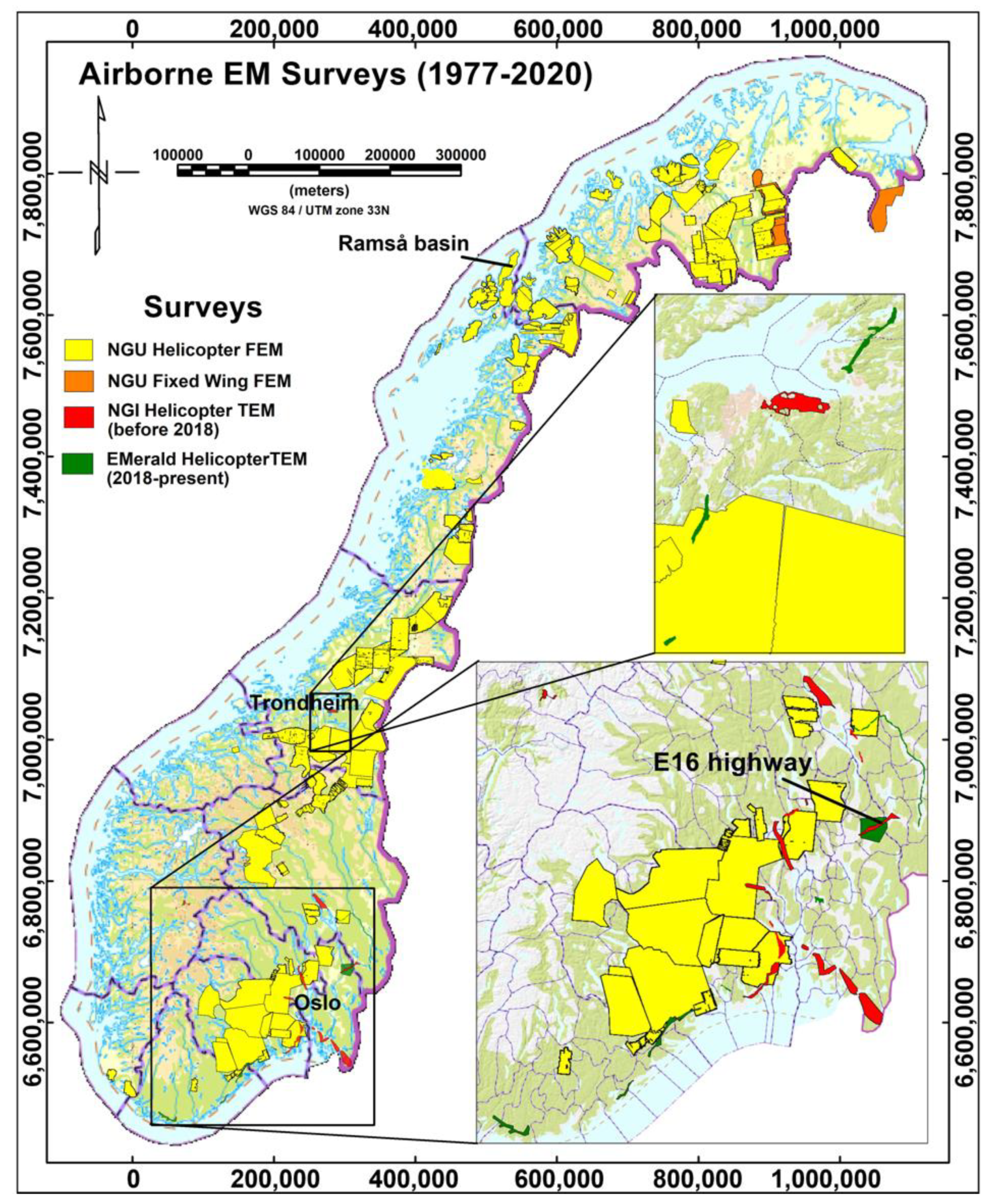
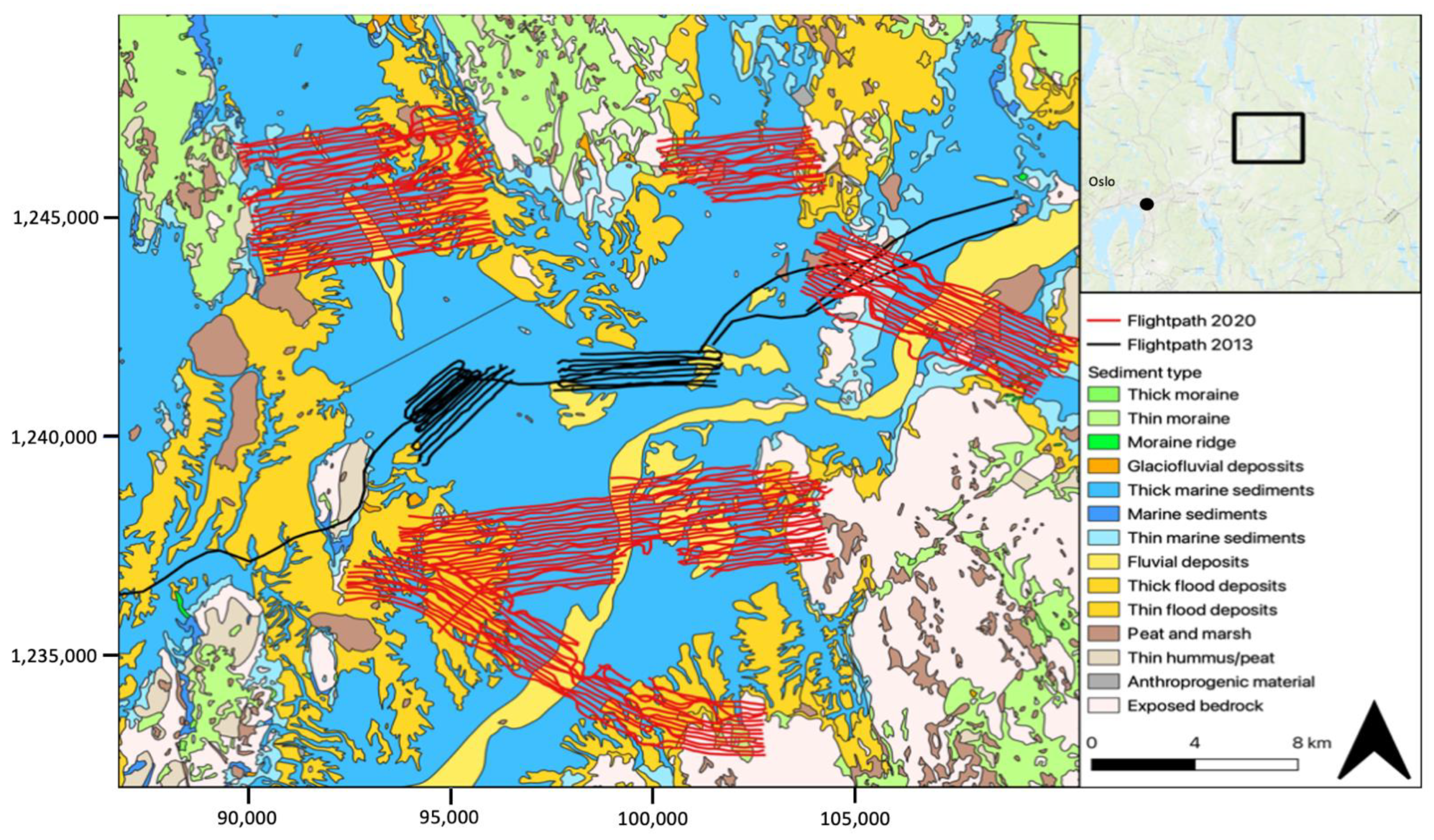
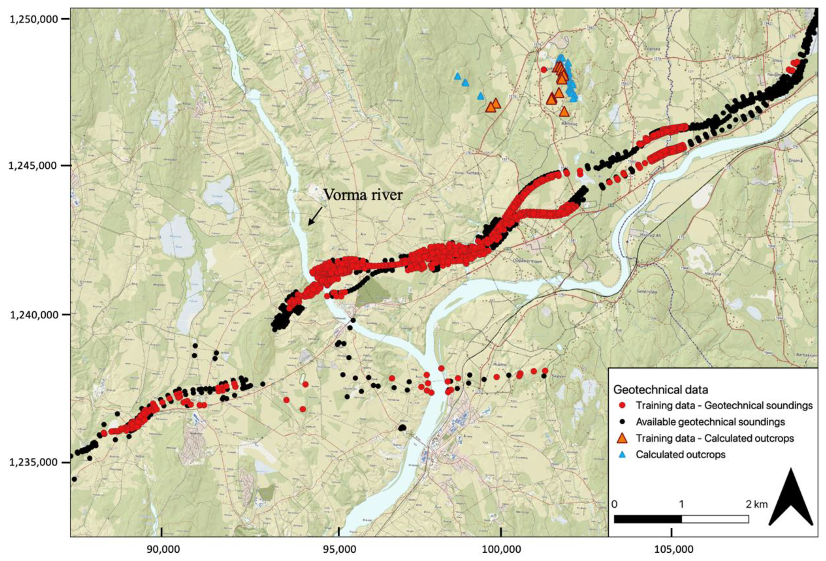
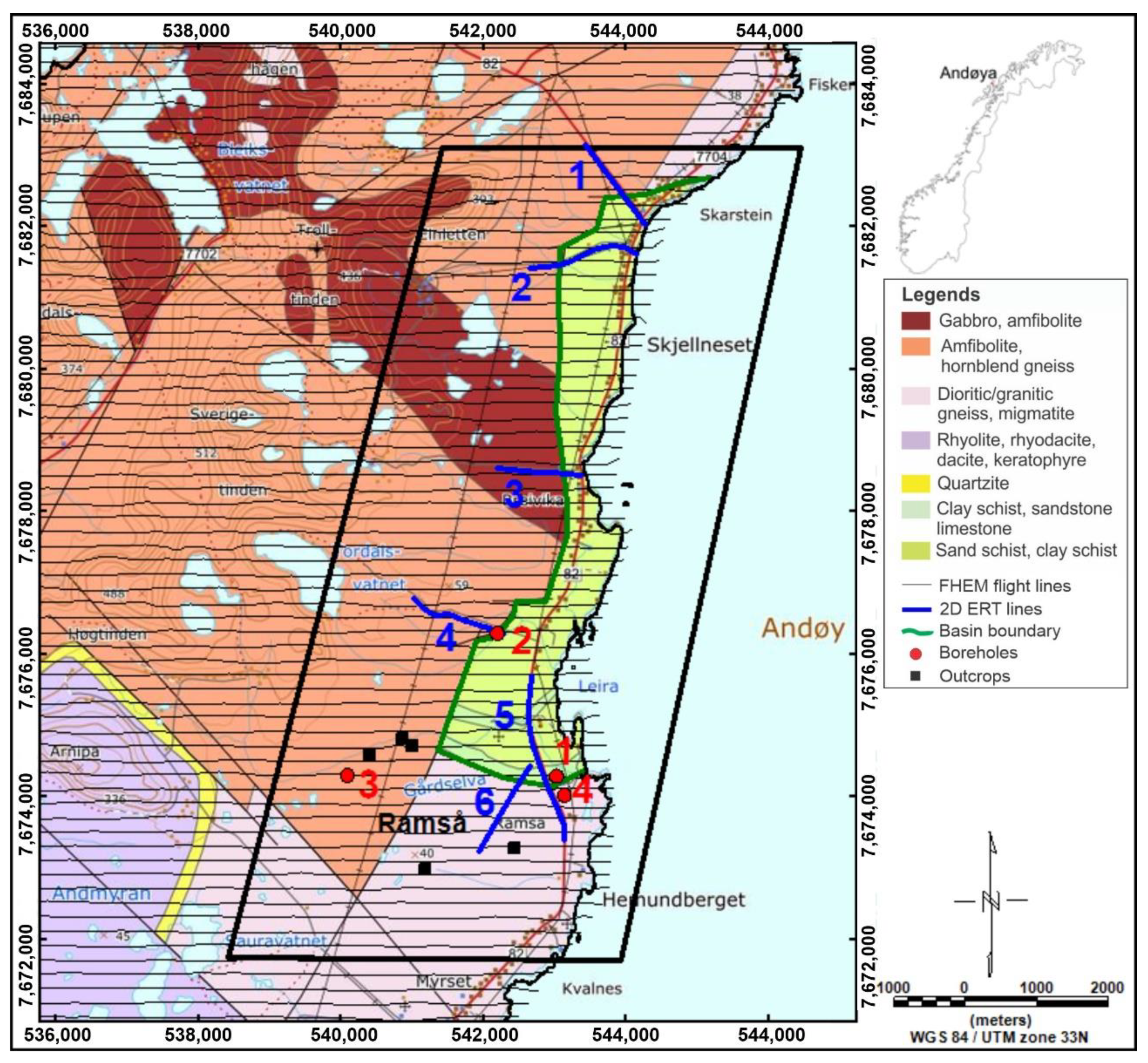
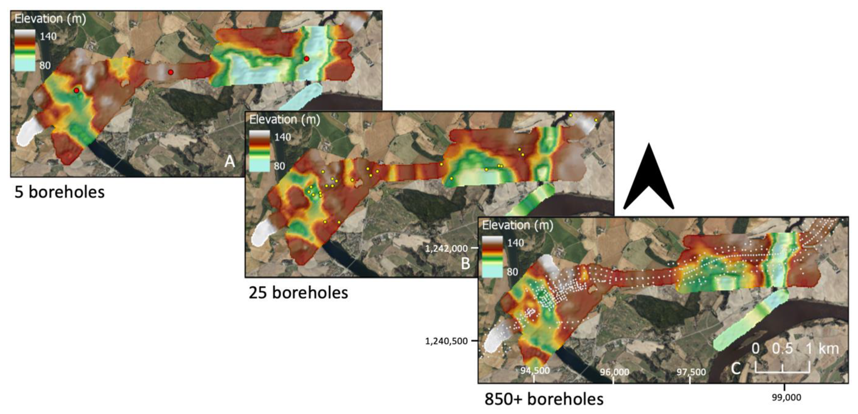
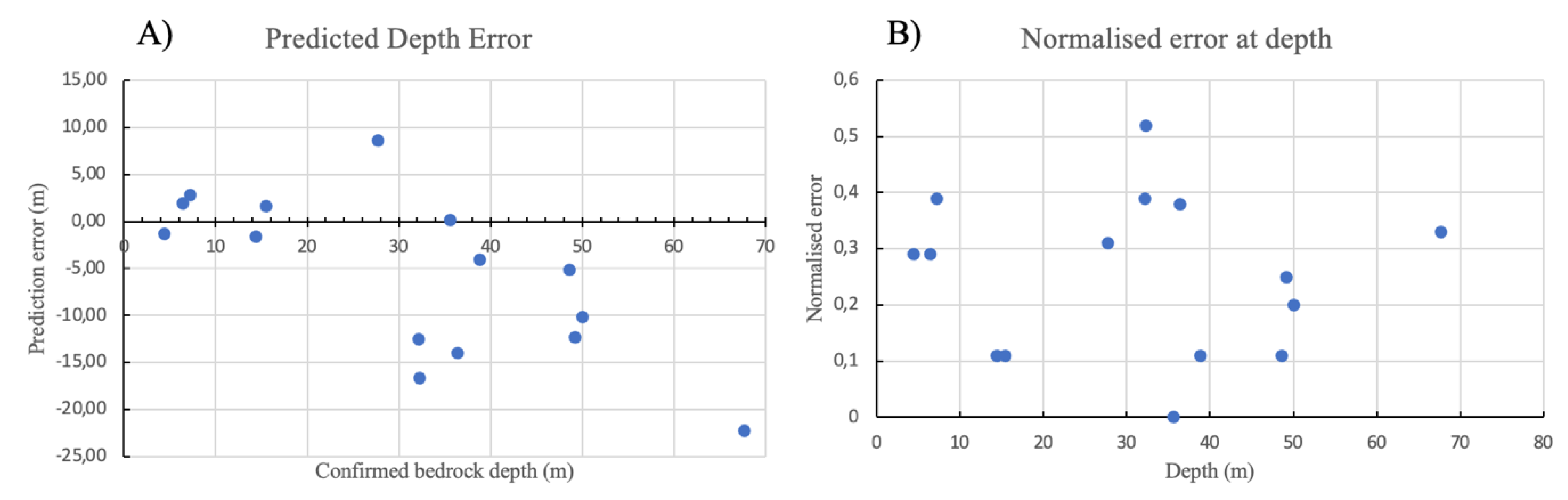
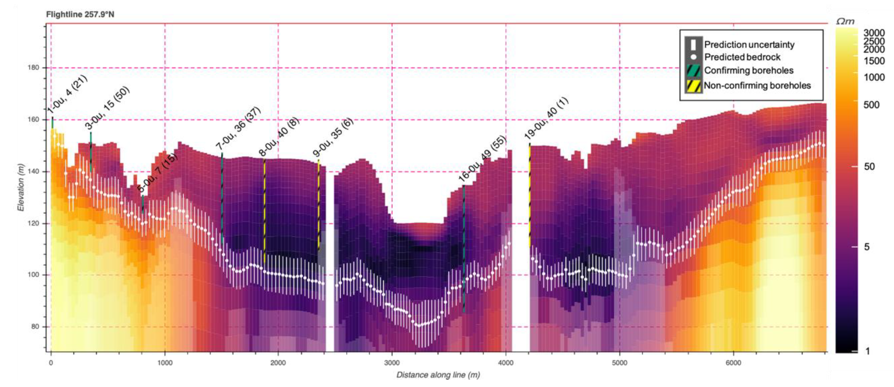

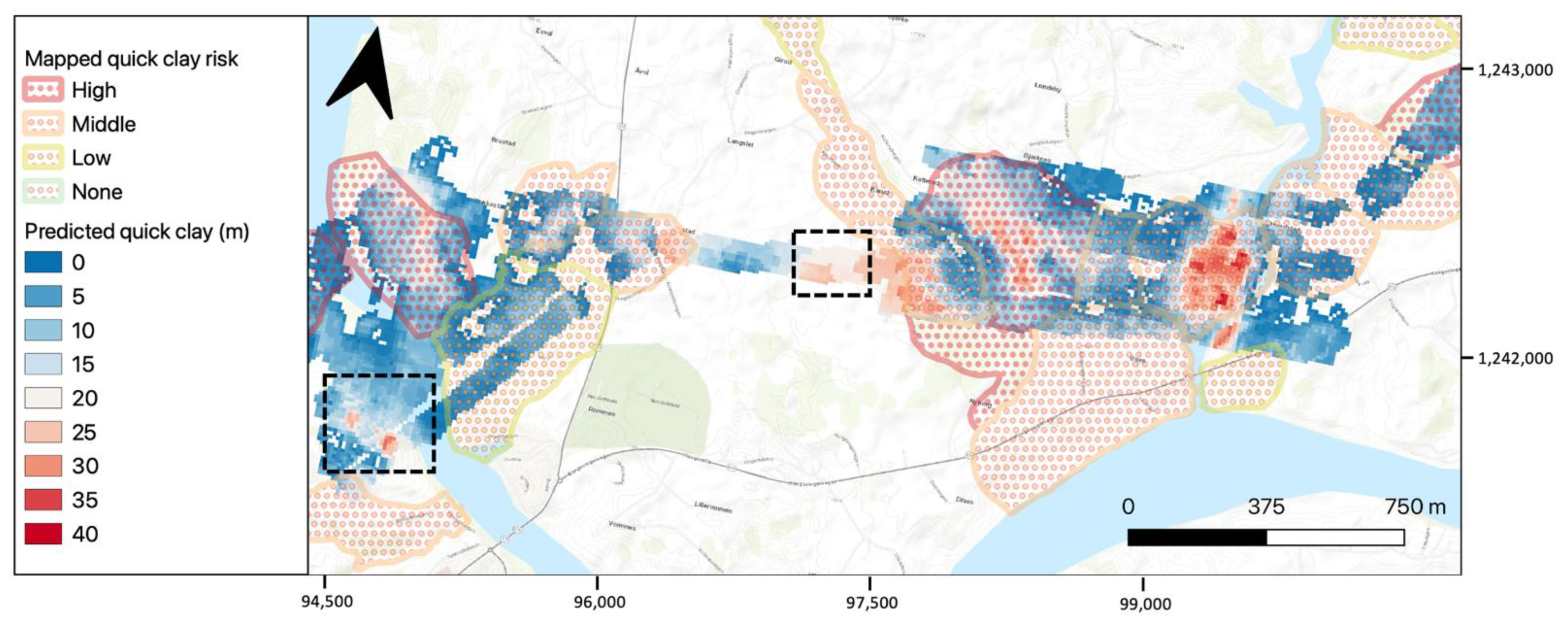
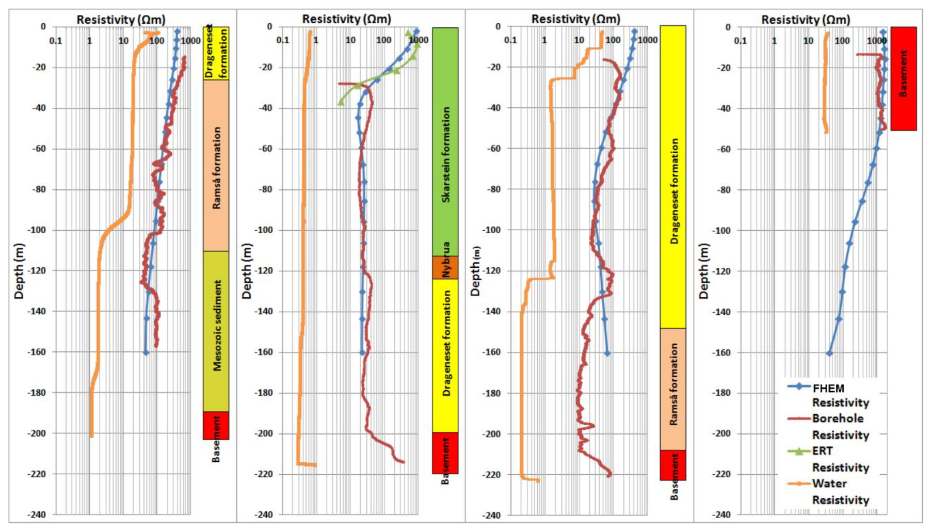
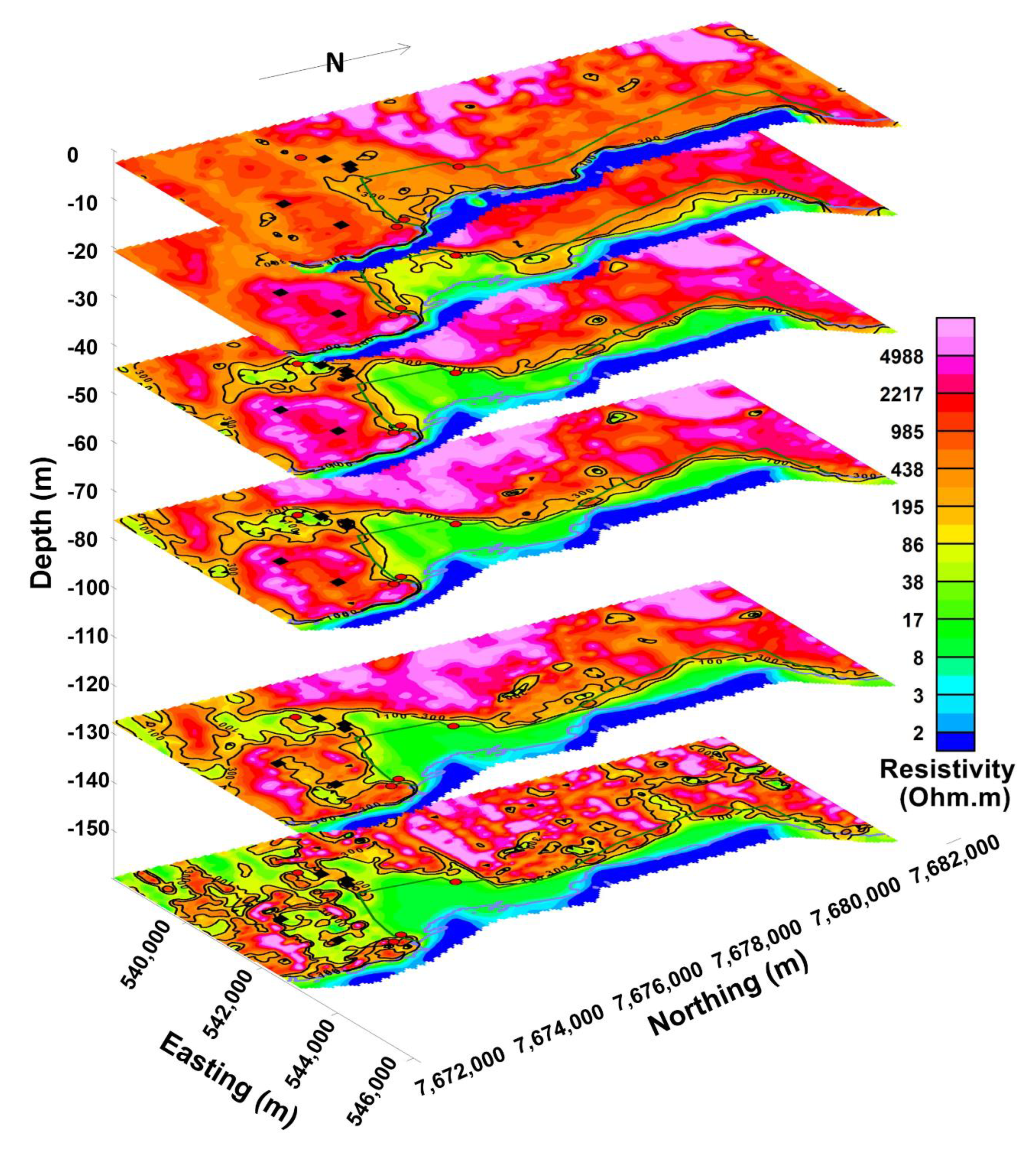
Publisher’s Note: MDPI stays neutral with regard to jurisdictional claims in published maps and institutional affiliations. |
© 2021 by the authors. Licensee MDPI, Basel, Switzerland. This article is an open access article distributed under the terms and conditions of the Creative Commons Attribution (CC BY) license (https://creativecommons.org/licenses/by/4.0/).