Abstract
Satellite Image Time Series (SITS) have been used to build models for predicting Potato (Solanum tuberosum L.) yields at regional scales, but evidence of extension of such models to local field scale for practical use in precision agriculture is lacking. In this study, multispectral data from the Sentinel-2 satellite were used to interpolate continuous spectral signatures of potato canopies and generate vegetation indices and the red edge inflection point (REIP) to relate to marketable yield and stem density. The SITS data were collected from 94 sampling locations across five potato fields in England, United Kingdom. The sampling locations were georeferenced and the number of stems per square meter, as well as marketable yield, were determined at harvest. The first principal components of the temporal variation of each SITS wavelength were extracted and used to generate 54 vegetation indices to relate to the response variables. Marketable yield was negatively related to the overall seasonal reflectance (first principal component) at 559 nm with a beta coefficient of −0.53 (±0.18 at p = 0.05). Seasonal reflectance at 703 nm had a positive significant relationship with Marketable yield. Marketable yield was modeled with a normalized root mean square error (nRMSE) of 0.16 and R2 of 0.65. On the other hand, Stem density was significantly related to the Specific Leaf Area Vegetation Index (β = 1.66 ± 1.59) but the REIP’s farthest position during the season was reached later in dense canopies (β = 1.18 ± 0.79) with a higher reflectance (β = 3.43 ± 1.9). This suggested that denser canopies took longer to reach their maximum chlorophyll intensity and the intensity was lower than in sparse canopies. Potato stem density was modeled with an nRMSE of 0.24 and R2 of 0.51. These results reinforce the importance of SITS analysis as opposed to the use of single-instance intrinsic indices.
1. Introduction
The variation in reflectance of electromagnetic radiation between plants of different species and physiological health conditions has enabled the development of remote sensing applications for crop health monitoring, high throughput phenotyping, and precision agriculture. Satellite-acquired multispectral image data is globally available in the public domain at various temporal intervals from the Landsat series of satellites (up to 30 m resolution, 16 day revisit time) since 1972 [1,2] and the Sentinel satellites (up to 10 m resolution, 5 days revisit time) since 2015 [3]. Satellite image data are often used to derive vegetation indices, most notably the Normalized Difference Vegetation Index (NDVI) developed by [4], which has been widely used for vegetation surface classification and crop health assessments. Since the launch of the Landsat satellite, a highly active research area has emerged to attempting the use of spectral reflectance values of canopies to predict or infer plant-level dependent variables of interest through traditional linear regression models or machine learning approaches. However, while remotely sensed vegetation indices are often well correlated to crop biomass, they often constitute poor indicators of crop yield, which hinders their adoption in yield prediction [5]. Consequently, very little crop-specific published literature exists on the successful use of vegetation indices from satellite image data to model yield attributes. More studies are required to establish methods for robust transformation of remotely sensed spectral reflectance measurements or the different vegetation indices derived from them in order to provide reliable explanatory variables for the crop biomass or yield variables of interest.
The potato is the world’s third most important crop primarily grown for human consumption after wheat and rice [6]. This is partially due to its high ratio of economic biomass to total biomass (harvest index) [7], which is higher than that of all the world’s major cereals (Zea mays, Triticum aestivum, and Oryza sativa) and grain crops [8]. In precision potato agronomy, establishing an accurate estimate of plant density for downstream decision-support is an important open research area due to the complex physiology of the crop. Although planted seed-tuber populations and plant spacing are closely controlled by farmers, potatoes produce highly variable stem numbers per planted tuber and each stem eventually develops its own independent tuber set and acts as an independent plant unit [9]. This makes the number of emerged stems a more representative unit of plant density than using the number of tubers that were planted or the number of plant clusters that emerge from the total planted tuber population. Using the spectral properties of plants, aerial image analysis has been used to predict potato plant density in potatoes [10,11], however, the unit of plant density used in the studies (the number of emerged independent plant clusters per unit area) is not the ideal representative unit of plant population (stem density). While machine learning methods have been used to enumerate potato stems from images collected using unmanned aerial vehicles [12], no previous research has attempted to predict stem density from satellite images. Development of estimation techniques for stem density remains pertinent in potato production, with several studies linking it to tuber size and total yield variations at harvest [9,13,14,15,16].
Studies using satellite imagery for overall yield prediction in advance of harvest are mainly motivated by the need for objective crop production estimates in areas where ground-level records are logistically difficult to acquire [17]. Such predictive models have potentially wide applicability in region-level resource planning and early-warning systems for famine in resource-constrained environments. Therefore, several studies on agricultural yield prediction from satellite imagery have been conducted in semi-arid locations. For example, low resolution (500 m pixel dimensions) satellite imagery from the TERRA MODIS satellite has been used to calculate NDVI and demonstrated ability to explain up to 84% of the variation in potato yield [18]. Predictive models were also developed by [19] based on NDVI and the Soil Adjusted Vegetation Index (SAVI) from 30 m Landsat-8 and 10 m resolution Sentinel-2 satellite images, explaining between 39% and 65% of the variation in potato yield. Additionally, machine learning models have been used to leverage NDVI for the prediction of potato yield, with a large proportion of the variation in yield (up to 86%), accounted for by the empirical models [17]. While these are promising results, the models are based on region-level studies with limited applicability at the farm level and the machine-learning-based models do not provide coefficients that are relatable to biophysical processes. Therefore, opportunity is lost to understand the underpinning phenomena behind the observed relationships for informing future studies. Models designed to infer farm-level phenomena require higher spatial resolution than provided by the MODIS satellite, and there is a general consensus that higher spatial resolution results in better model accuracy [20]. With up to 10 m spatial resolution, the Sentinel-2 satellite, therefore, provides enough detail to model within-field spatial variation in reflectance and potentially infer the processes that affect it. However, In-situ measurements for developing models or validating remotely-sensed reflectance can come at spatial resolutions that are disparate to the satellite product [20,21]. The use of coarse-scale sensors or cropping data to simulate yield neglects fine-scale variability, which raises questions over the usability of such models at finer-resolution than provided by the remote sensor [20]. To resolve this, every pixel of the remote sensing product is typically mapped to a single value of in-situ measurements, which can be determined by appropriate random sampling, or aggregation (resampling) of the in-situ measurements to the resolution of the remote sensing product (See [19,22,23]). While aggregation or collection of a single representative value per pixel allows the combination of in-situ and remotely sensed data, the establishment of relationship coefficients between the two data sources is often biased by the violation of the independence assumption in linear regression modeling, due to spatial autocorrelation [24,25,26]. This remains a significant issue that is often ignored when regression models are produced from remote sensing data, leading to biased coefficient estimates [20,21]. Various statistical modeling techniques including Geographically Weighted Regression [27] have been suggested for unbiased estimation of regression coefficients [20]. Spatial mixed effect modeling techniques [28] provide effective ways of dealing with sample non-independence and they provide for a non-biased integration of clustered data from different study locations to estimate more robust global coefficients. While variations of such approaches are not novel and have been used in remote sensing work (see [29]), evidence of the application of these methods in the context of field-level vegetation cover modeling cannot be readily found in the literature.
The timing of image acquisition and the pre-analysis transformations required of satellite image data are important for the generation of appropriate data from which inferences can be made about the relationship between canopy reflectance and variables of interest. From a physiological standpoint, the final dry matter production in potatoes, from which final marketable yield is derived, is a function of cumulative absorbed radiation throughout the season [30,31]. The final proportion of the daily dry matter that gets allocated to further above-ground vegetative development and/or tuber yield is dependent on a time-varying harvest index [30,32]. Therefore, the temporal rates at which a potato canopy develops, represented by changes in reflectance, are potential indicators of end-of-season yield. Several studies have established the occurrence of an exponential increase towards an asymptotic maximum ground cover and leaf area index in potatoes, followed by an exponential decrease at senescence [30,31,32]. The rate and peak of the exponential functions that describe canopy development are affected by genetic factors (sown variety) [33] and environmental factors such as plant abiotic or biotic stress and plant population [10,34], which all contribute to the final yield. Where the genetic factor is fixed, the rate and asymptotic peak parameters that define the exponential development of the canopy are therefore location-specific and dependent on spatially-variant biotic and abiotic stress factors. Potato crop growth models largely rely on the estimation of temporal absorption of photosynthetically active radiation which exponentially increases to a maxima at full canopy [30], akin to the typical temporal development of NDVI [20]. The subsequent evolution of the harvest index (ratio of economic to total biomass) follows a similar pattern while the total dry matter production follows an exponential growth curve [30,35]. As an implication, a cropping area that maximizes light interception earlier than other parts of the field can be expected to yield more due to relatively more time provided for maximal biomass accumulation in tubers. Therefore, the temporal rate of development of vegetation indices like NDVI can potentially be utilized to predict tuber yield but no studies have empirically evaluated this relationship. Accurate estimation of the peak and rate parameters governing the temporal development of SITS-derived indices is dependent on the regularity of the SITS. Evaluation of the relationship between temporal resolution and model accuracy would require systematic resampling of SITS and different time intervals, which is difficult in cloud-dependent irregular SITS such as those provided by the Sentinel-2 satellite. Several previous studies have used smoothed time series of vegetation indices to extract the index values at each day and correlate to crop yield variables [36,37]. In these previous studies, Pearson’s product-moment correlation was calculated between vegetation indices and yield variables at each day for which valid (cloud-free) satellite imagery was available, then the evolution of the correlation coefficient over time was studied. The day at which the correlation coefficient was maximized was chosen as the optimal day of satellite image collection for the maximum predictive value of yield [36,37]. The main drawback with such methods is that they work best with a high temporal resolution of the satellite imagery over the cropping season, which is not guaranteed in satellite imagery due to erratic cloud cover. Collation of images for the whole season enables better retrospective modeling and good model performance has been reported in previous studies [18,19]. In a time-series study of the relationship between satellite-image-derived NDVI and potato yield, [38] found that the correlation coefficient was highest when NDVI was at its peak, estimated to be at the middle of a typical growing season. Such models offer limited utility for mid-season prediction due to their requirement for full-season data, though the relationship coefficients derived from these studies are important for understanding and deriving hypotheses for the underpinning mechanistic models governing the phenological development of plants with respect to solar radiation absorption. The discovery of effective methods for the extraction of temporal features from irregular SITS and relating them to crop phenology is therefore an open research area for which novelty is required.
The goal of this study was to contribute to the knowledge on the transformations required of Sentinel-2 satellite data to engineer features that can be related to biophysical processes of interest in potatoes. Specifically, the objective of this study was to derive simple temporal peak and rate parameters describing the development of reflectance for selected Sentinel-2 bands and relate them to potato response variables—yield and stem density. The overall temporal development of each band was also encoded as the first principal component and related to the response variables, to infer how end-of-season yield relates to this temporally accumulated variation.
2. Materials and Methods
2.1. Site Characterisation
The study was conducted at five sites as summarized in Table 1. Deaton 6 and HF7 sites were located in marsh-reclaimed land with a shallow water table and high organic matter content. Horse Foxhole, Crabtree Leasow, and Buttery Hill were located in well-drained, slightly stony, sandy loam soil subtended by weathered sandstone. At all the fields, the plow depth during land preparation was 30 cm and beds were formed with 90 cm between rows after destoning. The locations of the fields were as mapped in Figure 1. Within each site, management practices were conducted uniformly across the field throughout the growing period.

Table 1.
Summary of the location and key production information of the study sites.
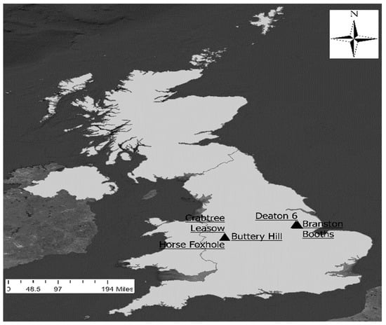
Figure 1.
Map of the United Kingdom territory showing the locations of the 5 study sites (Crabtree Leasow, Horse Foxhole Buttery Hill, Deaton 6, and Branston Booths).
2.2. Sampling Design
To determine representative locations for subsequent yield sampling in each field, a model-based sampling approach was taken. Our sampling was informed using soil color variation as a proxy for the variation of organic matter and by extension soil macronutrient quantities [39,40] that affect yield. The Soil Brightness Index (SBI) as described by [41] was chosen to spatially model the soil color differences at each field. The average SBI for three months prior to crop emergence was calculated using atmospherically corrected (Level-2A) Sentinel-2 satellite imagery of 10 m resolution on manually inspected cloud-free days. From the normalized SBI choropleth map, three zones of relative homogeneity were defined by k-means clustering (k = 3) to define dark-colored soils (k-means cluster centroid ranging from 0.31–0.39), light-colored soils (k-means cluster centroid ranging from 0.78–0.87), and medium hue soils (k-means cluster centroid ranging from 0.56–0.61).
In commercial potato production, the variables of interest of this study (stem density and marketable yield) are likely to only be managed if they exhibit relatively long-range spatial autocorrelation to enable practical mechanized control [42]. It was therefore necessary to define a practical spatial scale for in-situ measurements. In the most recent related large-scale study of the spatial structure of potato stem density and marketable yield in the UK, [42] reported relatively long-range spatial autocorrelation for both stem density (48 m) and marketable yield (114 m). Agricultural yield processes are known to be spatially rough but the decay in spatial autocorrelation is controlled by latent field-scale limiting factors (e.g., variety and soil type) which maintain a long-range logarithmic decay (de Wijs process) rather than an exponential decay process [24,25]. In commercial production, farmers aim to produce uniform plant density across the field and any variation is likely to come from factors such as a systematic fault in the planting operation, low viability of a batch of seed, or soil-borne factors that affect seed germination [43], which have a long-range of autocorrelation relative to the size of the field as observed by [42]. This large-scale autocorrelation in comparison to Sentinel-2 satellite data resolution means that fine-scale in situ data on stem number and yield can be resampled to 10 m or 20 m resolution while maintaining the structure of the spatial variability.
Resampling of sub-pixel-scale in situ data to align with the pixel size of Sentinel-2 data is a common technique deployed previously to model potato yield [19] and other crops [22,23]. During resampling, it is crucial to ensure that the assigned in-situ data are collected with enough locational accuracy such that their true location aligns with a single pixel of the Sentinel-2 data. In-situ sampling resolution must therefore take GPS instrument error into account, in relation to the targeted resampling resolution. In this study, a GarminTM eTrex 20 with 3 m accuracy specification was used to navigate to the yield sampling locations. The aim was to randomly select a sampling point within any 10 m pixel of the SBI map, therefore, a sub-pixel sampling unit of 6 m by 6 m was chosen to ensure that the sampling location was within a single 10 m pixel. A grid of 36 m2 quadrats was imposed across a rasterized SBI surface then random quadrats were then drawn from each stratum as sampling points. An intersection of each drawn sampling point with the 10 m resolution SBI surface was done to check that the drawn sampling point was spatially contained within a single pixel SBI pixel. Statistical power analysis [44] was used to determine the number of sampling points to draw from each stratum to maintain a statistical power of 0.8. The effect size was calculated as the standardized difference between the expected SBI of dark soils and the combined expected SBI of the medium and light clusters. Power analysis was conducted using R [45]. Using ArcGIS [46], the determined sample size was drawn from the grid of 36 m2 quadrats, extracting the centroid pixel from every 6 m by 6 m quadrat. The extracted coordinates were exported into the GarminTM etrex 20 GPS receiver for tracking during yield sampling. Since the GPS receiver had a locational accuracy of 3 m, navigating to the centroid of the 36 m2 quadrat with the maximum possible 3 m offset ensured that the located point was within the intended quadrat.
2.3. Collection and Processing of Satellite Imagery
At each site, all cloud-free dates on which the Sentinel-2 satellite captured data during the growing period were manually inspected. In total, four post-emergence cloud-free images were collected each of five locations (Buttery Hill, Crabtree Leasow, Deaton 6, HF7, and Horse Foxhole). A Keyhole Markup Language (KML) file was created for the spatial extent of each site then the sen2r [47] package in R [45] was used to download 20 m resolution level-2A (atmospherically corrected) tiles covering the spatial extent from the Sentinel-2 image repository at all the determined cloud-free dates, forming SITS. For each retrieved image representing an individual Sentinel-2 band, bicubic interpolation was used to down-sample the raster to 6 m then the sampling points at its corresponding site were superimposed, and the pixel value at which each sampling point fell was extracted and stored. The final raw extracted dataset comprised of a time series of the pixel values of each Sentinel-2 band for each sampling point at the five study sites.
2.4. Principal Component Analysis
For each observation point, each of the nine Sentinel-2 bands (resampled from 20 m to 6 m resolution) had four reflectance measurements taken at four different times during the course of the season. This captured the change in reflectance during the course of the season for each band. In order to create an overall representation of the SITS for the whole season for the observation point, principal component analysis was chosen. Accordingly, at each sampling point, the data was processed by re-arranging the nine bands as observations and the four imaging dates as variables, creating a 9 × 4 matrix. The principal components of the four dates were then computed and the standardized first principal component was determined as a nine-element vector representing the overall temporal variation of the observation. The column vector was then transposed into a row vector with nine variables representing the values of the nine Sentinel-2 bands for the observation. This analysis, therefore, encoded the overall reflectance of each wavelength throughout the season, giving an index for its temporal expression. The percentage of variance explained by the principal component at each observation point was also recorded in order to assess the amount of variation encoded in each component.
2.5. Rates of Change in Reflectance
The daily vegetative growth of a potato plant is a function of intercepted radiation and the radiation use efficiency mediated by the genotype and environment [48]. The intercepted radiation can be estimated as an exponential function of the crop leaf area index (LAI), plateauing at full canopy cover before exponentially decreasing towards senescence [30,38,49]. Previous reports on the temporal profile of spectral reflectance in potatoes, particularly using the Normalized Difference Vegetation Index (NDVI), suggest a similar curve of exponential increase in spectral reflectance towards a maxima followed by an exponential decrease [50,51]. Extracting temporal features of interest in multispectral reflectance like the maximal value and the rate at which the maxima is reached therefore provides proxies for crop growth rates [52]. In this study, at every sampling point, the reflectance at each wavelength was plotted against the days after planting (DAP) on which the satellite imagery was obtained (Figure 2). A second-order polynomial equation was then fitted to the data to model the exponential growth curve towards a peak. The turning point of the polynomial was maximal for wavelengths that are reflected by vegetation (e.g., Near Infrared) as shown in Figure 2, or minimal for wavelengths that are absorbed by vegetation (e.g., water absorption bands).
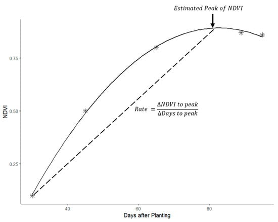
Figure 2.
An illustrative graph showing how spectral index values like the Normalized Difference Vegetation Index (NDVI) were plotted in time and their peak and rate parameters derived.
The reflectance at the turning point of the polynomial was therefore determined as the peak (or trough for absorbed wavelengths) reflectance of the particular wavelength relative to DAP. The rate of growth to maximal reflectance or absorption was calculated by dividing the DAP at the turning point by the reflectance value. Apart from the single wavelengths, several ratio-based vegetation indices were also calculated, as summarized in Table 2. NDVI at tuber initiation was approximated as the NDVI value at 7 weeks after planting.
Table 2.
Summary of the vegetation indices used in the study.
2.6. Estimation of Red-Edge Inflection Points
A basic feature of chloroplast biology, photosystems I and II have their maximum absorption efficiency at 700 nm and 680 nm respectively, beyond which plants exhibit high reflectance of Near Infra-Red (NIR) [56]. This zone of the abrupt shift from absorption to reflection is referred to as the Red Edge [57]. Several studies have shown that reflectance at the red edge inflection point becomes lower and its specific wavelength position shifts higher in vegetation with more chlorophyll-associated absorption of light. Therefore the position of the inflection point and its reflectance is used to model chlorophyll content and hence photosynthetic efficiency as proxies to dry matter accumulation and yield [56,58,59]. The red-edge inflection point can be found by identifying the first derivative of a smoothed spectral profile and finding the position of the peak in the red-edge region [57,60].
In this study, the visible and NIR spectral values derived at each date of sampling were plotted and the Savitzky-Golay filter [61] was used to estimate a smooth spectral signature [52,62]. At each location, the reflectance values of each Sentinel-2 band were extracted, then each cloud-free date’s spectral reflectance signature was plotted as an irregular series. The “sgolay” function from the “Signal” package in the R signal package (v0.7–6) was then used to construct a second-order Savitzky-Golay filter of length 3. The filtered values were used as predictor variables in a linear model to predict the original spectral signature. Prior to fitting the linear model, the filtered and original values were resampled using linear interpolation to produce a value for each wavelength between 492 nm and 864 nm (n = 372). Linear interpolation of Savitzky-Golay filter results to generate continuous series is a common method used in mathematics and computer science [63]. The linear interpolation permitted the fitting of a fifth-order polynomial to allow inflection points at all observed wavelengths and generate smooth curves. The polynomial was fitted as a linear model and the fitted values were used to approximate the continuous spectral signature. The estimated continuous spectral signatures at different time points in the season could then be used to visually evaluate the temporal evolution of the spectral signature.
The first derivative of each smoothed spectral signature was also derived and the wavelength position of the maxima in the red edge was determined and extracted as the red-edge inflection point following [58]. The estimated reflectance at the inflection point was extracted from the smoothed reflectance spectra and this process was repeated for all the dates of cloud-free image availability, then the change in the position of the inflection point during the course of the growing season was examined by plotting the extracted inflection points against DAP. A second-order polynomial was then fitted to the plot and the peak was calculated to extract the most advanced wavelength position of the Red-Edge inflection point (REIP), the DAP of its observation, and the rate of change. The value of the reflectance at the REIP was also extracted (REIPr).
2.7. Yield Data Collection
At every sampling location, a representative one-meter row was randomly demarcated as a yield sampling area. At harvest, the number of plants and main stems within the row was counted and recorded as units of plant density. The number of stems was counted after careful excavation of the one-meter demarcation with a spade to prevent any loss of stems or tubers. In a plant laboratory at Harper Adams University, the number of tubers with a transversal diameter greater than 25 mm at each sampling point was counted then the total weight of tubers was measured to 0.01 g accuracy.
2.8. Statistical Analysis
All tuber yield components were regressed against remotely sensed canopy data to find statistically significant relationships. By design, there were two levels of non-independence in the study. Firstly environmental and management differences between locations meant that observations within a location were more related to each other than those from different locations. Secondly, spatial autocorrelation was expected within a location. Therefore, a spatial mixed-effect model was appropriate for taking the two non-independence factors into account. To minimize assumptions on the autocorrelation structure, a Matérn covariance structure was chosen due to its flexibility in modeling different spatial covariance structures [25,64]. All statistical analyses were conducted in R [45] and the spatial regression modeling was conducted using the SpaMM package [28]. Statistical significance was evaluated using 95% confidence intervals and the goodness of fit for multivariable regressions was evaluated using the Normalized Root Mean Square Error (nRMSE). To calculate the nRMSE, first, the RMSE was calculated as follows:
where N is the number of observations, yi is the predicted value and ýi is the observed value. Then nRMSE was calculated by dividing the RMSE by the mean of the observed value. The coefficient of determination (R2) was computed following [65].
3. Results
3.1. Summary of Spectral Reflectance and Intrinsic Indices
Using a boxplot overlaid with a dot plot, Figure 3 shows the spread of the peak reflectance values of the nine Sentinel-2 wavelengths observed during the growing period at all five study sites. The reflectance pattern of individual wavelengths was typical of the spectral signature of vegetation, showing low reflectance in λ492 and λ665 with higher reflectance in the NIR bands of λ703, λ740, λ780, and λ864. Characteristically, there was higher reflectance of λ559 than λ492 and λ665. At all sites, there was lower variation in the reflectance values of the absorption wavelengths λ492, λ665, λ1610, and λ2186 than the reflected wavelengths. The strong absorption in the photosynthetically active region, coupled with high NIR reflectance confirms that vegetated pixels were effectively sampled in the sampling approach. Furthermore, very little variation was observed in the absorption bands in every field, suggesting relative spatial homogeneity in the absorption of photosynthetically active radiation at the peak of the season in every field. This is expected since only a single variety was planted at every location. However, a larger variation in the NIR band suggested that the slope and location of the red edge varied across a field, a potential indicator of spatially variable vegetation density.
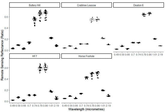
Figure 3.
Illustration of the observed spread of the peak reflectance values of the nine Sentinel-2 wavelengths observed during the growing period at five study sites.
The overall performance of the intrinsic vegetation indices derived from these spectral measurements was as presented in Table 3. The peak NDVI values were close to saturation as is expected for vegetation, the lowest average NDVI being observed at Horse Foxhole (0.81). The gradual temporal increase in NDVI was also apparent, with NDVI at tuber initiation consistently lower than the peak NDVI at all sites. The estimated inflection point ranged from 711 nm at Horse Foxhole to 724 nm at Deaton 6. The peak SLAVI ranged from 3.38 at Horse Foxhole to 5.88 at Deaton 6, suggesting that latent location-specific variables control peak achievable the leaf area index. The standard deviation of the peak NDVI was low, suggesting that late-season NDVI was relatively invariable and a non-ideal indicator of spatial variation at the field scale. More variation was observed in NDVIinit, compared to peak NDVI at all fields, suggesting that the rate of vegetation development was different in a field but the seasonal peak values eventually converge. For modeling yield and stem density as a function of these variables, these results imply that more information about field variability was contained in the temporal rate of growth than the peak values of the intrinsic vegetation indices. Similarly, there was relatively low variation in the furthest reached wavelength of the REIP across the five sites, which suggested a structural constraint to absorption beyond ~725 nm at the maximum canopy. There was however a higher standard deviation in the REIPr, suggesting that the amount of light absorbed at the inflection point—and hence the chlorophyll intensity—was highly variable in a field. These multi-level sources of variation justified the use of a multi-level analysis approach to derive insights on how they related to the final yield and stem density. Indeed, there were location-specific sources of genotypic (variety) and environmental (planting date, season) variation, necessitating a mixed-effects modeling approach to cluster the data by location.
Table 3.
Means and standard deviations (in parentheses) of the peak values of vegetation indices during the potato production season.
As shown in Figure 4, the observed number of days between planting day and the peak value of each intrinsic index was also variable within and between fields. The indices peaked between 90 and 110 days. NDVI peak was observed between 89 days at HF7 and 109 days and Buttery Hill. The farthest wavelength position of the REIP had high variation at Buttery Hill, Crabtree Leasow, and HF7, suggesting considerable spatial variation in the evolution of chlorophyll-related reflectance. Across all sites except Buttery Hill, the highest within-field variation in the number of days to the peak of an index was observed in the REIP, followed by the SLAVI, which are both related to leaf and chlorophyll density. As shown in Figure 5, there was also high within-field variation in the number of days to the maxima (or minima for absorbed wavelengths) of each individual wavelength, ranging from 82 for λ2186 at Horse Foxhole to 130 for λ492 at Buttery Hill. However, there was no discernible and consistent pattern between different wavelengths when either grouped into reflected vs. absorbed wavelengths or sorted in order of wavelength position.
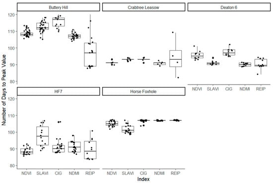
Figure 4.
Illustration of the spread of the observed number of days between planting day and the peak value of Normalized Difference Vegetation Index, Specific Leaf Area Vegetation Index, Normalized Difference Moisture Index, and the Red Edge Inflection Point.
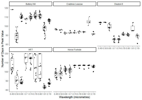
Figure 5.
Illustration of the spread of the observed number of days between planting day and the peak value of each of the Sentinel-2 satellite wavebands.
3.2. Summary of Temporal Variables
3.2.1. Principal Components of Reflectance at Different Time Points
At all five sites, the percentage of variance explained by each of the derived principal components at each observation point were aggregated to assess the amount of total temporal variation encoded in each component. Table 4 shows the percentage of variance explained by the first three principal components averaged at each location. The majority of the variation (>80%) at all locations was explained by the first principal component, with less than 20% of the variance explained by the second component and less than a percentage point by the third component. Since the principal components were fitted on the temporal information at each data point, the consistency of the percentage variation contained in the first principle component shows—as shown by the low standard deviations—that it is a stable index for encoding the temporal variation of each wavelength in a Sentinel-2 pixel.
Table 4.
The mean and standard deviations (in parentheses) of the percentage of variance are explained by the first three principal components of the satellite imagery time series at each sampling point at five locations.
Figure 6 shows the line plot of the standardized first principal component, overlaid with a dot plot of the actual values of the component at all the spectral wavelengths and all locations. The spectral signature of the first principal component was typical of the expected response of vegetation, with strong reflection in the NIR range above 700 nm and strong absorption at λ492 and λ665, including a sharp inflection point around 700 nm. An intermediate level of absorption was observed at λ1610 and λ2186 at Deaton 6, Buttery Hill, Horse Foxhole, and Crabtree Leasow. However, high reflectance in the SWIR was observed at HF7, suggesting overall less moisture available in the canopy throughout the season at this location. This plot shows that the first principle component preserved the information of the spectral signature expected in the crop. Linear modeling of yield and stem density from the first principle component values would therefore have a theoretically relatable interpretation of coefficients.
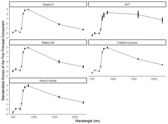
Figure 6.
The spectral signature of the standardized first principal components of each Sentinel-2 waveband’s temporal variation in the potato canopies at 5 different study sites.
3.2.2. Temporal Change in the Spectral Signature and Position of the Red-Edge Inflection Point
Figure 7 shows the monthly change in the average spectral signature for each study site over a three-month period, smoothed using a Savitsky-Golay filter. At all the sites, there was a visual decrease in the reflectance near the Red-edge inflection point with time, most visually discernible at Deaton 6, Horse Foxhole, and Buttery Hill, where the reflectance at ~700 nm was consistently higher in May than June and July. The transition between low reflection ~650 nm and high reflection >700 nm was also sharper in June and July than in May, signifying the development of a sharper red-edge as the crop developed more mature vegetation, reaching full canopy and masking any bare-ground signal. The implication of this was that the position of the inflection point also shifted towards longer wavelengths between the first and second months at all sites, consequent of reduced reflection in the Far-Red region and increased reflection in the NIR region. In the third month, reflection in the NIR decreased at four of five sites (Buttery Hill, Deaton 6, Horse Foxhole, and Crabtree Leasow), possibly due to the onset of canopy senescence. At HF7, the reflectance at the inflection point decreased in the third month coupled with a large increase in NIR reflectance.
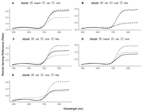
Figure 7.
Smoothed spectral signatures of the potato canopy at the 3 different times of the season at Buttery Hill (A), HF7 (B), Deaton 6 (C), Horse Foxhole (D), and Crabtree Leasow (E).
3.3. Summary Statistics of In-Situ Potato data
Table 5 shows the means and standard deviations of the potato yield components at the five study sites. The marketable yield ranged from 3.32 kg/m2 at Buttery Hill to 5.49 kg/m2 at Horse Foxhole showing large inter-site variation. Within the site, there was also significant variation as evidenced by the large differences in coefficients of variation for each site. Considerable variations were also observed in the number of stems per square meter within a field, ranging from 0.17 Coefficient of Variation (standard deviation divided by the mean) at Deaton 6 and 0.28 Coefficient of Variation at Buttery hill. Overall, Horse Foxhole had the highest stem and plant number due to frequent double-tuber-placement and subsequently recorded the highest yield. The lowest yield was observed at Buttery Hill, which also had very low tuber size and weight compared to the other sites. The between-sites and within-site variations necessitated the use of a mixed model approach with a spatial component to account for spatial autocorrelation when modeling the combinations of satellite-sensed variables in relation to the tuber yield components.
Table 5.
Summary statistics (mean with standard deviation in parentheses) of the potato yield sampling results at five different study sites.
3.4. Linear Model for Marketable Yield
Marketable yield was modeled as a function of the fixed effects λ559, λ703, and CIGpeak, using a spatial mixed-effects structure with the site as a random effect. The fixed effects were chosen based on the theoretical expectation of causation. Table 6 shows the standardized coefficient estimates of the fixed effects as well as their confidence intervals and spatial autocorrelation estimates. Marketable yield significantly decreased with increasing overall reflectance at λ559 (β = −0.53) but increased with increasing overall reflectance at λ703 (β = 0.22). Higher NDVIinit was associated with higher marketable yield, suggesting that higher early-season canopy coverage rates are associated with increased yield. An increase in stem density was also positively associated with marketable yield (β = 0.48). The location random effect structure with a Matérn covariance structure explained 0.27 of the total variance as shown by the intraclass correlation coefficient (ICC1) value, showing that most of the variation in the data was explained by factors other than the random effect structure. As shown in Table 6, the fixed-effect coefficients fitted the data with an nRMSE of 0.16 and the model had an R2 of 0.65.
Table 6.
Estimated coefficients for explanatory variables of marketable yield and the estimated spatial autocorrelation structure.
3.5. Modelling Stem Density
Table 7 shows the standardized coefficient estimates of the fixed effects that best-modeled stem density as well as their confidence intervals and spatial autocorrelation estimates. Stem density was modeled as a function of the peak SLAVI and the rate at which SLAVI was gained before the peak, assuming that areas with lower stem density would gain SLAVI at a higher rate to compensate for the sparse canopy but end up with comparatively lower final SLAVI. It was hypothesized that the shift towards the farthest possible wavelength of the Red Edge inflection point would be slower in higher stem densities due to potentially faster development of leaf area at the expense of chlorophyll intensity. Non-adjusted NDVI before canopy consolidation (NDVIinit) was also used to represent early-season differences in vegetation intensity, which are partly used to model stem and plant density. The Matérn covariance structure was used to account for the spatial autocorrelation at each site. As shown in Table 7, significant positive relationships were observed between stem density and all the variables. Field sections with higher stem densities took longer to reach their maximum possible inflection point and had a higher reflectance at the inflection point. Higher stem density was significantly associated with higher NDVI at tuber initiation (β = 1.19) and a higher SLAVIpeak (β = 1.66), however, the rate of change towards the peak SLAVI was slower at higher stem density data points. These results suggested that dense canopies achieved a higher leaf area index and had higher early-season NDVI but were associated with a delayed date of maximum light absorption per leaf. At the farthest inflection point, denser canopies also absorbed less light (higher reflection). The random effect structure explained 0.28 of the total variance in the stem density. The fixed effect coefficients fitted observed stem densities with nRMSE of 0.34 and the model had an R2 of 0.51.
Table 7.
Estimated coefficients for explanatory variables of potato stem density and the estimated spatial autocorrelation structure.
4. Discussion
The average reflectance of individual Sentinel-2 bands at their peak as shown in Section 3.1 showed a spectral signature typical of vegetation, with high reflectance in the NIR and low reflectance in the visible range [66] at all five locations. The modeling of the temporal change in reflectance from Sentinel-2 SITS as described in Section 2.5, therefore, enabled the derivation of peak spectral signature that was relatable to the typical spectral properties of vegetation. Plotting the first PCA of the SITS on the spectrum space as shown in Section 3.2 also showed high standardized PCA scores in the NIR and low values in the visible range at all five locations. This shows that the dimensionality reduction of the SITS into one variable using PCA still produced variables that are spectrally relatable to the expected reflectance pattern of vegetation. This study showed that most of the temporal variation in the reflectance of individual wavelengths can be represented within the first principal component. This dimensionality reduction enabled the encoding of time information into one dimension while preserving the spectral reflectance information. The high percentage of variation contained within the first principal component compared to the second and third components showed the adequacy of single-dimension decomposition in this case. Subsequent yield modeling also showed that the information in the first principal component was significantly relatable to yield. With temporal information encoded within the principal component, this approach implies that there is potentially no need for conducting correlation analyses on several days of the season in order to find an optimal time of image acquisition for maximizing the correlation between yield and spectral reflectance as implemented in previous studies [36,37]. In forward use cases of this approach, Section 2.4 and Section 2.5 describe the methods needed to replicate the representation of the temporal information. These approaches are replicable where enough cloud-free data is available from the Sentinel-2 repository. In this study, the first principle component was observed to contain the majority of the temporal variation at all 5 sites. While this was consistent across sites, it is still recommended to validate this assumption at any iteration instance and consider the other components, should they hold an equally significant amount of variance.
For the intrinsic indices, the mean NDVI approached saturation at all sites with very little variability within sites, which highlights the limitation of using the indices at full canopy for mapping within-field spatial variation. The observed REIPs between 719.10 nm at Crabtree Leasow and 723.66 nm at Deaton 6 were comparable to previous findings in potatoes using the linearized algebraic formula [67] and observation of first derivative peaks of the reflectance [68]. This adds to the evidence that the REIP falls around 720 nm in potatoes. The temporal pattern, as summarized by the number of days to peak reflectance values as well as the differences in the spectral signatures at different times of the season, shows a rapid early increase in canopy reflectance of NIR (and absorption of visible wavelengths) between May and July, followed by a slight decrease in August, mostly reaching a peak between 90 and 110 days. This implies that an exponential change in ground cover and leaf development leads to an increase in the surface area for NIR reflection towards a peak, which is the growth model expected for potatoes [30]. This observation gives credence to the use of SITS in place of manual canopy assessments for mid-season calibration of potato growth models to map within-field variations.
The multivariable modeling of yield as a function of spectral measurements revealed the significance of the λ559 wavelength in within-field yield modeling. Most studies on the multispectral analysis of the canopy for yield prediction focus on the NDVI, being a well-known index for differentiating vegetation from non-vegetation and quantifying its intensity. This often comes at the expense of the visible wavelengths, especially λ559 which is ignored in most vegetation indices. The analysis showed that high λ559 absorbance was significantly associated with a higher yield, with a high standardized beta coefficient. This suggests that a portion of PAR is absorbed in the green portion of the spectra and contributes significantly to yield. In line with this observation, [66] reported that although plants are highly reflective in the Green portion of the spectrum relative Red and Blue, the Green pigmentation darkens in mature leaves with maximum chlorophyll content, and absorption is observed in the green portion. Mature leaves with maximum chlorophyll content (and therefore relatively high photosynthetic capacity) have lower green reflectance. This is supported by several authors [69,70,71] who report chlorophyll-related absorption in the green wavelengths. Particularly, [70] links high green reflectance to low biomass accumulation in mature wetland vegetation. Furthermore, the high negative coefficients λ559 suggest that areas with a relatively larger reflective surface for λ559 (therefore higher above-ground leaf area) within a field had higher partitioning of photosynthetic products to the canopy at the expense of tubers, in line with the expected widely studied trade-off between canopy and tubers in the development of a harvest index [72,73,74,75]. While reflectance at λ559 is likely to be affected by soil in non-consolidated canopies early in the season, the relative soil effect can be expected to be uniform across the field, assuming relatively consistent soil color. The effect of soil gets diminished over time as potatoes reach maximum ground cover around 50 days after emergence [76]. In this study, the median number of days to peak reflectance of λ559 ranged from 88 at Buttery Hill to 105 at Deaton 6, showing that λ559 intensity continues to develop after the full canopy is reached and the effects of soil are no longer applicable. In line with previous research [9,77], a significant relationship was observed between stem density and marketable yield, showing the relevance of stem density as a unit of plant population with practical relevance for yield modeling. Denser canopies approach full ground cover faster and therefore have a relatively long time of tuber bulking at full canopy hence returning a higher yield potential, which is the basis of many potato yield models [30,78]. In line with this, early-season NDVI—which was used as a proxy to differences in vegetation intensity [17] early in the season at tuber initiation—was observed to positively relate to marketable yield. Reflectance at λ703 and the NIR spectrum portion as a whole is largely associated with the development stage of internal mesophyllic leaf structures that act like reflection and refraction surfaces [66,79]. In this study, the significant positive beta coefficient between overall λ703 reflection and yield is therefore interpreted as a sign of the positive relationship between the surface area available for photosynthesis and the final yield.
The observed positive associations between stem density and the reflectance at the Red-edge inflection point are in line with theoretical expectations of a high reflectance in high stem density (and therefore LAI) canopies due to high NIR scattering [80,81]. Increasing plant density is known to negatively affect chlorophyll content [82] and subsequently higher stem densities are expected to take longer to reach their maximum chlorophyll concentration per plant though there may be higher chlorophyll content on a unit area basis due to more leaves. As observed in the modeled multivariable regression coefficients, high stem densities were significantly associated with higher SLAVIpeak, in agreement with previous research [83]. A lower rate of chlorophyll accumulation per plant in high stem densities [82] means the canopy takes longer to reach its maximum chlorophyll content—and subsequently REIPDAP—as observed in the multivariable model. Finally, Potato stem density is partially a factor of plant density, with higher plant densities resulting in higher stem densities [84]. In previous studies, early-season NDVI has been used to infer plant population from coarse-resolution aerial imagery. In line with our findings from the multivariable modeling, an overall positive relationship between early-season NDVI and plant population density has been reported in several studies [85,86]. These results show that within-field variation in potato stem density can potentially be mapped using SITS, which can be used to map management zones for potential variable harvest timing to optimize tuber size distribution.
5. Conclusions
The temporal profiles of the spectral reflectance of individual bands were revealed to have a significant relationship with potato harvest yield that can be traced to physiological principles related to the spectral properties of plants. In this study, increasing stem density was observed to be related to increases in the position of the REIP and its reflectance value, in agreement with previous studies on the effect of vegetation density on chlorophyll intensity and the REIP. Additionally, increasing stem density was associated with higher NDVI values early in the season (at tuber initiation), showing that intrinsic vegetation indices derived from the Sentinel-2 satellite data can be related to this response variable. Some Sentinel-2 data-based indicators of marketable yield were also discovered in this study. Early-season NDVI was significantly related to marketable yield, as were temporally aggregated reflectance at λ559 and λ703, aggregated as the first principle components of the temporal variation. This study reinforces the validity of SITS analysis as an alternative to the use of single-instance values of vegetation indices like the peak NDVI. The λ559 band is seldom reported in spectral analysis, but this study shows that temporal change during the growing season can be predictive of yield. This study, therefore, draws attention to λ559, an often discounted spectral band due to ubiquitous reliance on intrinsic indices like the NDVI that favor modeling the larger-scale difference between NIR reflectance and Red than Green wavelengths. The complex nature of yield processes requires the use of multivariable modeling and temporal feature engineering, which was shown in this study to yield useful models and highlight significant temporal variables. Finally, this study shows that potato main stem density variation can be modeled from temporal features engineered from SITS with a low RMSE when the spatial covariance of stem density is taken into account. In line with the objectives, emphasis must be made that the models developed in the study are inferential and meant to enhance current understanding of the relationships between reflectance signals picked up by the Sentinel-2 satellite and the observed ground-truth while controlling for within-field spatial effects and clustering of data in multiple locations. The coefficients generated in these models take into account the site-specific spatial covariance structure fitted using the Matérn function at the five sites. Therefore, the coefficients are valid within the confines of the study’s data generating processes, though the significance of the coefficients in the context of the proposed physiological links point to the presence of key relationships that must inform future studies and/or feature engineering for predictive models.
Author Contributions
Conceptualization, J.K.M.; methodology, J.K.M., J.M.M., W.E.H. and J.K.M.; validation, J.K.M., W.E.H. and J.K.M.; investigation, J.M.M. and J.K.M.; resources, J.M.M.; data curation, J.K.M.; writing—original draft preparation, J.K.M.; writing—review and editing, J.K.M., J.M.M. and W.E.H.; visualization, J.K.M.; supervision, J.M.M. and W.E.H.; project administration, J.M.M.; funding acquisition, J.M.M. All authors have read and agreed to the published version of the manuscript.
Funding
This research was funded by the Agriculture and Horticulture Development Board, Stoneleigh Park, Kenilworth, Warwickshire, CV8 2TL, United Kingdom Project Number 11140054.
Institutional Review Board Statement
Not applicable.
Informed Consent Statement
Not applicable.
Data Availability Statement
The data presented in this study are available on request to the corresponding author.
Acknowledgments
Acknowledgement to the Crops and Environment Research Centre of Harper Adams University (TF10 8NB, Edgmond, Shropshire, United Kingdom) and the Agriculture and Horticulture Development Board’s Potatoes Division (Sutton Bridge, Spalding, Lincolnshire, PE12 9YD, United Kingdom) for providing the experimental sites and for this study.
Conflicts of Interest
The authors declare no conflict of interest.
References
- Dev Acharya, T.; Yang, I. Exploring landsat 8. Int. J. IT Eng. Appl. Sci. Res. 2015, 4, 4–10. [Google Scholar]
- Bauer, M.E. Identification of agricultural crops by computer processing of ERTS-MSS data. LARS Tech. Reports Pap. 1973, 20, 1–9. [Google Scholar]
- Szantoi, Z.; Strobl, P. Copernicus sentinel-2 calibration and validation. Eur. J. Remote. Sens. 2019, 52, 253–255. [Google Scholar] [CrossRef]
- Rouse, J.W.; Haas, R.H.; Schell, J.A.; Deeering, D. Monitoring vegetation systems in the Great Plains with ERTS (Earth Resources Technology Satellite). NASA Spec. Publ. 1974, 351, 309. [Google Scholar]
- Turvey, C.G.; McLaurin, M.K. Applicability of the normalized difference vegetation index (NDVI) In index-based crop insurance design. Weather. Clim. Soc. 2012, 4, 271–284. [Google Scholar] [CrossRef]
- De Jong, H. Impact of the potato on society. Am. J. Potato Res. 2016, 93, 415–429. [Google Scholar] [CrossRef]
- Bradshaw, J.E.; Ramsay, G. Potato origin and production. In Advances in Potato Chemistry and Technology; Academic Press: Cambridge, MA, USA, 2009; pp. 1–26. [Google Scholar] [CrossRef]
- Unkovich, M.; Baldock, J.; Forbes, M. Variability in harvest index of grain crops and potential significance for carbon accounting: Examples from australian agriculture. Adv. Agron. 2010, 105, 173–219. [Google Scholar] [CrossRef]
- Knowles, N.R.; Knowles, L.O. Manipulating stem number, tuber set, and yield relationships for northern- and southern-grown potato seed lots. Crop. Sci. 2006, 46, 284–296. [Google Scholar] [CrossRef]
- Li, B.; Xu, X.; Han, J.; Zhang, L.; Bian, C.; Jin, L.; Liu, J. The estimation of crop emergence in potatoes by UAV RGB imagery. Plant Methods 2019, 15, 15. [Google Scholar] [CrossRef]
- Mhango, J.K.; Harris, E.W.; Green, R.; Monaghan, J.M. Mapping potato plant density variation using aerial imagery and deep learning techniques for precision agriculture. Remote Sens. 2021, 13, 2705. [Google Scholar] [CrossRef]
- Mhango, J.K.; Grove, I.G.; Hartley, W.; Harris, E.W.; Monaghan, J.M. Applying colour-based feature extraction and transfer learning to develop a high throughput inference system for potato (Solanum tuberosum L.) stems with images from unmanned aerial vehicles after canopy consolidation. Precis. Agric. 2021. Published online. [Google Scholar] [CrossRef]
- Bleasdale, J.K.A. Relationships between set characters and yield in maincrop potatoes. J. Agric. Sci. 1965, 64, 361–366. [Google Scholar] [CrossRef]
- Gray, D. Spacing and harvest date experiments with Maris Peer potatoes. J. Agric. Sci. 1972, 79, 281–290. [Google Scholar] [CrossRef]
- Love, S.L.; Thompson-Johns, A. Seed piece spacing influences yield, tuber size distribution, stem and tuber density, and net returns of three processing potato cultivars. HortScience 1999, 34, 629–633. [Google Scholar] [CrossRef]
- Wurr, D.C.E. Some effects of seed size and spacing on the yield and grading of two maincrop potato varieties: I. Final yield and its relationship to plant population. J. Agric. Sci. 1974, 82, 37–45. [Google Scholar] [CrossRef]
- Salvador, P.; Gómez, D.; Sanz, J.; Casanova, J.L. Estimation of potato yield using satellite data at a municipal level: A machine learning approach. ISPRS Int. J. Geo Inf. 2020, 9, 343. [Google Scholar] [CrossRef]
- Bala, S.K.; Islam, A.S. Correlation between potato yield and MODIS-derived vegetation indices. Int. J. Remote Sens. 2009, 30, 2491–2507. [Google Scholar] [CrossRef]
- Al-Gaadi, K.A.; Hassaballa, A.A.; Tola, E.; Kayad, A.G.; Madugundu, R.; Alblewi, B.; Assiri, F. Prediction of potato crop yield using precision agriculture techniques. PLoS ONE 2016, 11, e0162219. [Google Scholar] [CrossRef] [PubMed]
- Kharel, T.P.; Ashworth, A.J.; Owens, P.R.; Buser, M. Spatially and temporally disparate data in systems agriculture: Issues and prospective solutions. Agron. J. 2020, 112, 4498–4510. [Google Scholar] [CrossRef]
- Ali, I.; Cawkwell, F.; Dwyer, E.; Barrett, B.; Green, S. Satellite remote sensing of grasslands: From observation to management. J. Plant Ecol. 2016, 9, 649–671. [Google Scholar] [CrossRef]
- Hunt, M.L.; Blackburn, G.A.; Carrasco, L.; Redhead, J.W.; Rowland, C.S. High resolution wheat yield mapping using Sentinel-2. Remote Sens. Environ. 2019, 233, 111410. [Google Scholar] [CrossRef]
- Escolà, A.; Badia, N.; Arnó, J.; Martínez-Casasnovas, J.A. Using Sentinel-2 images to implement Precision Agriculture techniques in large arable fields: First results of a case study. Adv. Anim. Biosci. 2017, 8, 377–382. [Google Scholar] [CrossRef]
- McCullagh, P.; Clifford, D. Evidence for conformal invariance of crop yields. Proc. R. Soc. A Math. Phys. Eng. Sci. 2006, 462, 2119–2143. [Google Scholar] [CrossRef]
- Minasny, B.; McBratney, A.B. The Matérn function as a general model for soil variograms. Geoderma 2005, 128, 192–207. [Google Scholar] [CrossRef]
- Minasny, B.; McBratney, A.B. A conditioned Latin hypercube method for sampling in the presence of ancillary information. Comput. Geosci. 2006, 32, 1378–1388. [Google Scholar] [CrossRef]
- O’sullivan, D. Geographically Weighted Regression: The Analysis of Spatially Varying Relationships; John Wiley & Sons: Hoboken, NJ, USA, 2003. [Google Scholar] [CrossRef]
- Rousset, F.; Ferdy, J.B. Testing environmental and genetic effects in the presence of spatial autocorrelation. Ecography 2014, 37, 781–790. [Google Scholar] [CrossRef]
- Unnithan, S.L.K.; Gnanappazham, L. Spatiotemporal mixed effects modeling for the estimation of PM 2.5 from MODIS AOD over the Indian subcontinent. GIScience Remote. Sens. 2020, 57, 159–173. [Google Scholar] [CrossRef]
- Kooman, P.L.; Haverkort, A.J. Modelling development and growth of the potato crop influenced by temperature and daylength: LINTUL-POTATO. In Potato Ecology and Modelling of Crops under Conditions Limiting Growth; Springer: Dordrecht, The Netherlands, 1995; pp. 41–59. [Google Scholar] [CrossRef]
- Silva-Díaz, C.; Ramírez, D.A.; Rinza, J.; Ninanya, J.; Loayza, H.; Gómez, R.; Anglin, N.L.; Eyzaguirre, R.; Quiroz, R. Radiation interception, conversion and partitioning efficiency in potato landraces: How far are we from the optimum? Plants 2020, 9, 787. [Google Scholar] [CrossRef]
- Haverkort, A.J.; Franke, A.C.; Steyn, J.M.; Pronk, A.A.; Caldiz, D.O.; Kooman, P.L. A robust potato model: LINTUL-POTATO-DSS. Potato Res. 2015, 58, 313–327. [Google Scholar] [CrossRef]
- Geremew, E.B.; Steyn, J.M.; Annandale, J.G. Evaluation of growth performance and dry matter partitioning of four processing potato (Solanum tuberosum) cultivars. New Zealand J. Crop. Hortic. Sci. 2007, 35, 385–393. [Google Scholar] [CrossRef]
- Machefer, M.; Lemarchand, F.; Bonnefond, V.; Hitchins, A.; Sidiropoulos, P. Mask R-CNN refitting strategy for plant counting and sizing in UAV imagery. Remote Sens. 2020, 12, 3015. [Google Scholar] [CrossRef]
- Goudriaan, J.; Monteith, J.L. A mathematical function for crop growth based on light interception and leaf area expansion. Ann. Bot. 1990, 66, 695–701. [Google Scholar] [CrossRef]
- Thapa, S.; Rudd, J.C.; Xue, Q.; Bhandari, M.; Reddy, S.K.; Jessup, K.E.; Liu, S.; Devkota, R.N.; Baker, J.; Baker, S. Use of NDVI for characterizing winter wheat response to water stress in a semi-arid environment. J. Crop. Improv. 2019, 33, 633–648. [Google Scholar] [CrossRef]
- Aparicio, N.; Villegas, D.; Casadesus, J.; Araus, J.L.; Royo, C. Spectral vegetation indices as nondestructive tools for determining durum wheat yield. Agron. J. 2000, 92, 83–91. [Google Scholar] [CrossRef]
- Johnson, D.M. A comprehensive assessment of the correlations between field crop yields and commonly used MODIS products. Int. J. Appl. Earth Obs. Geoinf. 2016, 52, 65–81. [Google Scholar] [CrossRef]
- Yang, Y.; Luo, Y.; Lu, M.; Schädel, C.; Han, W. Terrestrial C:N stoichiometry in response to elevated CO2 and N addition: A synthesis of two meta-analyses. Plant Soil 2011, 343, 393–400. [Google Scholar] [CrossRef]
- Costa, J.J.F.; Giasson, É.; da Silva, E.B.; Coblinski, J.A.; Tiecher, T. Use of color parameters in the grouping of soil samples produces more accurate predictions of soil texture and soil organic carbon. Comput. Electron. Agric. 2020, 177, 105710. [Google Scholar] [CrossRef]
- Mponela, P.; Snapp, S.; Villamor, G.B.; Tamene, L.; Le, Q.B.; Borgemeister, C. Digital soil mapping of nitrogen, phosphorus, potassium, organic carbon and their crop response thresholds in smallholder managed escarpments of Malawi. Appl. Geogr. 2020, 124, 102299. [Google Scholar] [CrossRef]
- Taylor, J.A.; Chen, H.; Smallwood, M.; Marshall, B. Investigations into the opportunity for spatial management of the quality and quantity of production in UK potato systems. Field Crop. Res. 2018, 229, 95–102. [Google Scholar] [CrossRef]
- Bohl, W.H.; Stark, J.C.; McIntosh, C.S. Potato seed piece size, spacing, and seeding rate effects on yield, quality and economic return. Am. J. Potato Res. 2011, 88, 470–478. [Google Scholar] [CrossRef]
- Cohen, J. Statistical Power for the Social Sciences; Laurence Erlbaum Assoc: Hillsdale, NJ, USA, 1988. [Google Scholar]
- R. Core Team. R: A Language and Environment for Statistical Computing; R Foundation for Statistical Computing: Vienna, Austria, 2019. [Google Scholar]
- ESRI. ArcGIS Pro (Version 2.5.2); Environmental Systems Research Institute: West Redlands, CA, USA, 2020; Available online: https://www.esri.com/en-us/arcgis/products/arcgis-pro/overview (accessed on 22 September 2020).
- Ranghetti, L.; Boschetti, M.; Nutini, F.; Busetto, L. “sen2r”: An R toolbox for automatically downloading and preprocessing Sentinel-2 satellite data. Comput. Geosci. 2020, 139, 104473. [Google Scholar] [CrossRef]
- Wolf, J. Comparison of two potato simulation models under climate change. I. Model calibration and sensitivity analyses. Clim. Res. 2002, 21, 173–186. [Google Scholar] [CrossRef]
- Wolf, J.; Van Oijen, M. Modelling the dependence of European potato yields on changes in climate and CO2. Agric. For. Meteorol. 2002, 112, 217–231. [Google Scholar] [CrossRef]
- Shamal, S.A.M.; Weatherhead, K. Assessing spectral similarities between rainfed and irrigated croplands in a humid environment for irrigated land mapping. Outlook Agric. 2014, 43, 109–114. [Google Scholar] [CrossRef]
- Islam, A.S.; Bala, S.K. Assessment of potato phenological characteristics using MODIS-derived NDVI and LAI information. GIScience Remote Sens. 2008, 45, 454–470. [Google Scholar] [CrossRef]
- Velichkova, K.; Krezhova, D. Extraction of the red edge position from hyperspectral reflectance data for plant stress monitoring. In AIP Conference Proceedings; AIP Publishing LLC: Melville, NY, USA, 2019; p. 130018. [Google Scholar] [CrossRef]
- Lymburner, L.; Beggs, P.J.; Jacobson, C.R. Estimation of canopy-average surface-specific leaf area using Landsat TM data. Photogramm. Eng. Remote. Sens. 2000, 66, 183–191. [Google Scholar]
- Gitelson, A.A.; Viña, A.; Arkebauer, T.J.; Rundquist, D.C.; Keydan, G.; Leavitt, B. Remote estimation of leaf area index and green leaf biomass in maize canopies. Geophys. Res. Lett. 2003, 30. [Google Scholar] [CrossRef]
- Wilson, E.H.; Sader, S.A. Detection of forest harvest type using multiple dates of Landsat TM imagery. Remote Sens. Environ. 2002, 80, 385–396. [Google Scholar] [CrossRef]
- Hallik, L.; Kuusk, A.; Lang, M.; Kuusk, J. Reflectance properties of hemiboreal mixed forest canopies with focus on red edge and near infrared spectral regions. Remote Sens. 2019, 11, 1717. [Google Scholar] [CrossRef]
- Horler, D.N.H.; Dockray, M.; Barber, J. The red edge of plant leaf reflectance. Int. J. Remote Sens. 1983, 4, 273–288. [Google Scholar] [CrossRef]
- Gitelson, A.A.; Merzlyak, M.N.; Lichtenthaler, H.K. Detection of red edge position and chlorophyll content by reflectance measurements near 700 nm. J. Plant Physiol. 1996, 148, 501–508. [Google Scholar] [CrossRef]
- Vogelmann, J.E.; Rock, B.N.; Moss, D.M. Red edge spectral measurements from sugar maple leaves. Int. J. Remote Sens. 1993, 14, 1563–1575. [Google Scholar] [CrossRef]
- Smith, K.L.; Steven, M.D.; Colls, J.J. Use of hyperspectral derivative ratios in the red-edge region to identify plant stress responses to gas leaks. Remote Sens. Environ. 2004, 92, 207–217. [Google Scholar] [CrossRef]
- Savitzky, A.; Golay, M.J.E. Smoothing and differentiation of data by simplified least squares procedures. Anal. Chem. 1964, 36, 1627–1639. [Google Scholar] [CrossRef]
- Ishikawa, D.; Hoogenboom, G.; Hakoyama, S.; Ishiguro, E. A potential of the growth stage estimation for paddy rice by using chlorophyll absorption bands in the 400-1100 nm region. J. Agric. Meteorol. 2015, 71, 24–31. [Google Scholar] [CrossRef]
- Pan, Z.; Hu, Y.; Cao, B. Construction of smooth daily remote sensing time series data: A higher spatiotemporal resolution perspective. Open Geospat. Data Softw. Stand. 2017, 2, 25. [Google Scholar] [CrossRef][Green Version]
- Stein, M.L. Interpolation of Spatial Data; Springer: New York, NY, USA, 1999. [Google Scholar] [CrossRef]
- Nakagawa, S.; Johnson, P.C.D.; Schielzeth, H. The coefficient of determination R 2 and intra-class correlation coefficient from generalized linear mixed-effects models revisited and expanded. J. R. Soc. Interface 2017, 14, 20170213. [Google Scholar] [CrossRef] [PubMed]
- Gates, D.M.; Keegan, H.J.; Schleter, J.C.; Weidner, V.R. Spectral properties of plants. Appl. Opt. 1965, 4, 11–20. [Google Scholar] [CrossRef]
- Herrmann, I.; Pimstein, A.; Karnieli, A.; Cohen, Y.; Alchanatis, V.; Bonfil, D.J. LAI assessment of wheat and potato crops by VENμS and Sentinel-2 bands. Remote Sens. Environ. 2011, 115, 2141–2151. [Google Scholar] [CrossRef]
- Fernández, C.I.; Leblon, B.; Haddadi, A.; Wang, K.; Wang, J. Potato late blight detection at the leaf and canopy levels based in the red and red-edge spectral regions. Remote Sens. 2020, 12, 1292. [Google Scholar] [CrossRef]
- Datt, B. Remote sensing of chlorophyll a, chlorophyll b, chlorophyll a+b, and total carotenoid content in eucalyptus leaves. Remote Sens. Environ. 1998, 66, 111–121. [Google Scholar] [CrossRef]
- Lorenzen, B.; Jensen, A. Reflectance of blue, green, red and near infrared radiation from wetland vegetation used in a model discriminating live and dead above ground biomass. New Phytol. 1988, 108, 345–355. [Google Scholar] [CrossRef]
- Sims, D.A.; Gamon, J.A. Relationships between leaf pigment content and spectral reflectance across a wide range of species, leaf structures and developmental stages. Remote Sens. Environ. 2002, 81, 337–354. [Google Scholar] [CrossRef]
- Bélanger, G.; Walsh, J.R.; Richards, J.E.; Milbum, P.H.; Ziadi, N. Tuber growth and biomass partitioning of two potato cultivars grown under different n fertilization rates with and without irrigation. Am. J. Potato Res. 2001, 78, 109–117. [Google Scholar] [CrossRef]
- Mackerron, D.K.L.; Heilbronn, T.D. A method for estimating harvest indices for use in surveys of potato crops. Potato Res. 1985, 28, 279–282. [Google Scholar] [CrossRef]
- Oparka, K.J. Changes in partitioning of current assimilate during tuber bulking in potato (solarium tuberosum l.) cv maris piper. Ann. Bot. 1985, 55, 705–713. [Google Scholar] [CrossRef]
- Oparka, K.J.; Davies, H.V.; Prior, D.A.M. The influence of applied nitrogen on export and partitioning of current assimilate by field-grown potato plants. Ann. Bot. 1987, 59, 311–323. [Google Scholar] [CrossRef]
- Connell, T.R.; Binning, L.K.; Schmitt, W.G. A canopy development model for potatoes. Am. J. Potato Res. 1999, 76, 153–159. [Google Scholar] [CrossRef]
- O’Brien, P.J.; Allen, E.J. Effects of seed crop husbandry, seed source, seed tuber weight and seed rate on the growth of ware potato crops. J. Agric. Sci. 1992, 119, 355–366. [Google Scholar] [CrossRef]
- Aliche, E.B.; Oortwijn, M.; Theeuwen, T.P.J.M.; Bachem, C.W.B.; Visser, R.G.F.; van der Linden, C.G. Drought response in field grown potatoes and the interactions between canopy growth and yield. Agric. Water Manag. 2018, 206, 20–30. [Google Scholar] [CrossRef]
- Knipling, E.B. Physical and physiological basis for the reflectance of visible and near-infrared radiation from vegetation. Remote Sens. Environ. 1970, 1, 155–159. [Google Scholar] [CrossRef]
- Kamenova, I.; Dimitrov, P. Evaluation of Sentinel-2 vegetation indices for prediction of LAI, fAPAR and fCover of winter wheat in Bulgaria. Eur. J. Remote Sens. 2020, 54 (Suppl. 1), 89–108. [Google Scholar] [CrossRef]
- Clevers, J.; Kooistra, L.; van den Brande, M. Using Sentinel-2 Data for Retrieving LAI and Leaf and Canopy Chlorophyll Content of a Potato Crop. Remote Sens. 2017, 9, 405. [Google Scholar] [CrossRef]
- Rietra, R.P.J.J.; Heinen, M.; Dimkpa, C.O.; Bindraban, P.S. Effects of nutrient antagonism and synergism on yield and fertilizer use efficiency. Commun. Soil Sci. Plant Anal. 2017, 48, 1895–1920. [Google Scholar] [CrossRef]
- Chapepa, B.; Mudada, N.; Mapuranga, R. The impact of plant density and spatial arrangement on light interception on cotton crop and seed cotton yield: An overview. J. Cotton Res. 2020, 3, 18. [Google Scholar] [CrossRef]
- Allen, E.J.; Wurr, D.C.E. Plant density. In Potato Crop; Springer: Dordrecht, The Netherlands, 1992; pp. 292–333. [Google Scholar] [CrossRef]
- Shafian, S.; Rajan, N.; Schnell, R.; Bagavathiannan, M.; Valasek, J.; Shi, Y.; Olsenholler, J. Unmanned aerial systems-based remote sensing for monitoring sorghum growth and development. PLoS ONE 2018, 13, e0196605. [Google Scholar] [CrossRef] [PubMed]
- Arnall, D.B.; Raun, W.R.; Solie, J.B.; Stone, M.L.; Johnson, G.V.; Girma, K.; Freeman, K.W.; Teal, R.K.; Martin, K.L. Relationship between coefficient of variation measured by spectral reflectance and plant density at early growth stages in winter wheat. J. Plant Nutr. 2006, 29, 1983–1997. [Google Scholar] [CrossRef]


Publisher’s Note: MDPI stays neutral with regard to jurisdictional claims in published maps and institutional affiliations. |
© 2021 by the authors. Licensee MDPI, Basel, Switzerland. This article is an open access article distributed under the terms and conditions of the Creative Commons Attribution (CC BY) license (https://creativecommons.org/licenses/by/4.0/).