Strip-Map SAR Image Formulation Based on the Modified Alternating Split Bregman Method

Abstract

Conventional compressive sensing (CS)-based imaging methods allow images to be reconstructed from a small amount of data, while they suffer from high computational burden even for a moderate scene. To address this problem, this paper presents a novel two-dimensional (2D) CS imaging algorithm for strip-map synthetic aperture radars (SARs) with zero squint angle. By introducing a 2D separable formulation to model the physical procedure of the SAR imaging, we separate the large measurement matrix into two small ones, and then the induced algorithm can deal with 2D signal directly instead of converting it into 1D vector. As a result, the computational load can be reduced significantly. Furthermore, thanks to its superior performance in maintaining contour information, the gradient space of the SAR image is exploited and the total variation (TV) constraint is incorporated to improve resolution performance. Due to the non-differentiable property of the TV regularizer, it is difficult to directly solve the induced TV regularization problem. To overcome this problem, an improved split Bregman method is presented by formulating the TV minimization problem into a sequence of unconstrained optimization problem and Bregman updates. It yields an accurate and simple solution. Finally, the synthesis and real experiment results demonstrate that the proposed algorithm remains competitive in terms of high resolution and high computational efficiency.

1. Introduction

Synthetic aperture radar (SAR) represents a powerful active remote-sensing tool [1,2] as it allows to produce high resolution image from the region of interest (ROI). Such a useful tool is capable of operating in adverse weather and illumination conditions, and plays a significant role in various applications such as terrain mapping, environmental monitoring, and resources exploration. The strip-map SAR is a well-known operation mode that can scan and image a strip area on the surface of the Earth. A typical airborne strip-map SAR consists of a side-looking radar fixed on the air platform moving along a path. During the coherent processing interval (CPI), the radar emits radio waves towards the ROI under a fixed squint angle, and then achieves a two-dimensional (2D) wide swath image from the received echoes using an image formation algorithm. Usually, a satisfactory range resolution is achieved by emitting signals with large bandwidth, and the azimuth resolution requires a long coherent integration. However, the length limitations of synthetic aperture and linear array lead to a poor azimuth resolution, which eventually degrades the image quality.

Recently, the compressive sensing (CS) or sparse representation (SR) theory [3,4,5,6] has demonstrated its excellent prospects in radar applications. Since the reflectivity field of the ROI is sparse or compressible, the SAR imaging is formulated as a sparse signal recovery problem, and high resolution images are constructed by solving a cost function composed of a data fidelity term and an l₁ regularizer. Thanks to its nondifferentiable property of the l₁ norm, a series of optimization methods, such as in [7,8,9], are used to solve the related optimization problem. Therefore, a series of CS-based radar imaging methods are proposed [10,11,12,13,14] and the azimuth resolution is significantly improved. Compared with traditional matched filtering, this technique provides an alternative option and displays a series of merits, including high resolution, sidelobe suppression, and less measurement requirements in the radar applications. Nevertheless, this type of method still suffers from a drawback that the reconstruction procedure is time consuming. In this framework, the 2D image is usually stacked into a 1D vector for reconstruction, which inevitably causes a tremendously large sensing matrix, yielding high computational complexity and a large memory cost. It limits the wide use of CS theory in radar imaging, as the ROI scene to be reconstructed is often quite large. To mitigate this issue, Yang [15] adopted a segmented reconstruction strategy by splitting the whole scene as a set of small ones to accelerate the reconstruction time. In addition, Hyder [16] proposed a 2D smoothed l₀-norm (2D-SL0) algorithm for 2D sparse signal recovery on dictionaries with separable atoms. Meanwhile, Wei [17] extended the work of [16] to fully polarimetric ISAR imaging and reconstructed a high resolution 2D image on the range-azimuth plane. Similarly, Siqian zhan [18] divided the underlying 3D scene into a series of equal-range 2D slices and proposed a novel 3D SAR imaging method. Those methods deal with the 2D signal directly instead of converting it into a 1D vector, which reduces the computational load remarkably while maintaining the reconstruction accuracy. However, the scenes in those work are assumed to be spatially sparse or the dominant scattering occupies only a few cells in the whole range-azimuth plane. In practice, the real SAR image is actually not a collection of isolated scattering points, but rather drastic changes across the ROI. Thus, more information, especially contour information, should be considered, which is crucial for the subsequent target detection and recognition.

Often SAR images of interest are not sparse, but their gradient may be. The total variation (TV) of the image is also called the l₁ norm of the image gradient magnitude. It was first introduced for image denoising [19], and then has been widely used in the image processing field [20,21,22]. Thanks to its great capability of preserving image sharpness and edges, the TV regularization method has also recently been extended to SAR imaging [23,24,25]. In summary, the TV regularization method could achieve state-of-the-art results. However, because of the non-linearity and non-differentiability of the TV regularizer, the conventional TV regularization method is still computationally expensive. To eliminate the drawback, the authors of [26] proposed the split Bregman method (SBM) by introducing an auxiliary variable for a low computational complexity. Qiping [25] demonstrated its superior performance.

In this paper, we propose a novel 2D TV-based modified alternating split Bregman (MASB) algorithm for strip-map SAR imaging with zero squint angle. After some pre-processing tasks to eliminate the range mitigation problem, a general 2D separable formulation is derived to model the physical procedure of the SAR imaging, where a joint range and cross-range measurement matrix is engaged. Then, by exploring the sparse gradient space and adopting the TV constraint to maintain contour information, we reformulate the strip-map SAR imaging into a 2D TV regularization optimization problem. To address this problem, we modify the split Bregman method from handling a 1D signal to a 2D image scene. As a consequence, the 2D TV minimization problem is converted into a sequence of simple unconstrained problems and Bregman updates. As the proposed algorithm is employed over the 2D signal scene directly instead of converting it into a long 1D vector, the computational complexity can be decreased significantly. Furthermore, modified SBL is developed to accelerate the computation speed. Finally, we carry out different simulations over the synthetic and real radar data. The results demonstrate that the proposed algorithm exhibits superior performance in terms of resolution and computational efficiency.

The contents of the paper are organized as follows. Section 2 briefly reviews the strip-map mode SAR framework. Next, a TV-regularization based image formulation is developed in Section 3. Then, a detailed description and analysis of the proposed algorithm is provided in Section 3. Section 4 presents the synthetic and real experimental results and, finally, Section 5 draws the conclusion.

2. Strip-Map SAR System Model

Figure 1 illustrates the geometry of an airborne strip-map SAR. It may be seen from this figure that the SAR platform traverses at the altitude H along a straight path (x-axis) with the constant velocity v, and accordingly steers the antenna along the strip map of the ROI with a side-looking radar, where the antenna squint angle is zero. In this figure, W_r represents the width of the ROI, L_sar is the synthetic virtual aperture, D is the effective antenna aperture, and R₀ denotes the shortest distance from the platform to the center of the ROI. During this procedure, the radar sensor continuously transmits and receives wideband pulse signals towards the ROI with the pulse repetition interval T.

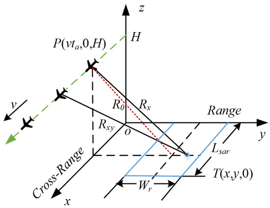
Figure 1. Geometry of the strip-map SAR system.

We consider a radar that transmits a chirp signal

$$s\left(t_r\right)=rect\left(\frac{t_r}{T_p}\right)\exp \left[j2\pi \left(f_c{t}_r+\frac{1}{2}\gamma t_r^2\right)\right],$$

(1)

where $f_c$. and $\gamma$ represent the carrier-frequency and the chirp rate, respectively; $rect(\cdot )$ stands for a rectangular time window; $t_r$ is the fast-time; and $T_p$ is the pulse width. For simplicity, the ROI is modeled as a set of scattering points with a discrete form. Then, the strip-map echo is the superposition of the reflectivity reflections from all scattering points. In this case, the received pulse data, after demodulation, may be expressed as

$$y_{echo}\left(t_a,t_r\right)={\displaystyle \underset{\mathsf{\Omega }}{\iint }g\left(x,y\right){\omega }_r\left(t_r-\frac{2R_{xy}\left(t_a^{}\right)}{c}\right){\omega }_a\left(t_a-x/v\right)}\exp \left(-j\frac{4\pi f_c}{c}{R}_{xy}\left(t_a\right)\right)\exp \left(j\pi \gamma {\left(t_r-\frac{2R_{xy}\left(t_a\right)}{c}\right)}^2\right)dxdy,$$

(2)

where $c$ is the speed of light; $\mathsf{\Omega }$ denotes the illuminated region; $t_a$ is the slow-time; and ${\omega }_a(\cdot )$ and ${\omega }_r(\cdot )$ represent the sampling window in range and cross-range direction, respectively. In (2), $g\left(x,y\right)$ represents the scattering coefficient of an arbitrary point target located at $\left(x,y,0\right)$, and $R_{xy}\left(t_a\right)$ is the instantaneous distance between the radar and the point scatterer $\left(x,y,0\right)$ and can be mathematically expressed as $R_{xy}\left(t_a\right)=\sqrt{R_x^2+{\left(v{t}_a-x\right)}^2}$.

For any ROI placed at the far field of the radar ($R_x\gg \left(v{t}_a-x\right)$), the instantaneous distance $R_{xy}\left(t_a\right)$, based on the Fresnel approximation, may be achieved as

$$R_{xy}\left(t_a\right)\approx R_x+\frac{{\left(v{t}_a-x\right)}^2}{2R_x},$$

(3)

where R_x represents the shortest distance between the point target and the platform.

Generally, the range high resolution can be achieved through implementing pulse compression. Then, the echo after matched filtering can be expressed as

$$y_p\left(t_a,t_r\right)={\displaystyle \underset{\mathsf{\Omega }}{\iint }g\left(x,y\right){\omega }_a\left(t_a-x/v\right)\sin c\left[B(t_r-\frac{2R_{xy}\left(t_a\right)}{c})\right]}\exp \left(-j\frac{4\pi }{\lambda }{R}_{xy}\left(t_a\right)\right)dxdy,$$

(4)

where $B=\gamma T_p$ is the bandwidth of the chirp signal, λ is the wavelength, and $\exp \left(-j\frac{4\pi }{\lambda }{R}_{xy}\left(t_a\right)\right)$ denotes the Doppler shift.

Owing to the influence of the platform movement, the quadratic term in (3) will cause a range migration (range curvature), leaving the range and cross-range dimensions coupled. As such, a range walk correction is required. Specifically, the range migration in (4) can be corrected by scale transformation. Then, (4) becomes

$$y_p\left(t_a,t_r\right)={\displaystyle \underset{\mathsf{\Omega }}{\iint }g\left(x,y\right){\omega }_a\left(t_a-x/v\right)\sin c\left[B(t_r-\frac{2R_x}{c})\right]}\exp \left(-j\frac{4\pi }{\lambda }\left(R_x+\frac{{\left(v{t}_a-x\right)}^2}{2R_x}\right)\right)dxdy,$$

(5)

By inverse transformation, (2) with the range walk removed can be re-expressed as

$$y\left(t_a,t_r\right)={\displaystyle \underset{\mathsf{\Omega }}{\iint }g\left(x,y\right){\omega }_r\left(t_r-\frac{2R_x}{c}\right){\omega }_a\left(t_a-x/v\right)}\exp \left(j\pi \gamma {\left(t_r-\frac{2R_x}{c}\right)}^2\right)\exp \left(-j\frac{4\pi }{\lambda }\left(R_x+\frac{{\left(v{t}_a-x\right)}^2}{2R_x}\right)\right)dxdy,$$

(6)

In the SAR system, the range resolution and the cross-range resolution are defined as ${\rho }_r=c/2B$ and ${\rho }_a\approx D/2$, respectively. As a consequence, the whole range-azimuth plane can be discretized into $\overline{P}\times \overline{Q}$ grids with $x_p=\left(p-1\right){\rho }_a,$ $p=1,2,\cdots \overline{P}$ and $y_q=\left(q-1\right){\rho }_r,$ $q=1,2,\cdots \overline{Q}$.

Assume that M pulses are transmitted during the CPI with the sampling number N for each received pulse. Then, the received signal can be rewritten as

$$\begin{array}{cc}\begin{array}{ll}y\left(t_{a,m},t_{r,n}\right)=& {\displaystyle \sum _{p=1}^{\overline{P}}{\displaystyle \sum _{q=1}^{\overline{Q}}{g}_{pq}{\omega }_a\left(t_{a,m}-\frac{x_p}{v}\right){\omega }_r\left(t_{r,n}-\frac{2R_q}{c}\right)}} \\ & \cdot \exp \left(-j\frac{4\pi }{\lambda }{R}_0\right)\exp \left(j\pi \gamma {\left(t_{r,n}-\frac{2R_q}{c}\right)}^2\right)\cdot \exp \left(-j\frac{2\pi v^2{\left(t_{a,m}-x_p/v\right)}^2}{\lambda R_0}\right)\end{array}& \end{array},$$

(7)

3. Problem Formulation

In this section, we first analyse the TV norm and then induce the TV-based SAR imaging formulation.

TV norm: A key point for the implementation of the SR-based scheme is the selection of a suitable space or dictionary, in which the image can be sparsely represented. In practice, any strip-map SAR imagery possesses a rich smooth structure and texture features. Thus, it is difficult to find a fixed space or dictionary for high precision sparse representation. Fortunately, it is often the case that images are sparse in the finite difference domains or gradient magnitude space. As a result, image reconstruction could be achieved by minimizing the image TV constraint [27]. The g radient space is capable of extracting the edge and texture of the image, which is significantly desired for high resolution SAR imaging. In this section, we investigate the SAR image total variation.

Normally, for any image $G\in {ℝ}^{P\times Q}$, its isotropic TV [28,29] is defined as

$$\mathrm{grad}\left(G\right)={\displaystyle \sum _{i,j}\left({\left|{\nabla }_h^{i,j}G\right|}_1+{\left|{\nabla }_v^{i,j}G\right|}_1\right)},$$

(8)

where ${\Vert \cdot \Vert }_1$ stands for the $l_1$ norm, ${\nabla }_h^{i,j}$ and ${\nabla }_v^{i,j}$ denote the horizontal and vertical first-order difference operators, respectively:

$$\begin{array}{c}\begin{array}{ll}{\nabla }_h^{i,j}G=\{& \begin{array}{l}\begin{array}{cc}{G}_{i+1,j}-G_{i,j},& i<P\end{array}\\ \begin{array}{cc}{G}_{1,j}-G_{P,j},& i=P\end{array}\end{array}\\ {\nabla }_v^{i,j}G=\{& \begin{array}{l}\begin{array}{cc}{G}_{i,j+1}-G_{i,j},& j<Q\end{array}\\ \begin{array}{cc}{G}_{i,1}-G_{i,Q},& j=Q\end{array}\end{array}\end{array}\end{array}.$$

(9)

It may be shown that the sparse decomposition of an image in the gradient space may be performed independently in two orthogonal directions. In the matrix form, (8) can be written as $\mathrm{grad}\left(G\right)={\Vert {\nabla }_{h}G\Vert }_1+{\Vert {\nabla }_{v}G\Vert }_1$.

(1) Random under-sampling scheme: To mitigate the influence of the grid mismatch, we take into account a dense sampling grid in the CS framework. Particularly, a sampling grid of size $P\times Q$ is adopted over the ROI with $P\gg \overline{P}$ and $Q\gg \overline{Q}$. Then, the signal model in (6) can be re-expressed as

$$\begin{array}{cc}\begin{array}{c}y\left(t_{a,m},t_{r,n}\right)={\displaystyle \sum _{p=1}^P{\displaystyle \sum _{q=1}^Q{\phi }_{m,p}\left(t_{a,m}\right)\cdot g_{pq}\cdot {\varphi }_{q,n}}}\left(t_{r,n}\right)\\ where {\phi }_{m,p}\left(t_{a,m}\right)={\omega }_a\left(t_{a,m}-\frac{x_p}{v}\right)\exp \left(-j\frac{2\pi v^2{\left(t_{a,m}-x_p/v\right)}^2}{\lambda R_0}\right)\\ {\varphi }_{q,n}\left(t_{r,n}\right)={\omega }_r\left(t_{r,n}-\frac{2R_q}{c}\right)\exp \left(-j\frac{4\pi }{\lambda }{R}_0\right)\exp \left(j\pi \gamma {\left(t_{r,n}-\frac{2R_q}{c}\right)}^2\right)\end{array}& \end{array},$$

(10)

(10) can be rewritten as the matrix multiplication form:

$$Y=AGB,$$

(11)

where $Y\in {ℂ}^{M\times N}$ is the observation data, and $G\in {ℂ}^{P\times Q}$ is a 2D reflectivity of the ROI. In (10), $A={\left[{\mathbf{\phi }}_1,\dots ,{\mathbf{\phi }}_m,\dots ,{\mathbf{\phi }}_M\right]}^T$ $\in {ℂ}^{M\times P}$ and $B=[{\mathbf{\varphi }}_1,\dots ,{\mathbf{\varphi }}_n\dots ,{\mathbf{\varphi }}_N]\in {ℂ}^{Q\times N}$ denote the cross-range and range sensing matrix, respectively, with ${\mathbf{\phi }}_m={[{\phi }_{m,1}\left(t_{a,m}\right),{\phi }_{m,2}\left(t_{a,m}\right),\dots ,{\phi }_{m,P}\left(t_{a,m}\right)]}^T\in {ℂ}^{P\times 1}$ and ${\mathbf{\varphi }}_n=\left[{\varphi }_{1,n}\left(t_{r,n}\right),{\varphi }_{2,n}\left(t_{r,n}\right),\dots ,{\varphi }_{Q,n}\left(t_{r,n}\right)\right]\in {ℂ}^{Q\times 1}$. Note that ${\mathbf{\phi }}_m$ and ${\mathbf{\varphi }}_n$ are typically independent of each other, which implies that the range and the cross-range dimension are decoupled.

CS theory could recover the signal with a high probability from fewer measurements. As a consequence, an efficient random under-sampling scheme similar to [30] is adopted in this paper. In both the range and cross-range directions, the sampling pattern may be expressed by a random {0,1} sequence denoted by ${\mathit{z}}_r$ and ${\mathit{z}}_a$, respectively. The decimation is implemented first in the cross-range dimension and then in the range dimension. Hence, the random under-sampling matrix $\mathbf{\Phi }$ may be formulated as

$$\Phi ={\Phi }_a\otimes {\Phi }_r^T,$$

(12)

where ${\Phi }_a=diag\left({\mathit{z}}_a\right)\in {ℂ}^{K\times M}$ and ${\Phi }_r=diag\left(z_r\right)\in {ℂ}^{N\times L}$, with K and L being the numbers of the under-sampled measurements in the cross-range and range directions, respectively. Then, based on the properties of the Kronecker product, the under-sampling result of (11) may be formed as

$$\begin{array}{ll}vec\left(Z\right)& =\mathit{z}=\Phi vec\left(Y\right)\\ & =\left({\Phi }_a\otimes {\Phi }_r^T\right)\left(A\otimes B_{}^T\right)vec\left(G\right)\\ & =\left[{\Phi }_{a}A\otimes {\left(B{\Phi }_r\right)}^T\right]vec\left(G\right)\\ & =vec\left({\Phi }_{a}AGB{\Phi }_r\right)\\ & \iff Z=\left( {\Phi }_{a}A\right)G \left(B{\Phi }_r\right)=P_{a}G{P}_r\end{array},$$

(13)

where $\otimes$ denotes the Kronecker product; $vec(\cdot )$ is the operation by stacking the columns of a matrix into a vector, and $P_a={\mathbf{\Phi }}_{a}A$ and $P_r=B{\mathbf{\Phi }}_r$ are known sensing matrices in the cross-range and range directions, respectively. In [6], Candès et al showed that, when the number of linear measurements satisfies $m\ge \mathit{const}\cdot {\mu }^2\left(U\right)\cdot S\cdot \log n$, solving an l₁-norm minimization problem fully recovers a sparse vector. Here, S is the number of nonzero components in x, and μ is the mutual coherence, defined as

$$\mu \left(P\right)=\underset{i,j}{\max }\left|\frac{⟨P_i,P_j⟩}{{\Vert P_i\Vert }^2{\Vert P_j\Vert }^2}\right|,$$

(14)

where $P_i$ denotes the i-th column of the matrix $P$. Equation (11) shows that low mutual coherence results in fewer measurements required for exact signal recovery.

(2) Problem formulation: In the CS framework, the 2D signal is usually converted into a 1D vector for further processing through the Krnoecker product, yielding

$$\mathit{z}=\left( P_a\otimes P_r{}^T\right)\mathit{g}+{\epsilon }_n,$$

(15)

where ${\epsilon }_n$ represents the noise vector and $\mathit{g}=vec\left(G\right)$. In this way, the SAR image formulation problem may be addressed by solving the 1D constrained TV regularization problem

$$\underset{\mathit{g}}{\min } {\Vert \mathit{g}\Vert }_{TV},s.t. {\Vert \mathit{z}-\left( P_a\otimes P_r{}^T\right)\mathit{g}\Vert }_2^2\le \epsilon ,$$

(16)

$$\underset{G}{\min }{\Vert {\nabla }_{h}G\Vert }_1+{\Vert {\nabla }_{v}G\Vert }_1+\frac{\zeta }{2}{\Vert \mathbf{Z}-P_{a}G{P}_r\Vert }_2^2,$$

(17)

where $\zeta$ is the regularized parameter. As noted, the minimization problem in (17) involves multiple $l_1$ regularizer terms, and the $\mathrm{grad}\left(G\right)$ is non-differentiable. Therefore, it is difficult to directly and efficiently solve it. Subsequently, we present an effective numerical algorithm to solve this problem by developing a modified alternating split Bregman method.

4. SAR Imaging Formulation Based on Modified Alternating Split Bregman

The split Bregman technique has shown its superior performance when dealing with a 1D convex optimization problem [28,29]. In this section, we extended the technique to the 2D signal and derived an efficient 2D SAR imaging algorithm based on the modified alternating split Bregman technique.

Specifically, new auxiliary variables $D_h$, $D_v$ and $V$ are introduced by applying the splitting technique, which yields the following constrained problem

$$\begin{array}{l}\underset{G}{\min }\left({\Vert D_h\Vert }_1+{\Vert D_v\Vert }_1+\frac{\zeta }{2}{\Vert \mathbf{Z}-P_{a}G{P}_r\Vert }_2^2\right)\\ s.t.D_h={\nabla }_{h}V,D_v={\nabla }_{v}V,V=G\end{array}$$

(18)

It is noted that problem (18) is equivalent to (17). Owing to the splitting technique, the $l_1$ and $l_2$ terms in (18) are decoupled. Different from [29], an additional auxiliary variable $V$ is introduced here. As a result, the Silvester method can be taken to accelerate the computational speed. In this case, variables $D_h$, $D_v$ and $G$ are separately present in different terms, and are flexible for simple calculation.

To address the problem in (18), we first formulate the constrained optimization problem into an unconstrained one, yielding

$$\underset{G,D_h,D_v,V}{\min }({\Vert D_h\Vert }_1+{\Vert D_v\Vert }_1+\frac{\zeta }{2}{\Vert \mathbf{Z}-P_{a}G{P}_r\Vert }_2^2+\frac{\upsilon }{2}{\Vert V-G\Vert }_2^2+\frac{{\lambda }_1}{2}{\Vert D_h-{\nabla }_{h}V\Vert }_2^2+\frac{{\lambda }_2}{2}{\Vert D_v-{\nabla }_{v}V\Vert }_2^2),$$

(19)

where ${\lambda }_1$, ${\lambda }_2$ and υ represent the regularized parameters. Then, by applying the Bregman iteration procedure, problem (19) is reformulated as

$$\begin{array}{cc}\begin{array}{l}\left(D_h^{k+1},D_v^{k+1},G^{k+1},V^{k+1}\right)=\underset{G,D_h,D_v,V}{\min }({\Vert D_h\Vert }_1+{\Vert D_v\Vert }_1\\ +\frac{\zeta }{2}{\Vert \mathbf{Z}-P_{a}G{P}_r\Vert }_2^2+\frac{\upsilon }{2}{\Vert V-G+W^k\Vert }_2^2\\ +\frac{{\lambda }_1}{2}{\Vert {\nabla }_{h}V-D_h^{}+B_h^k\Vert }_2^2+\frac{{\lambda }_2}{2}{\Vert {\nabla }_{v}V-D_v^{}+B_v^k\Vert }_2^2)\end{array}& \end{array},$$

(20)

$$\begin{array}{cc}\{\begin{array}{l}{W}^{k+1}=W^k+\left(V^{k+1}-G^{k+1}\right)\\ B_v^{k+1}=B_v^k+\left({\nabla }_v{V}^{k+1}-D_v^{k+1}\right)\\ B_h^{k+1}=B_h^k+\left({\nabla }_h{V}^{k+1}-D_h^{k+1}\right)\end{array}& \end{array},$$

(21)

where k and k + 1 represent the k-th and k + 1-th iterations, respectively. Now, the optimization problem (19) is reduced into a sequence of unconstrained optimization problems and Bregman updates. Next, we will show that the procedure for solving (19) is easier and is much more efficient than solving (16).

The problem (20) is a joint optimization problem including several unknown multiple variables, so it is difficult to directly solve. Nevertheless, using the “split” procedure, the problem can be addressed by applying the alternative iteration strategy. Specifically, the problem may be performed by iteratively solving four sub-problems, i.e.,

$$\left(S_1\right):G^{k+1}=\underset{G}{\min }\left\{\frac{\zeta }{2}{\Vert Z-P_{a}G{P}_r\Vert }_2^2+\frac{\upsilon }{2}{\Vert V^k-G+W^k\Vert }_2^2\right\},$$

(22)

$$\begin{array}{cc}\left(S_2\right):V^{k+1}=\underset{V}{\min }\{\frac{{\lambda }_1}{2}{\Vert {\nabla }_{h}V-D_h^k+B_h^k\Vert }_2^2+\frac{{\lambda }_2}{2}\Vert {\nabla }_{v}V-D_v^k{+B_v^k\Vert }_2^2+\frac{\upsilon }{2}{\Vert V-G^{k+1}+W^k\Vert }_2^2\}& \end{array},$$

(23)

$$\left(S_3\right):D_h^{k+1}=\underset{D_h}{\min }\left\{{\Vert D_h^{}\Vert }_1+\frac{{\lambda }_1}{2}{\Vert {\nabla }_h{V}^{k+1}-D_h^{}+B_h^k\Vert }_2^2\right\},$$

(24)

$$\left(S_4\right):D_v^{k+1}=\underset{D_v}{\min }\left\{{\Vert D_v^{}\Vert }_1+\frac{{\lambda }_2}{2}{\Vert {\nabla }_v{V}^{k+1}-D_v^{}+B_v^k\Vert }_2^2\right\}.$$

(25)

Next, efficient strategies are adopted to solve each sub-problem.

4.1. Solving Procedure for $G$

It is noticed that the sub-problem (S₁), which consists of two l₂ regularization terms, is differentiable. Hence, by differentiating with respect to $G$, and setting the result to zero, one may find

$$\zeta \left(P_a^T{P}_a\right)G\left(P_r{P}_r^T\right)+\upsilon G=\zeta P_a^{T}Z{P}_r^T+\upsilon V^k+\upsilon W^k.$$

(26)

Apparently, the right side of (25) is irrelevant to $G$, Thus, (25) is a typical discrete-time Sylvester equation [31]. For simplicity, here, we define ${\Gamma }^k=\zeta P_a^{T}Z{P}_r^T+\upsilon V^k+\upsilon W^k$. Furthermore, by considering that $P_a^T{P}_a$ and $P_r{P}_r^T$ are diagonal matrices, we make an eigen-decomposition over them with $P_a^T{P}_a=U_a^T{\mathbf{\Lambda }}_a{U}_a$ and $P_r{P}_r^T=U_r^T{\mathbf{\Lambda }}_r{U}_r$, where $U_a$ and $U_r$ are orthogonal matrices, and ${\Lambda }_a=diag({\alpha }_1,\dots ,{\alpha }_P)$ and ${\Lambda }_r=diag({\beta }_1,\dots ,{\beta }_Q)$ are diagonal matrices. Then

$$\zeta \left(P_a^T{P}_a\right)G\left(P_r{P}_r^T\right)+\upsilon G={\Gamma }^k.$$

(27)

We next multiply the left side of (26) by $U_a$ and the right side by $U_b^T$, yielding

$$\zeta {\Lambda }_a{U}_{a}G{U}_r^T{\Lambda }_r+\upsilon U_{a}G{U}_r^T=U_a{\Gamma }^k{U}_r^T.$$

(28)

Let $\tilde{G}=U_{a}G{U}_r^T$ and ${\tilde{\Gamma }}^k=U_a{\Gamma }^k{U}_r^T$, then (27) is re-expressed as

$$\zeta {\Lambda }_a\tilde{G}{\Lambda }_r+\upsilon \tilde{G}={\tilde{\Gamma }}^k.$$

(29)

Denoting the (i,j)th entry of $\tilde{G}$ as ${\tilde{g}}_{ij}^{}$ and of $\tilde{\mathbf{\Gamma }}$ as ${\tilde{c}}_{ij}$, then $\zeta {\alpha }_i{\tilde{g}}_{ij}^{}{\beta }_j+\upsilon {\tilde{g}}_{ij}^{}={\tilde{c}}_{ij}^k$. As a result, one may achieve

$${\tilde{g}}_{ij}^{}=\frac{{\tilde{c}}_{ij}^k}{\zeta {\alpha }_i{\beta }_j+\upsilon }.$$

(30)

Finally, once $\tilde{G}$ is achieved, $G^{k+1}$ can be computed by $G^{k+1}=U_a^T\tilde{G}{U}_r$.

4.2. Solving Procedure for $V$

After achieving $G^{k+1}$, we may calculate the auxiliary variables $V^{k+1}$ by solving (S₂). Prior to further processing, we apply some changes that facilitate the subsequent computation. Generally, the differential operators ${\nabla }_h$ and ${\nabla }_v$ may be expressed with the first-order differential matrices in horizontal and vertical directions, ${\Pi }_h$ and ${\Pi }_v$, respectively. Mathematically, ${\nabla }_{h}V={\Pi }_{h}V,$${\nabla }_{v}V=V{\Pi }_v$ with

$${\Pi }_h=\left[\begin{array}{ccccc}-1& 0& \cdots & 0& 1\\ 1& -1& \ddots & \ddots & 0\\ 0& 1& -1& \ddots & ⋮\\ ⋮& \ddots & \ddots & \ddots & 0\\ 0& \cdots & 0& 1& -1\end{array}\right],{\Pi }_v=\left[\begin{array}{ccccc}-1& 1& 0& \cdots & 0\\ 0& -1& 1& \ddots & ⋮\\ ⋮& \ddots & -1& \ddots & 0\\ 0& \ddots & \ddots & \ddots & 1\\ 1& 0& \cdots & 0& -1\end{array}\right].$$

(31)

Moreover, considering that the sub-problem (S₂) is differentiable, the same solving procedure for the matrix $G$ may be applied. Specifically, by setting the derivative of (S₂) with respect to $V$ to zero, we achieve

$$\begin{array}{cc}\begin{array}{c}{\lambda }_1\left({\Pi }_h^T{\Pi }_h\right)V+{\lambda }_{2}V\left({\Pi }_v{\Pi }_v^T\right)+\upsilon V=\\ {\lambda }_1{\Pi }_h^T\left(D_h^k-B_h^k\right)+{\lambda }_2\left(D_v^k-B_v^k\right){\Pi }_v^T+\upsilon \left(G^{k+1}-W^k\right)\end{array}& \end{array},$$

(32)

Apparently, (31) is another discrete-time Sylvester equation for the right side of (26), and is irrelevant to $V$. Thus, the same scheme as that in the analysis of (25) can be adopted here. In particular, we make the eigenvalue decomposition over ${\Pi }_h^T{\Pi }_h$ and ${\Pi }_v{\Pi }_v^T$, respectively, which yields

$$\begin{array}{cc}\{\begin{array}{l}{\Pi }_h^T{\Pi }_h=U_h^T{\Lambda }_h{U}_h\\ {\Pi }_v{\Pi }_v^T=U_v^T{\Lambda }_v{U}_v\end{array}& \end{array},$$

(33)

where $U_h$ and $U_v$ are orthogonal matrices, and ${\Lambda }_h=diag\left({\alpha }_1{}^{\prime },{\alpha }_2{}^{\prime },\cdots {\alpha }_P{}^{\prime }\right)$ and ${\Lambda }_v=diag\left({\beta }_1{}^{\prime },{\beta }_2{}^{\prime },\cdots {\beta }_Q{}^{\prime }\right)$ are diagonal matrices. Then, (31) may be rewritten as

$$\begin{array}{cc}\begin{array}{l}{\lambda }_1\left(U_h^T{\Lambda }_h{U}_h\right)V+{\lambda }_{2}V\left(U_v^T{\Lambda }_v{U}_v\right)+\upsilon V=\\ {\lambda }_1{\Pi }_h^T\left(D_h^k-B_h^k\right)+{\lambda }_2\left(D_v^k-B_v^k\right){\Pi }_v^T+\upsilon \left(G^{k+1}-W^k\right)\end{array}& \end{array}.$$

(34)

Similarly, we define $H_{}^k={\lambda }_1 {\Pi }_h^T\left(D_h^k-B_h^k\right)+{\lambda }_2\left(D_v^k-B_v^k\right){\Pi }_v^T$,$+\upsilon \left(G^{k+1}-W^k\right)$, which is irrelevant to the $V$ and may be treated as a constant. Multiplying the left hand of (33) by $U_h$ and its right hand by $U_v^T$, we achieve

$${\lambda }_1{\Lambda }_h{U}_{h}V{U}_v^T+{\lambda }_2{U}_{h}V{U}_v^T{\Lambda }_v+\upsilon U_{h}V{U}_v^T=U_h H_{}^k{U}_v^T.$$

(35)

Let ${\tilde{H}}_{}^k=U_h{H}_{}^k{U}_v^T$, $\tilde{V}=U_{h}V{U}_v^T$ and denote the (i,j)th entry of $\tilde{V}$ and ${\tilde{H}}^k$ as ${\tilde{v}}_{ij}$ and ${\tilde{h}}_{ij}^k$, respectively. Next, one may achieve

$${\tilde{v}}_{ij}=\frac{{\tilde{h}}_{ij}^k}{\upsilon +\lambda {\alpha }_{ii}{}^{\prime }+\lambda {\beta }_{jj}{}^{\prime }}.$$

(36)

Finally, once we compute $\tilde{V}$, $V^{k+1}$ may be calculated using $V^{k+1}=U_h^T\tilde{V}{U}_v$.

4.3. Solving Procedure for $D_h$ and $D_v$

As noted, the solution of $D_h^{k+1}$ and $D_v^{k+1}$ may be directly computed via the iterative shrinkage method [24], and the estimation results during the iteration may be expressed as

$${\left(D_h^{k+1}\right)}_{i,j}=shrink\left({\left({\nabla }_h{V}^{k+1}+B_h^k\right)}_{i,j},\frac{1}{{\lambda }_1}\right),$$

(37)

$${\left(D_v^{k+1}\right)}_{i,j}=shrink\left({\left({\nabla }_v{V}^{k+1}+B_v^k\right)}_{i,j},\frac{1}{{\lambda }_2}\right),$$

(38)

where $shrink\left(x,\overline{\gamma }\right)=sign\left(x\right)\ast \max \left(\left|x\right|-\overline{\gamma },0\right)$ is a classic soft-thresholding operator possessing an extremely fast computation procedure. For the detailed derivation of (36) and (37), one may refer to [24].

Finally, we derive the SAR imaging algorithm based on the modified alternating split Bregman (MASB) algorithm. Algorithm 1 illustrates the details of the flow.

Algorithm 1. Procedure of the proposed MASB imaging algorithm.

Input: 2-D signal y; Step 1: Range Migration Correction Implement pulse compression over the input signal, then operate range walk correction through scale transformation, Finally implement inversion match filtering to achieve the signal y; Step 2: 2-D radar imaging Initialization: set $W^0$,$G^0$, $B_{\mathrm{h}}^0$ and $B_v^0$ be zero, $V^0$, $D_{\mathrm{h}}^0$ and $D_v^0$ as an identity matrix, k = 0; initial value of parameters {${\zeta }^0$, ${\lambda }_1^0$${\lambda }_2^0$, ${\upsilon }^0$ } repeat 1. Estimate $G^{k+1}$ via (29); 2. Estimate $V^{k+1}$ via (35); 3. Estimate $D_h^{k+1}$ and $D_v^{k+1}$ via (36) and (37); 4. Update the $B_h^k$,$B_v^k$ and $W^k$  via (20); End Until convergence Output $G=G^{k+1}$

Particularly, this iterative will be repeated until the residual ${{\Vert G^{k+1}-G^k\Vert }_2^2/\Vert G^{k+1}\Vert }_2^2$ is lower than a predefined threshold tol. In comparison with the traditional CS-based SAR imaging algorithm, the proposed one exhibits a set of potential merits. First, the proposed algorithm is implemented over the separable sensing structures, which greatly reduces the computational cost and storage memory. As a consequence, it provides a feasible way to deal with a large-scale SAR image reconstruction problem. Second, instead of solving a nonlinear system of equations, the modified alternating split Bregman scheme requires a simpler mathematical computation, and thus exhibits superior efficiency. In addition, both sensing matrixes, $P_a$ and $P_r$, and differential matrices ${\Pi }_h^{}$ and ${\Pi }_v$, are irrelevant to the strip-map SAR scene. In other words, the matrices $U_a$, $U_r$, ${\Lambda }_a$,${\Lambda }_r$, $U_h$, $U_v$, ${\Lambda }_h$, ${\Lambda }_v$ are independent of the reconstruction signal, and may be calculated in advanced. For these reasons, the proposed algorithm is more competitive for the strip-map SAR in practice. Subsequently, we will demonstrate it via simulations.

4.4. Parameter Selection

As shown in Algorithm1, regularization parameters ${\lambda }_1$, ${\lambda }_2$, $\zeta$ and $\upsilon$ need to be identified in the implementation of the proposed algorithm. Actually, these parameters can be chosen by adopting the L-curve method [32,33]. To be specific, the theory of the L-curve indicates that the plotted curves of the regularizer term versus the fidelity term for different regularization parameters share an “L”-shape, and the optimal regularization parameter is the one corresponding to the corner in the L-curve. Motivated by it, the regularization parameter can be selected by the L-curve method. As the imaging problem (19) is split into four sub-problems, parameters can be determined one by one. The parameter $\upsilon$ can be estimated from (21). Then, the optimal $\upsilon$ is found as the corner of the L-curve, which consists of plotting $\log {\Vert D_h^{}\Vert }_1$ as a function of $\log \frac{1}{2}\Vert {\nabla }_h{V}^{k+1}-D_h^{}+B_h^k\Vert$. Similarly, other parameters, ${\lambda }_1$, ${\lambda }_2$ and $\zeta$ can be estimated from (22)–(24), respectively. In fact, the proposed algorithm is not sensitive to the parameter selection, and it could exhibit relatively consistent results for different parameter selection. The reason is mainly that the bias induced by regularized parameters is “removed” when the Bregman parameter is updated. The idea is similar to the “adding back the noise” in the optimization formulation for TV denoising [29]. The error is added back to the iteration through updating the Bregman parameter. This allows some freedom in fitting the data even for an improper set of parameters. Simulation results are given in the simulation to demonstrate this.

4.5. Computational Complexity

The computational complexity of the proposed algorithm mainly stems from three parts, i.e., estimation of the reflectivity field $G$, estimation of $V$ and calculation of the gradient images $D_h$ and $D_v$. Considering $K$ and $L$ as the numbers of the samplers in the range and cross-range directions, the computational complexity for the estimation of the reflectivity field $G$ needs $O\left(P^{2}Q+P{Q}^2+PKL+PQL\right)$. While the estimation of $V$ requires $O\left(P^{2}Q+P{Q}^2+PQ\right)$ operations. By comparison, the calculation of the gradient image $D_h$ and $D_v$ only requires $O\left(PQ\right)$ operations. The whole computational complexity of the proposed algorithm is approximated as $O\left(I_{ter}\ast \left(P^{2}Q+P{Q}^2+PKL+PQL\right)\right)$, where $I_{ter}$ corresponds to the iteration number.

Next, we compare the memory cost with respect to the proposed image formulation algorithm and the conventional CS-based scheme. More specifically, for an image of size $P\times Q$, according to the conventional CS-based scheme, the scale of the basis for the sparse representation reads $PQ\times PQ$. Considering a complex number occupying 16 bits of memory, the memory cost for storing such a large-scale basis is $16P^2{Q}^2$ bits. Since in the proposed algorithm, the scales of the bases are reduced to $P\times P$ and $Q\times Q$, the total memory cost for storing bases is $16\left(P^2+Q^2\right)$ bits. For instance, if $P=Q=K=L=512$, the conventional CS-based scheme requires 1TB memory to store the basis matrix. However, the memory cost of the proposed algorithm requires 8 MB.

5. Simulations and Result Analysis

We conduct several simulations to assess the performance of the proposed image formulation algorithm. Here, the RD algorithm and the traditional CS-based SAR image formulation algorithm (called TCS-SAR here) are taken for comparison. To be fair, we adopt an effective and similar scheme [18] by taking the variable-splitting and penalty technique to solve the following induced problem:

$$\underset{\mathit{g}}{\min }{\displaystyle \sum _i{\left|{\mathit{w}}_i\right|}_1}+\frac{\zeta }{2}{\Vert \mathit{z}-\left( P_a\otimes P_r{}^T\right)\mathit{g}\Vert }_2^2+\frac{\lambda }{2}{\Vert {\mathit{D}}_i\mathit{g}-{\mathit{w}}_i\Vert }_2^2,$$

(39)

where ${\mathit{w}}_i$ is an induced auxiliary variable and ${\mathit{D}}_i\mathit{g}$ represents the discrete gradient of g at the pixel i. It is clear that (38) shares similar penalty parameters and may be solved through minimizing the objective function with respect to one of the two variables $\mathit{g}$ and $\mathit{w}$, where the other one is fixed. The initial parameters $\zeta$ and $\lambda$ for the TCS-SAR are set using the L-curve method. Table 1 lists the primary radar parameters used for the simulations. Furthermore, we evaluate the reconstructed performance by two image quality metrics, peak signal to noise ratio (PSNR) and structural similarity (SSIM) [34], as follows:

Table 1. Simulation Parameters.

Center frequency	10 GHz
Bandwidth	150 MHz
Pulse time interval	5 μs
Radar velocity	150 m/s
Squint angle	0°
Aperture	3 m
Pulse repetition frequency	100 Hz
Slant range of scene center	20 km
Swath	3000 m
Range resolution	1 m
Cross-range resolution	1.5 m

(1)

Peak signal to noise ratio is represented by

$$\begin{array}{cc}\begin{array}{l}\mathrm{PSNR}=-10lg\left(\mathrm{MSE}/{\rho }_{\max }\right)\\ \mathrm{MSE}=\frac{1}{PQ}{\displaystyle \sum _{j=1}^Q{\displaystyle \sum _{i=1}^P{\left({\mathit{g}}_{i,j}-{\widehat{\mathit{g}}}_{i,j}\right)}^2}}\end{array}& \end{array},$$

(40)

where $\mathit{g}$ and $\widehat{\mathit{g}}$ represent the original image and the reconstructed one, respectively, and ${\rho }_{\max }$ denotes the maximum value of the noisy image.

(2)

Structural similarity is defined as

$$\mathrm{S} \mathrm{SIM}=\frac{\left(2u_{\mathit{g}}{u}_{\widehat{\mathit{g}}}+H_1\right)\left(2{\sigma }_{\mathit{g}\widehat{\mathit{g}}}+H_2\right)}{\left(u_{\mathit{g}}^2{\widehat{u}}_{\widehat{\mathit{g}}}^2+H_1\right)\left(2{\sigma }_{\mathit{g}}^2{\sigma }_{\widehat{\mathit{g}}}^2+H_2\right)},$$

(41)

where $u_{\mathit{g}}$ and ${\sigma }_{\mathit{g}}^2$ are the mean and variance of the image g, respectively, and ${\sigma }_{\mathit{g}\widehat{\mathit{g}}}$ is the covariance between $\mathit{g}$ and $\widehat{\mathit{g}}$. Two variables $H_1$ and $H_2$ are used to stabilize the division with a weak denominator. In general, a larger PSNR results in a better reconstruction and a higher SSIM corresponds to a closer image to the original one. For convenience, empirical values ${\zeta }_{}^{\left(0\right)}=100$, ${\lambda }_1^{\left(0\right)}=50$, ${\lambda }_2^{\left(0\right)}=50$ and ${\upsilon }^{\left(0\right)}=5$ are adopted in the simulation. In particular, all simulations are implemented on a computer with an Intel 3.4-GHz dual core processor and 4GB of RAM.

5.1. Simulation 1

The first experiment is performed to test the capability of the proposed algorithm in achieving high resolution. Table 1 enumerates the primary radar parameters, and a field scene of size 80 × 80 is chosen for the test. By applying the random under-sampling strategy mentioned in Section 3, 25% of the Nyquist rates samples in the range and 33% of the Nyquist rates samples in the cross-range are adopted. This means that only 8.3% of full aperture data have been used for the reconstruction. The signal-to-noise ratio (SNR) is 10 dB and the minimum intervals in the range and the cross-range directions are equal to the range resolution and the cross-range resolution, respectively. Figure 2 displays the RD image with full echo data.

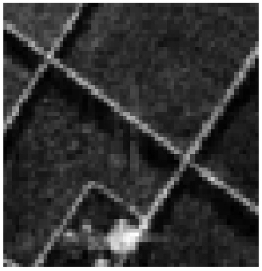
Figure 2. The RD image with full echo data.

Figure 3a,b depict the mutual coherence curves in the range and the cross-range directions, respectively. As shown in Figure 3, the maximum values of the correlation coefficients in the range and the cross-range directions are around the magnitude of −20 dB and −10 dB, respectively, which are both sufficiently small to guarantee a high probability for the reconstruction of the SAR image. Figure 4 displays the reconstructed results achieved using the RD algorithm, TCS-SAR, and the proposed algorithm, respectively. As shown in Figure 4, the image reconstructed by the RD algorithm is seriously merged and difficult to distinguish. The main reason is that the sampling strategy does not satisfy the Nyquist theorem. In contrast, both the TCS-SAR and the proposed algorithm provide excellent performance from under-sampling measurements, which is consistent with the analysis of Figure 4. Additionally, the proposed algorithm provides stronger interference suppression and a superior reconstructed result.

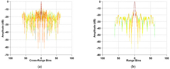
Figure 3. (a) The mutual coherence in the cross-range direction. (b) The mutual coherence in the range direction.

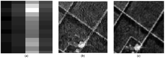
Figure 4. Comparison of the reconstructed results. (a) RD image. (b) TCS-SAR image. (c) Proposed algorithm.

Figure 5 displays the computational time of TCS-SAR and the proposed algorithm, respectively. It is clear that, to reach the same preset threshold tol = 5 × 10⁻⁴, a computational time of up to 800 s is required for TCS-SAR. However, the computational time required by the proposed algorithm is only 0.7 s. As a consequence, the proposed algorithm is obviously more efficient than its competitor. The main reason is that, compared with the vectorization process, by applying the separable sensing structure, the computational cost will be significantly reduced.

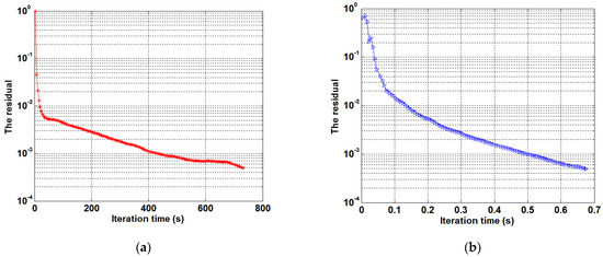
Figure 5. Comparison of the computation time for different algorithms. (a) TCS-SAR. (b) Proposed algorithm.

5.2. Simulation 2

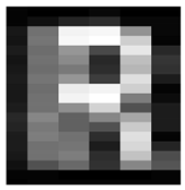
We next investigate the reconstruction precision for different SNRs to further verify the capability of the proposed algorithm. Suppose that the simulated scenes of the letter “R” are corrupted by the white Gaussian noise with SNR varying from −10 dB to 0 dB. During the simulation, we set the pixel intervals in the cross-range and the range directions as 0.66 m and 0.9 m, respectively, which are smaller than the cross-range resolution and range resolution. Similar radar parameters are taken as used previously. Table 2 shows the reconstructed images under different SNRs.

Table 2. Comparison of the imaging results for different SNRs of −0 dB, −4 dB, −8 dB and −10 dB.

Methods	0 dB	−4 dB	−8 dB	−10 dB
RD
TCS-SAR
Proposed

From Table 2, it may be seen that the RD algorithm provides the poorest performance under different SNRs, where the reconstructed images suffer from high side-lobes and are deemed to be blurred. TCS-SAR and the proposed algorithm significantly mitigate the grating lobes, and thus present better performances. However, as the noise increased, the proposed algorithm exhibits superior performance over TCS-SAR.

5.3. Simulation 3

To best show the universality of the proposed algorithm, we conduct different simulations for various sampling rates over a set of SAR images. Table 3 lists three sampling modes, and Figure 6 enumerates the test images. For a more comprehensive comparison and to best evaluate the reconstruction results, we employ multiple metrics, including the PSNR, SSIM, and reconstruction time. Table 4 lists the detailed performance comparisons. Furthermore, all the other parameters remain unchanged from the first experiment.

Table 3. Setting of the under-sampling modes.

Under-Sampling Modes	Direction	The Ratio of the Sampling Rates and Nyquist Rate (%)
Mode I	range	40%
Mode II	Cross-range	25%
Mode III	range and cross-range	33% in range, 25% in cross-range

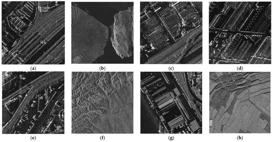
Figure 6. Test images. (a) Image 1; (b) Image 2; (c) Image 3; (d) Image 4; (e) Image 5; (f) Image 6; (g) Image 7; (h) Image 8.

Table 4. Quality metrics for reconstructed images.

Figures	Sampling Mode	TCS-SAR			Proposed
		PSNR (dB)	SSIM	Time (s)	PSNR (dB)	SSIM	Time (s)
Image 1	Mode I	30.36	0.73	210.43	32.98	0.91	0.45
	Mode II	30.00d	0.65	462.94	31.62	0.82	0.49
	Mode III	29.60	0.56	206.95	30.91	0.72	0.43
Image 2	Mode I	34.81	0.85	178.07	39.02	0.97	0.31
	Mode II	30.89	0.54	455.39	36.06	0.94	0.42
	Mode III	30.13	0.47	210.11	35.29	0.92	0.40
Image 3	Mode I	32.59	0.88	185.10	35.51	0.95	0.44
	Mode II	30.22	0.68	389.48	32.58	0.86	0.52
	Mode III	29.73	0.61	202.38	32.09	0.83	0.45
Image 4	Mode I	32.15	0.90	144.67	34.54	0.95	0.49
	Mode II	30.92	0.78	343.44	32.06	0.88	0.54
	Mode III	29.47	0.57	234.37	30.35	0.74	0.54
Image 5	Mode I	35.38	0.88	153.01	35.61	0.94	0.47
	Mode II	30.70	0.68	444.99	33.00	0.87	0.56
	Mode III	29.44	0.61	180.21	31.13	0.81	0.52
Image 6	Mode I	31.60	0.87	185.23	33.71	0.94	0.47
	Mode II	29.69	0.59	452.26	31.42	0.79	0.55
	Mode III	29.56	0.63	212.79	31.41	0.81	0.48
Image 7	Mode I	30.81	0.85	119.36	32.44	0.93	0.36
	Mode II	29.44	0.63	327.07	30.58	0.79	0.40
	Mode III	28.91	0.47	196.51	29.82	0.69	0.37
Image 8	Mode I	32.09	0.92	170.57	33.76	0.96	0.43
	Mode II	29.54	0.76	307.96	31.12	0.88	0.50
	Mode III	29.53	0.72	174.77	30.76	0.86	0.49
Average	Mode I	32.62	0.86	168.91	34.98	0.94	0.42
	Mode II	30.31	0.66	388.26	32.77	0.86	0.49

As shown in Table 4, the proposed algorithm greatly outperforms the TCS-SAR algorithm over all test images and sampling modes. More specifically, in terms of the PSNR, the maximum gap between the proposed algorithm and the TCS-SAR algorithm is 5.17 dB. The average PSNR gains over the comparison algorithms can be up to 2.36 dB, 2.46 dB, and 2.18 dB for Mode I, Mode II, and Mode III, respectively. In addition, as the metric SSIM is more conformed to the human eye visual characteristic, i.e., a higher SSIM value corresponds to a better restoration, the SSIM result also manifests the great benefit of the proposed algorithm.

Moreover, the comparison result of the running time is also appealing. For different sampling modes, the proposed algorithm requires less running time, while for the TCS-SAR algorithm, the largest time cost is already 900 times than that of the proposed algorithm. This is a strong indication of the feasibility of the proposed algorithm in practical SAR applications. The superiority is mainly due to the adopted separable sensing structure and the modified alternating split Bregman scheme.

5.4. Simulation 4

Finally, we apply the proposed algorithm to real SAR data. The primary radar parameters are listed in Table 5. According to the radar parameters, the resolutions in the range and the cross-range directions are 1.5 m. The size of the scene is 650 × 400. To demonstrate the capability of the proposed algorithm, we set the pixel resolutions to 0.3 m and 0.6 m in the range and the cross-range directions, respectively. Then, the demodulated echo is generated according to the real SAR parameters, as listed in Table 5. Note that the sampling rate strictly follows the Nyquist theorem. Figure 7 presents the final reconstructed SAR images by the RD algorithm and the proposed algorithm, where the close-up views of the selected local area in the red window are shown for comparison. Considering the fact that the scale of the basis and the time consumption for the TCS-SAR algorithm are too large, we do not take it into account for comparison.

Table 5. Real SAR parameters.

Center Frequency	15 GHz
Bandwidth	100 MHz
Pulse time interval	2 μs
Radar velocity	120 m/s
Aperture	3 m
Pulse repetition frequency	160 Hz
Slant range of scene center	5 km
Range resolution	1.5 m
Cross-range resolution	1.5 m

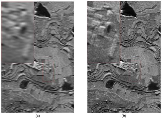
Figure 7. Reconstruction comparison of the real scene. (a) RD algorithm. (b) Proposed algorithm.

It may be seen from Figure 7 that most of the content of the scene is preserved in both test algorithms. However, limited by the signal bandwidth and aperture size, the reconstructed result achieved by the RD algorithm suffers from significant ambiguity. Specifically, only a coarse outline of the scene is available in the result reconstructed by the RD algorithm, and the textures of the terraced and roads in the red rectangle window are seriously merged, which is hard to distinguish. In contrast, all these artifacts are effectively suppressed in the image reconstruction by the proposed algorithm, and a sharp and clear visual result is achieved.

6. Discussion

High resolution performance of the conventional SAR imaging method requires a large signal bandwidth and a long CPI, introducing a great challenge to data acquisition and storage. Thus, high resolution SAR imaging with limited bandwidth and aperture is a hot issue in SAR imaging systems.

By virtue of its powerful capability in terms of high resolution and low data acquisition demand, SR or CS theory is widely used in SAR imaging systems. Usually, the SAR imaging problem is formulated into the sparse signal recovery problem (usually l₁ regularization problem), and then the SAR image is achieved by solving the l₁ regularization problem. However, the available CS-based SAR imaging method suffers from a heavy computational burden, which greatly limits its wide use in practice. One of the important reasons is that the 2D signal reconstruction problem is usually recast as a 1D sparse signal recovery problem by reshaping the 2D matrix into a long vector. The vectorized procedure is always accompanied by a very large matrix, thus the recovery procedure, even for a moderate size scene, is quite time consuming. Therefore, it is a challenge to reduce the computational complexity in the available CS-based SAR imaging system.

Many scholars have made great effort and developed different strategies to accelerate the imaging speed. One way is to improve the construction algorithm by utilizing the special structures of the matrix to avoid the inversion operation. Another way is to expand the l₀ norm approach into a 2D version and propose a 2D smoothed l₀ norm (2D-SL0), which can deal with 2D signal directly, and thus can achieve 2D signal reconstruction efficiently. The second strategy provides a superior performance when the scene is spatially sparse or consists of some dominant scatters. However, the performance degrades for the real SAR scene, drastically changing across the ROI.

We formulate SAR imaging as solving a 2D sparse signal reconstruction problem, where the TV constraint is incorporated to maintain contour information. The induced algorithm can deal with 2D signal directly, leading to a reduced computational load. Further, by developing the MSBL method, the complex optimization problem is developed into a series of sub-problems, yielding accurate and simple solutions without any matrix inversion operations. As shown in Figure 3, the proposed algorithm performed better than the traditional RD algorithm, slightly superior to TCS. Additionally, the computational time was evaluated. As shown in Figure 5, compared with competitors, the proposed algorithm required less computational time and exhibited great potential in practice. Besides, Simulation 4 was designed to show the universality of the proposed algorithm, where eight remote sensing images and two sampling modes were adopted. Apparently, the results displayed in Table 4 came to a similar conclusion. We also applied the algorithm to deal with the real data related to a moderate size scene. The TCS-SAR algorithm cannot be executed because of the enormous calculation, while the proposed algorithm performs well.

7. Conclusions

This paper proposed a CS-based image formulation algorithm for the strip-map SAR with zero squint angle based on the modified alternating split Bregman method. Compared with the conventional l₁ regularization method, the proposed algorithm can deal with 2D signal directly instead of converting it into a 1D vector, which can reduce the computational load significantly. Besides, the TV constraint was engaged to improve image resolution and a modified alternating split Bregman method was developed to accelerate the computational speed. The final simulation results verified the superior performance of the proposed algorithm.

However, in practice, most SAR systems work under the case with a nonzero squint angle. Hence, we will extend the available work to a more realistic scenario where a nonzero squint angle is considered in the future. In addition, we have proven and verified the feasible and superior performance of the proposed algorithm theoretically in this manuscript, while the imaging capability of the proposed algorithm in the real SAR environment remains to be verified. Thus, the real hardware environment will be implemented and a more comprehensive analysis will be investigated in the future.

References

- Chen, Y.C.; Li, G.; Zhang, Q.; Zhang, Q.J.; Xia, X.G. Motion Compensation for Airborne SAR via Parametric Sparse Representation. IEEE Trans. Geosci. Remote Sens. 2017, 55, 551–562. [Google Scholar] [CrossRef]
- Moreira, A.; Prats-Iraola, P.; Younis, M.; Krieger, G.; Hajnsek, I.; Papathanassiou, K.P. A tutorial on synthetic aperture radar. IEEE Geosci. Remote Sens. Mag. 2013, 1, 6–43. [Google Scholar] [CrossRef] [Green Version]
- Donoho, D.L.; Elad, M.; Temlyakov, V.N. Stable recovery of sparse overcomplete representations in the presence of noise. IEEE Trans. Inf. Theory 2006, 52, 6–18. [Google Scholar] [CrossRef]
- Elad, M.; Figueiredo, M.A.T.; Ma, Y. On the role of sparse and redundant representations in image processing. Proc. IEEE 2010, 98, 972–982. [Google Scholar] [CrossRef]
- Donoho, D. Compressed sensing. IEEE Trans. Inf. Theory 2006, 52, 1289–1306. [Google Scholar] [CrossRef]
- Cands, E.J.; Romberg, J.; Tao, T. Robust uncertainty principles: Exact signal reconstruction from highly incomplete frequency information. IEEE Trans. Inf. Theory 2006, 52, 489–509. [Google Scholar] [CrossRef] [Green Version]
- Okeke, G.A.; Abbas, M.; Sen, M. Inertial Subgradient Extragradient Methods for Solving Variational Inequality Problems and Fixed Point Problems. Axioms 2020, 9, 51. [Google Scholar] [CrossRef]
- Candès, E.J.; Wakin, M.B.; Boyd, S.P. Enhancing sparsity by reweighted 1 minimization. J. Fourier Anal. Appl. 2007, 14, 877–905. [Google Scholar] [CrossRef]
- Tibshirani, R. Regression shrinkage and selection via the lasso: A retrospective. J. R. Stat. Soc. Ser. B 2011, 73, 267–288. [Google Scholar] [CrossRef]
- Zhang, Q.; Zhang, Y.; Huang, Y.; Zhang, Y. Azimuth superresolution of forward-looking radar imaging which relies on linearized Bregman. IEEE J. Sel. Top. Appl. Earth Obs. Remote Sens. 2019, 12, 2032–2043. [Google Scholar] [CrossRef]
- Dudczyk, J.; Kawalec, A. Optimizing the minimum cost flow algorithm for the phase unwrapping process in SAR radar. Bull. Pol. Acad. Sci. Tech. Sci. 2014, 62, 511–516. [Google Scholar] [CrossRef] [Green Version]
- Huo, W.; Zhang, Q.; Zhang, Y.; Zhang, Y.; Huang, Y.; Yang, J. A Superfast Super-Resolution Method for Radar Forward-Looking Imaging. Sensors 2021, 21, 817. [Google Scholar] [CrossRef] [PubMed]
- Xiao, D.; Zhang, Y. A Novel Compressive Sensing Algorithm for SAR Imaging. IEEE J. Sel. Top. Appl. Earth Observ. Remote Sens 2014, 7, 708–720. [Google Scholar]
- Önhon, N.Ö.; Çetin, M. A sparsity-driven approach for joint SAR imaging and phase error correction. IEEE Trans. Image Process. 2012, 21, 2075–2088. [Google Scholar] [CrossRef]
- Yang, J.; Thompson, J.; Huang, X.; Jin, T.; Zhou, Z. Segmented reconstruction for compressed sensing SAR imaging. IEEE Trans. Geosci. Remote Sens. 2013, 51, 4214–4225. [Google Scholar] [CrossRef]
- Hyder, M.M.; Mahata, K. Range-Doppler imaging via sparse representation. In Proceedings of the 2011 IEEE RadarCon (RADAR), Kansas City, MO, USA, 23–27 May 2011; pp. 486–491. [Google Scholar]
- Qiu, W.; Zhao, H.; Zhou, J.; Fu, Q. High-resolution fully polarimetric ISAR imaging based on compressive sensing. IEEE Trans. Geosci. Remote Sens. 2014, 52, 6119–6131. [Google Scholar] [CrossRef]
- Zhang, S.; Dong, G.; Kuang, G. Superresolution downward-looking linear array three-dimensional SAR imaging based on two-dimensional compressive sensing. IEEE J. Sel. Top. Appl. Earth Obs. Remote Sens. 2016, 9, 2184–2196. [Google Scholar] [CrossRef]
- Rudin, L.; Osher, S.; Fatemi, E. Nonlinear total variation based noise removal algorithms. Physica. D 1992, 60, 259–268. [Google Scholar] [CrossRef]
- Wang, Y.; Yang, J.; Yin, W.; Zhang, Y. A New Alternating Minimization Algorithm for Total Variation Image Reconstruction. Siam J. Imaging Sci. 2008, 1, 248–272. [Google Scholar] [CrossRef]
- He, W.; Zhang, H.; Zhang, L.; Shen, H. Total-Variation -Regularized Low-Rank Matrix Factorization for Hyperspectral Image Restoration. IEEE Trans. Geosci. Remote Sens. 2016, 54, 178–188. [Google Scholar] [CrossRef]
- Chen, Y.; He, W.; Yokoya, N.; Huang, T.-Z. Hyperspectral Image Restoration Using Weighted Group Sparsity-Regularized Low-Rank Tensor Decomposition. IEEE Trans. Cybern. 2020, 50, 3556–3570. [Google Scholar] [CrossRef] [PubMed]
- Zhang, Y.; Tuo, X.; Huang, Y.; Yang, J. A TV Forward-Looking Super-Resolution Imaging Method Based on TSVD Strategy for Scanning Radar. IEEE Trans. Geosci. Remote Sens. 2020, 58, 4517–4528. [Google Scholar] [CrossRef]
- Esser, E.; Guasch, L.; van Leeuwen, T.; Aravkin, A.Y.; Herrmann, F.J. Total variation regularization strategies in full-waveform inversion. SIAM J. Imaging Sci. 2018, 11, 376–406. [Google Scholar] [CrossRef]
- Zhang, Q.; Zhang, Y.; Huang, Y.; Zhang, Y.; Pei, J.; Yi, Q.; Li, W.; Yang, J. TV-Sparse Super-Resolution Method for Radar Forward-Looking Imaging. IEEE Trans. Geosci. Remote Sens. 2020, 58, 6534–6549. [Google Scholar] [CrossRef]
- Plonka, G.; Jianwei, M.A. Curvelet-Wavelet Regularized Split Bregman Iteration for Compressed Sensing. Int. J. Wavelets Multiresolution Inf. Process. 2011, 9, 79–110. [Google Scholar] [CrossRef] [Green Version]
- Sidky, E.Y.; Pan, X. Image reconstruction in circular cone-beam computed tomography by constrained, total-variation minimization. Phys. Med. Biol. 2008, 53, 4777. [Google Scholar] [CrossRef] [Green Version]
- Osher, S.; Burger, M.; Goldfarb, D.; Xu, J.; Yin, W. An iterative regularization method for total variation-based image restoration. Multiscale Modeling Simul. 2005, 4, 460–489. [Google Scholar] [CrossRef]
- Goldstein, T.; Osher, S. The split Bregman method for L1 regularized problems. SIAM J. Imaging Sci. 2009, 2, 323–343. [Google Scholar] [CrossRef]
- Shen, F.; Zhao, G.; Liu, Z.; Shi, G.; Lin, J. SAR Imaging With Structural Sparse Representation. IEEE J. Sel. Top. Appl. Earth Obs. Remote Sens. 2017, 8, 3902–3910. [Google Scholar] [CrossRef]
- Jameson, A. Solution of the Equation AX + XB = C by Inversion of an M × M or N × N Matrix. Siam J. Appl. Math. 1968, 16, 1020–1023. [Google Scholar] [CrossRef]
- Hansen, P.C. The L-curve and its use in the numerical treatment of inverse problems. Comput. Inverse Problems Electrocardiol. 1999, 51, 119–142. [Google Scholar]
- Calvetti, D.; Reichel, L.; Shuibi, A. L-curve and curvature bounds for Tikhonov regularization. Numer. Algorithms 2004, 35, 301–314. [Google Scholar] [CrossRef]
- Wang, Z.; Bovik, A.C.; Sheikh, H.R.; Simoncelli, E.P. Image quality assessment: From error visibility to structural similarity. IEEE Trans. Image Process 2004, 13, 600–612. [Google Scholar] [CrossRef] [PubMed] [Green Version]
Publisher’s Note: MDPI stays neutral with regard to jurisdictional claims in published maps and institutional affiliations. |
© 2021 by the authors. Licensee MDPI, Basel, Switzerland. This article is an open access article distributed under the terms and conditions of the Creative Commons Attribution (CC BY) license (https://creativecommons.org/licenses/by/4.0/).