Article

Detailed Characterization and Monitoring of a Retrogressive Thaw Slump from Remotely Piloted Aircraft Systems and Identifying Associated Influence on Carbon and Nitrogen Export

by
Kevin W. Turner
1,*,
Michelle D. Pearce
1 and
Daniel D. Hughes
2
1
Department of Geography and Tourism Studies, Brock University, 1812 Sir Isaac Brock Way, St. Catharines, ON L2S 3A1, Canada
2
Canadian Wildlife Health Cooperative, University of Guelph, 50 Stone Road E, Guelph, ON N1G 2W1, Canada
*
Author to whom correspondence should be addressed.
Remote Sens. 2021, 13(2), 171; https://doi.org/10.3390/rs13020171
Submission received: 28 September 2020 / Revised: 27 December 2020 / Accepted: 28 December 2020 / Published: 6 January 2021

Abstract

:
Ice-rich permafrost landscapes are sensitive to ongoing changes in climate. Permafrost retrogressive thaw slumps (RTSs) represent one of the more abrupt and prolonged disturbances, which occur along Arctic river and lake shorelines. These features impact local travel and infrastructure, and there are many questions regarding associated impacts on biogeochemical cycling. Predicting the duration and magnitude of impacts requires that we enhance our knowledge of RTS geomorphological drivers and rates of change. Here we demonstrate the utility of remotely piloted aircraft systems (RPAS) for documenting the volumetric change, associated drivers and potential impacts of the largest active RTS along the Old Crow River in Old Crow Flats, Yukon, Canada. RPAS surveys revealed that 29,174 m3 of sediment was exported during the initial evacuation in June 2016 and an additional 18,845 m3 continued to be exported until June 2019. More sediment export occurred during the warmer 2017 summer that experienced less cumulative rainfall than summer 2018. However, several rain events during 2017 were of higher intensity than during 2018. Overall mean soil organic carbon (SOC) and total nitrogen (TN) within sampled thaw slump sediment was 1.36% and 0.11%, respectively. A combination of multispectral, thermal and irradiance (derived from the RPAS digital surface model) data provided detailed classification of thaw slump floor terrain types including raised dry clay lobes, shaded and relatively stable, and low-lying evacuation-prone sediments. Notably, the path of evacuation-prone sediments extended to a series of ice wedges in the northern headwall, where total irradiance was highest. Using thaw slump floor mean SOC and TN values in conjunction with sediment bulk density and thaw slump fill volume, we estimated that 713 t SOC and 58 t TN were exported to the Old Crow River during the three-year study. Findings showcase the utility of high-resolution RPAS datasets for refining our knowledge of thaw slump geomorphology and associated impacts.

Graphical Abstract

1. Introduction

Ice-rich permafrost landscapes are sensitive to increases in temperature and precipitation. Retrogressive thaw slumps represent a particularly dramatic landscape response that is expected to intensify in magnitude and frequency with future climate change [1,2,3,4]. These thermokarst slope disturbances are highly dynamic and contribute large volumes of materials downslope to lakes, drainage networks and coastal zones [5,6]. Initiation of thaw slumps can be triggered by a combination of local meteorological and geomorphological conditions. For example, headward fluvial erosion along riverbanks or coastal erosion in maritime environments can initiate terrestrial detachment failures, especially during extended warm and wet conditions [5]. Exposure of ice-rich permafrost enables thaw slump development, which can persist for many years depending on meteorological conditions. The general geomorphic setting of an active thaw slump following initiation includes a near-vertical headwall, which contributes thawed or thawing material to the headscarp, where ablation continues, transporting moisture and sediment to the slump floor [7]. When conditions are sufficiently wet, thawed material can be transported by rill erosion, fluvial transport and mass flows [3,8,9,10]. Flow of water and sediment, during either fluvial or more deep-seated mud-flow events [3], results in accumulation of debris and chemical constituents at the debris tongue, where they are available for mobilization and deposition in lakes or along drainage networks.
There is a strong consensus that the size, frequency and activity of thaw slumps generally increase with increasing temperature and precipitation. However, thaw slump development can be highly variable among and within landscapes depending on local ground ice content, physiography and geomorphic conditions. The largest thaw slumps in north America, referred to as mega-slumps, have been observed in the Richardson Mountains and Peel Plateau regions, NT, Canada [11]. Thaw slump activity here and close by in the Mackenzie Delta has increased in response to wet summer conditions [1,3]. Wet and warm conditions have also been linked with recent increases frequency of thaw slump formation in the Qinghai–Tibet Plateau [12]. Observed thaw slump activity along coastal regions including Tuktoyaktuk Peninsula, Canada and the Bykovsky Peninsula, Russia have been attributed to the complex seasonal interplay of available energy and late-season rainfall [13]. Other Canadian coastal thaw slumps on Herschel Island have experienced accelerated activity during recent years characterized by warm temperatures [14]. In addition to meteorological conditions, interactions with marine environments, including thermo-abrasion from waves and ice, can have a strong influence on initiation and perpetuation of thaw slump activity along coastlands [15]. Studies within inland environments have highlighted the role that local geomorphological conditions have on initiation of detachment failures (e.g., river headward erosion), although meteorological conditions have been identified as the main drivers of sustained development and activity.
Orientation relative to available solar energy also represents an important characteristic for perpetuating thaw slump development. Lewkowicz [7] noted that the direction of thaw slump headwall retreat can be greater along south and southwest-facing slopes with relatively high incident radiation. Though the Batagay mega slump in the northern Yakutia region, Russia drains to the north, during recent decades it has experienced the greatest expansion along the south and southeast-facing headwall [16]. While thaw slumps experiencing northward headwall retreat have been highlighted in other studies in NT, Canada e.g., [10,17], orientation was identified as less of a control on headwall retreat in the Noatak Valley, Alaska [18]. It can be expected that local geomorphological conditions determine whether orientation of thaw slumps, relative to the maximum solar angle, is an important determining factor of the extent and direction of headwall retreat. Few studies have documented the growth rate directions of active thaw slumps relative to solar angles. However, this insight may be key for modelling thaw slump development and associated hazards in many permafrost environments.
Thaw slumps can have a strong influence on biogeochemical cycling in lakes [19,20,21] and rivers [22,23,24,25]. The biogeochemical effects of permafrost thaw on aquatic systems is highly variable and complicated by relief, ice content, permafrost extent, parent material [25] and flow pathway hydrological connectivity [26]. The thawed sediment and solutes mobilized to aquatic environments are typically rich in nutrients and ions. Carbon concentrations are particularly high in Yedoma permafrost and are available for efficient decomposition upon thaw [27,28]. As microbial activity ensues within thawed permafrost, carbon can be released as CO2 or CH4 [29] or be mobilized to adjacent and downstream aquatic environments. Partitioning of these pathways is required for effective modelling of associated climate-change feedbacks. However, resolving this necessitates insight of the interactions among permafrost thaw and local conditions (e.g., surface hydrology [27]). However, local geomorphic conditions may be generalized depending on the scope of research. For example, while studies have identified that soil organic carbon (SOC) concentrations can increase with depth depending on location [30] and according to landscape feature type [31], nutrient availability for mobilization from thaw disturbance are often assumed uniform at the landscape scale. There is limited insight of how varying geomorphic and physiographic characteristics within and among thaw slumps may be spatially associated with thawed soil nutrient properties, and biogeochemical pathways (e.g., mineralization and/or export of SOC). Developing refined partitioning of carbon mobilization pathways requires an integrated approach [32].
Here we couple high-resolution mapping products with in-situ measurements of sediment carbon and nitrogen to track thaw slump volumetric change during a three-year period and identify key geomorphologic characteristics that influence SOC and total nitrogen (TN) availability. The mapping products were compiled from images acquired using a remotely piloted aircraft system (RPAS). Note that we prefer using the term RPAS since it is gender neutral and implies the requirement of human expertise, unlike other terms that are often used interchangeably including unmanned aerial/aircraft systems/vehicles (UAS/UAVs). RPAS is also used internationally (e.g., by the International Civil Aviation Organization) and by Transport Canada. Using RPAS, we track thaw slump development, including export volume and headwall retreat rate, in response to varying interannual meteorology, and positioning and orientation of thaw slump geomorphic components relative to solar angles (i.e., sun altitude and azimuth). We utilize high-resolution mapping products derived from structure-from-motion (SfM) photogrammetric analysis of RPAS-derived photographs to distinguish the physiographic and geomorphic components of a thaw slump. In addition, we estimate the amount of SOC and TN export to the Old Crow River system based on coupled in situ measurements and monitored volume export. The contributions of this study include demonstration of leading-edge methodologies for tracking thaw slump geomorphic change and drivers, and identification of the influence that these processes have on soil nutrient properties and export to the drainage network.

Study Site

This study was focused on the largest and most active retrogressive thaw slump in Old Crow Flats (OCF), northern Yukon during the period 2016–2019. OCF is the traditional territory of the Vuntut Gwitchin First Nation and is internationally recognized for its ecological and cultural integrity by the Ramsar Convention on Wetlands (1982). To our knowledge, no research has been conducted on the dynamics of retrogressive thaw slumps in OCF. However, this important landscape is in relatively close proximity to other regions that have experienced an increase in frequency and magnitude in thaw slump activity during recent decades e.g., [4,14].
The retrogressive thaw slump of interest (hereafter referred to as Slump1) is located 38 km north of the town of Old Crow (85 km by boat) on the Old Crow River (Figure 1). With the surrounding area reaching elevation over 300 m (above sea level), Slump1 likely exposed and mobilized a combination of glaciolacustrine (Holocene) and Pleistocene sediments [33]. Like most other thaw slumps in OCF, Slump1 is located on the western bank of the Old Crow River and faces southeast. The initial detachment failure occurred during June 2016, approximately one month prior to our initial survey (29 July 2016). During the first summer, the debris tongue extending from Slump1 blocked approximately 60% (~30 m) of the river width.
During this study, meteorological conditions were recorded by the Government of Canada (https://climate.weather.gc.ca/) at the Old Crow Airport (Figure 2a,b). June 2016 experienced the greatest cumulative daily precipitation (31.4 mm) and frequency (n = 11) for all spring months during this study. This corresponds with the timing of the initial evacuation of Slump1. July 2016 had the second highest frequency (n = 14) and cumulative daily rainfall (48.6 mm). The following 2017 spring-summer seasons began relatively dry, with only one rain event recorded in June (8.3 mm) followed by seven events during July (28.7 mm). August 2017 experienced 13 rain events, which totaled 76.6 mm. June 2018 was wetter than June 2017, with 11.9 mm rainfall occurring over 13 events. As well, July 2018 experienced much more rainfall (54.8 mm) over 19 events, compared to July 2017. While the frequency of daily rainfall events was greater during August 2018 (n = 17) compared to August 2017 (n = 13), the total cumulative rainfall was slightly less during August 2018 (75.8 mm). The most intense rain events during August 2017 (5.3–16.8 mm) occurred over multiple day periods compared to the most intense rainfall events during August 2018 (6.8–15.4 mm), which were more dispersed throughout the month. Notably, 2017 saw 27.7 mm and 37.6 mm of cumulative rainfall during 13–14 August and 26–30 August (2017), respectively.
Temperature was also variable seasonally and interannually. While peak 7 day mean temperatures consistently reached close to 20 °C during each summer, 2016 and 2018 experienced cooler spring-summer months than 2017. June 2016 and 2018 mean monthly temperatures were 11.5 and 11.9 °C, respectively compared to 13.0 °C for June 2017. July 2016 and 2018 experienced mean month temperatures of 14.9 and 16.0 °C, respectively compared to 17.0 °C during July 2017. August 2018 experience much cooler temperatures (mean monthly = 8.8 °C) compared to August 2016 (11.7 °C) and 2017 (12.4 °C).

2. Materials and Methods

2.1. Remotely Piloted Aircraft System Surveys

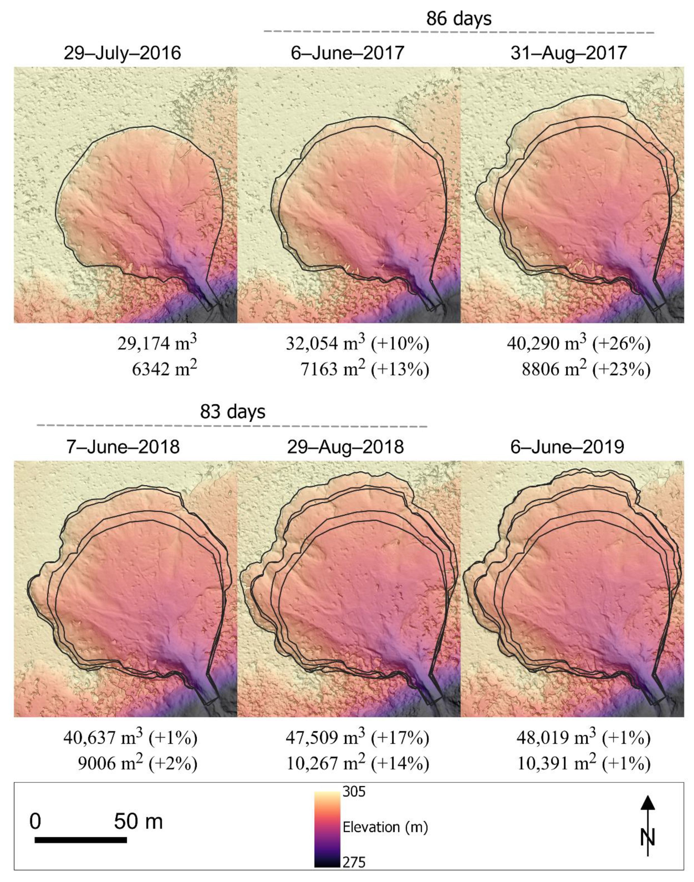
High-resolution remotely sensed data were acquired using RPAS at Slump1 six times during the period 2016–2019 to provide insight of geomorphological properties and change. Monitoring of Slump1 began 29-July-2016, approximately one month following the initial evacuation of sediment from the site. Subsequent RPAS surveys were conducted during 6-June and 31-August of 2017 and 7-June and 29-August 2018. One more survey was conducted during 6-June-2019. Three different RPAS vehicles were used beginning with a 3DR Solo equipped with a GoPro 4 camera during the period 2016–2017, followed by an eBee+ (2018–2019) and DJI Phantom 4 equipped with a FC6310 camera (2019). The flight paths were all pre-programmed using Pix4D Capture for the 3DR Solo, Sensefly eMotion (version 3) for the eBee+, and DJI GS Pro for the DJI Phantom 4. Flight paths were oriented perpendicular to dominant wind direction for each survey. The eBee+ was flown with a (SODA) RGB camera, a (Parrot Sequoia) multisensor, and a (Sensfly ThermoMap) thermal sensor. Thermal imagery was only acquired 6-June-2019. The Sequoia multisensor included a 16-megapixel RGB camera, and 1.2 megapixel green, red, red-edge and near infrared (NIR) bands (spanning average wavelengths of 550, 660, 735, and 790 nm, respectively).
Georeferencing of acquired images required use of ground control points and post-processing kinematic (PPK) corrections. Ground control points (GCPs) were used during the initial flights with the Solo 3DR kit. However, these positions were acquired during 2016 with a simple handheld GPS unit with relatively low accuracy. On the other hand, images acquired during subsequent surveys (June 2017 and 2018–2019) utilized highly accurate differential Global Navigation of Satellite System (GNSS) survey control established using Spectra Precision SP80 receivers and PPK corrections, which can achieve horizontal and vertical accuracies of 3 and 5 mm, respectively. A spatially-accurate orthomosaic generated for June 2017 was used to improve the accuracy of the 2016 and August 2017 RPAS products by using common features (e.g., fallen trees) to establish GCPs. Flight path and photo georeferencing during the Ebee+ RPAS surveys (2018–2019) utilized PPK corrections using SenseFly’s eMotion (version 3) flight processing software. Corrections for the aircraft positions were applied following flights using rinex output from a base station GNSS survey (within 1 km of Slump1), which collected satellite locational information in tandem with the flights. A Spectra Precision (SP80) receiver was used for the base station survey as well as the previous ≥7 h static surveys that were used to derive the control point position. Corrections for the GNSS static survey coordinates were provided by the Natural Resource Canada’s Precise Point Positioning service (https://webapp.geod.nrcan.gc.ca/geod/tools-outils/ppp.php). All images from the 3DR and Ebee+ surveys were processed using Pix4D photogrammetry software (versions 3-4.4.12). All acquired images overlapped by at least 65% to provide sufficient spatial reference points for photogrammetric processing. Shortwave radiance values were recorded using the Sequoia system and used in conjunction with image calibration charts to correct multispectral (green, red, red-edge, and NIR) reflectance values in Pix4D. Corrected multispectral bands were used to generate green, red, red-edge, and NIR reflectance layers. The spatial resolution of the orthomosaics and digital surface models (DSMs) were 3.25 cm for the 3DR/Hero 4 RPAS and 2.90 cm for the Sensfly SODA sensor (Table A1). Reflectance layers generated from the Parrot Sequoia multispectral sensor and SenseFly ThermoMap thermal sensor yielded 12.8 and 18.4 cm pixel resolution, respectively.
The RPAS flight using the Phantom 4 with the FC6310 camera was conducted at a lower altitude (30 m above the top of the slump headwall) to provide higher-resolution mapping data products. The Phantom 4 being used was customized by UAV-Design (Finland) to include GNSS recording capabilities and a spatially-calibrated camera. ReachView flight planning software was used in the field, while Pix4D photogrammetry software was used to generate final mapping products. The Phantom 4 survey also including use of 10 GCPs (five surrounding the slump and five positioned within in the slump) that were corrected using survey control. The spatial resolution of the RGB-derived orthomosaic and DSM was 0.84 cm.

2.2. RPAS Data Analysis

A point cloud of Slump1 and surrounding area was generated using SfM in Pix4D for each sampling interval. The pix4D fill volume tool was used to calculate the cumulative volume of sediment exported from the thaw slump prior to each survey. A polygon extending across the plane of the thaw slump and its entire perimeter provided the elevation reference for determining the volume of space missing from the ground below (i.e., fill volume). An estimation of error was identified for the fill volume of each survey interval using approaches described by Pix4D [34], which assumes that uncertainty is within 1.5 times the grid sample distance (GSD or resolution) volume for each pixel (i.e., 1.5 × GSD3).
A ground irradiance layer was generated, representing the total amount of irradiance (W·m−2) the ground surface was exposed to during daylight hours (10:00 to 18:00 local time). The algorithm was implemented using the r.sun.hourly add-on and r.sun modules for GRASS GIS software (version 7.8.3; [35,36]). The required spatial data layers included the RPAS-derived DSM, and slope and aspect layers, which were generated from the DSM. Other input parameters included date and time range. The timing of summer solstice (20-June-2019) was used to model the most intense irradiance values, when the sun height (vertical solar angle) was greatest.
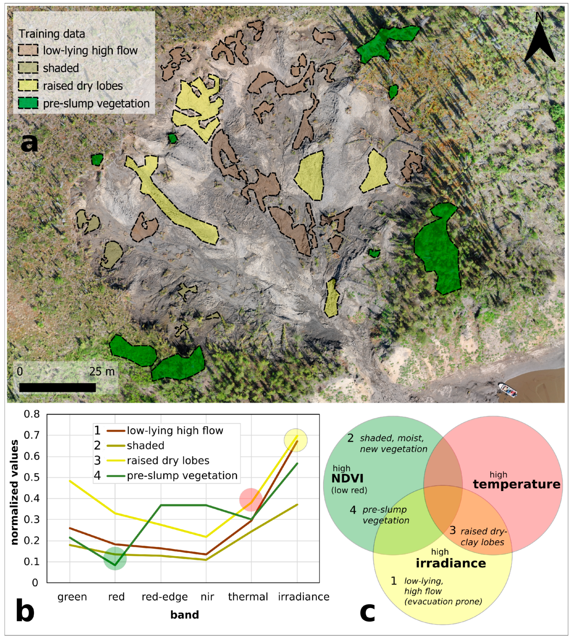
RPAS mapping products were used to explore geomorphological characteristics within Slump1. Differences in vertical profiles and headwall retreat were compared among ten transects that extend from their intersection at the central outflow of Slump1, outward to 5 m past the 2019 headwall. The orientation of the transects were set at 12.5–20° intervals, which correspond with sun azimuth experienced between 6:55 and 17:45 during summer solstice (20-June-2019). The aim was to compare the influence that varying amounts of incident radiation and ground properties (NDVI and temperature) had on thaw slump characteristics and change. For 2019, multispectral (green, red, red-edge and NIR), thermal and irradiance layers were used to classify geomorphological terrain types for Slump1. Maximum likelihood (supervised) classification was used to distinguish terrain types. Pixel training data were identified using the high-resolution (0.84 cm) RPAS-derived orthomosaic and in situ oblique photographs acquired during field campaigns. Accuracy of the supervised classification was evaluated using calculated metrics including overall accuracy, user and producer’s accuracy, kappa statistic, and a confusion matrix output from GRASS GIS [37]. Surface water flow pathways across the varying terrain types were identified using a combination of two terrain modelling procedures and manual digitizing of flow channels visible in the 0.84 cm orthomosaic. The terrain modelling included the topographic water index (TWI), and flow accumulation, both of which were calculated using the DSM for Slump1. TWI was derived using the r.topidx module in GRASS GIS, which utilizes upstream hillslope and area to derive the amount of potential water that drains through each pixel [38,39]. The utility of surface water flow pathway modelling was also explored using the r.flow module for GRASS GIS, which provided a measure of flow accumulation based on density of flowlines passing through each pixel [40].

2.3. Sediment Samples

A total of 40 (thawed) sediment samples were collected from inside Slump1 to characterize physical and chemical properties. During July 2016, six samples were collected along a vertical profile of the northwestern headwall at 10, 60, 80, 100, 120, and 140 cm below the uppermost peat layer horizon. Six more samples were obtained during June 2017 from random locations within low-lying wet areas of the thaw slump floor. During June 2019, samples were collected 10 m apart along three horizontal transects (15 m apart) spanning the floor of Slump1. Sample locations along the transects were recorded using differential GPS. A qualitative assessment of soil moisture (i.e., wet, medium wet, and dry) was recorded at each sampling location along the transects. Approximately 200 cm3 of thawed sediment were collected at each sampling location using cleaned plastic tubing. Once excess sediment was scraped off, the 4 cm tubing sections were capped with minimal air inside, wrapped with plastic film and sealed with tape. Samples were stored at 4 °C until processed at the Water and Environment Lab at Brock University. The samples were analyzed for loss on ignition (LOI), bulk density, gravimetric and volumetric water content, and bulk organic carbon (SOC) and total nitrogen elemental compositions.
Bulk dry soil organic carbon (SOC) and total nitrogen (TN) elemental compositions were measured using methods described by Wolfe et al. [41]. The sediment samples were rinsed with 10% hydrochloric acid to remove carbonates and rinsed repeatedly with de-ionized water until neutral pH returned. Acid-washed samples were freeze-dried to remove moisture and a 500 µm sieve was used to remove coarse organic material. Fine fraction samples (<500 µm) were then analyzed for organic carbon and nitrogen elemental composition using a continuous flow isotope ratio mass spectrometer (CF-IRMS) at the University of Waterloo Environmental Isotope Laboratory.
Relations among sediment analysis results (LOI, dry bulk density, SOC, and TN) and RPAS-derived terrain characteristics were explored to evaluate the influence of thaw slump geomorphological influence on sediment properties. Dry bulk density, SOC, and TN data were also used in conjunction with the cumulative fill (sediment export) volume for each survey interval to estimate SOC and TN mass exported to the debris tongue. The dry bulk density values were converted to mass per unit volume (kg m−3) and multiplied by SOC and TN concentrations. These values were multiplied by Slump1 total fill volume to provide estimates of the cumulative SOC and TN mass exported.

3. Results

3.1. Geomorphology of Slump1

Digital elevation models derived from SfM were used to calculate the total volume of sediment exported at the time of each RPAS survey (Figure 3, Table 1). By 29-July-2016, approximately one month following the initial evacuation of Slump1, a total 29,174 m3 was exported to the debris tongue, where it was available for transport by the Old Crow River. The exported volume and total area grew by 10% and 13%, respectively, by the following spring (6-June-2017). During the next 86 days (until 31-August-2017), Slump1 experienced the greatest volumetric (26%) and areal (23%) increases during this study. This interval was characterized by the warmest temperatures and average rainfall. Increases in thaw slump volume and area were minimal (1% and 2%, respectively) from 31-August-2017 to the following spring (7-June-2018). During the following 83 days (until 29-August-2018), which were characterized by cooler and wetter conditions than during summer 2017, Slump1 experienced a 17% increase in volume and 14% increase in area. The volume and area of Slump1, again, only experienced slight (1%) increases during the next interval up to the final RPAS survey (6-June-2019). The final cumulative volume of sediment exported by this time was 48,019 m3.
The data acquired using RPAS during 6-June-2019 was used to generate several mapping products (DSM, irradiance, NDVI, and thermal), which were used to identify key geomorphological characteristics of Slump1 (Figure 4). The transects within Figure 4 provide a reference of sun altitude (denoted by colour) and azimuth (line direction) during summer solstice when radiative intensity was at maximum potential. The DSM (hillshade) effectively shows the variable relief within the RTS. This is complemented by the total irradiance (11:30–17:30 UTC-7) layer, which identifies zones within the RTS that received high versus low amounts of incident radiation on clear-sky days. These areas were located at the high-relief locations on the RTS floor, and particularly, towards the northern headwall closer to the ends of transects 6 and 7, where ice-wedge cross sections were often observed in the headwall exposure. These transects were also aligned with the sun at peak altitudes (44.7 and 45.5 °C, respectively) during summer solstice. The more shaded areas were situated immediately northwest of raised areas on the RTS floor, and especially, north of the southwest boundary of the RTS. NDVI shows the lack of vegetation across the majority of the RTS. NDVI values were higher where there was vegetation including ‘older’ black spruce trees (with the highest NDVI values) and moss mat, which had been transported toward the central area of the RTS floor during evacuation events. The relatively high NDVI values within the shaded area in the southwest zone highlight newly established graminoids, which were observed for the first time growing during the 6-June-2019 survey. The thermal data are highly variable. Maximum temperatures (up to 48 °C) are along the steep shoreline of the Old Crow River, facing approximately 150° SSW. Other areas with high temperatures are the raised areas in the eastern and northwestern portions of the RTS floor. These areas had high irradiance, although the other central area with high irradiance had relatively lower surface temperatures. The moisture from the thawing northern headwall kept the sediment cool along these low-lying areas that extended from the northern headwall down to the mouth. The shaded area on the south side also had relatively cool temperatures.
Differences in headwall retreat length during the period 2016–2019 (after the initial evacuation had occurred) were compared among 10 transects extending from the central outflow of Slump1 to 5 m outside of the 2019 headwall boundary (Figure 5; Table 2). A transect following the outflow path from the central area (transect 11) is also included in the plot with transect 6. For all ten transects combined, the mean headwall retreat from 29-July-2016 to 6-June-2019 was 17.1 m. The minimum retreat occurred closer to the outflow mouth along SW-NE transects (1, 2, and 10). Greater headwall retreat occurred towards the northwest represented by transects 3, 3.5, and 4, which experienced 17.6, 24.0, and 16.9 m cumulative headwall erosion, respectively. Transects 8–10 are directed to the northeast into an adjacent RTS scar. The greatest retreat during the three-year period was experienced along the northern headwall among transects 5, 6, and 7, which showed 24.9, 27.3 and 29.0 m cumulative headwall erosion length, respectively. Notably, the greatest amount of headwall retreat occurred along transect 7, which aligns with the sun azimuth (181.5°) at the time of maximum sun altitude (45.5° at 14:26 UTC-7; Table 2) during summer solstice (20-June-2019).
RPAS-derived data from 2019 (Figure 4) were evaluated along the profiles (superimposed on RPAS data, e.g., Figure 4a) to compare ground conditions in the directions of varying rates of headwall retreat and sun azimuth and altitudes (Figure 6, Table 2). The majority of Slump1 had no vegetation ground cover as represented by transects 3–8, which have low mean NDVI. The spikes in NDVI along the profiles represent the older vegetation (trees, shrubs and moss mats) that have been transported into the slump during ablation and evacuations. Interestingly, some of this vegetation was relatively healthy during field campaigns (e.g., upright spruce trees) and has potential to re-establish within the RTS scar if evacuations cease. The transects leading to the lateral areas within the southern portion of Slump1 (1, 2, 9 and 10) had the greatest mean NDVI values because of an abundance of older, pre-slump vegetation as well as newly established graminoids. The grasses and mosses present in the stationary sediments among transects 1–3 were observed for the first time during the final survey campaign, almost three years following the initial evacuation. The southwestern area experienced the least amount of headwall retreat and received the greatest amount of shading as shown by the relatively low temperatures and low total irradiance along transects 1 (Figure 4 and Figure 6c,d). There were also relatively low temperatures along the central floor of Slump1 (e.g., along portions of transects 5–7), despite high irradiance (Figure 6d). This area was barren of new vegetation. Field observations indicated that these areas had relatively high moisture supplied from the thawing ice-rich northern headwall. Deep-seated mass wasting was observed along these low-lying corridors immediately following the initial survey (29-July-2016). The sediment with within areas of relatively high ground temperatures (e.g., along transects 4 and 8) had low NDVI, and high irradiance, were dry, and raised (Figure 6a). These raised lobes comprised mostly clay and were less prone to movement.
In summary, the combination of irradiance, multispectral (calibrated green, red, red-edge, and NIR reflectance bands) and thermal data distinguished key geomorphological characteristics within Slump1 (Figure 7), which were observed in the field and were discernable within the high (0.84 cm) resolution orthomosaic. Four classes of interest identified in the field and in the high-resolution RPAS data can be described as (1) low-lying, mixed clay-silt, and barren sediment with high irradiance, low temperature, and prone to mass wasting; (2) headwall-shaded areas with varied relief, cool temperatures and establishment of graminoid and moss vegetation; (3) raised, barren, dry clay lobes, with high irradiance, and temperature; and (4) pre-thaw slump vegetation (e.g., spruce, shrub, grass and moss mat). Figure 7 shows example locations of these terrain classifications identified within Slump1 during the 2019 survey (Figure 7a). The associated normalized spectral signatures of the multispectral, thermal, and irradiance bands within the polygons (Figure 7b) have super-imposed circles identifying the key differences that allow for effective differentiation of the terrain types. The visible and NIR bands were useful for distinguishing all four classes, but mostly for identifying pre-slump vegetation and shaded areas with new vegetation growth (Figure 7b,c). High irradiance values distinguished the open and barren terrain types (classes 1 and 3) from the shaded areas (class 2; yellow circle in Figure 7b,c). Whereas thermal data effectively distinguished the warmer, raised dry clay lobes (class 3) from the cooler, low-lying high flow class 1.
To illustrate further, these RPAS-derived mapping layers from the 2019 survey were used to generate a terrain classification map to highlight the geomorphological differences within Slump1, (Figure 8). The maximum likelihood classification approach was implemented using the training data identified in Figure 7a in GRASS GIS software (version 7.8.3). The overall accuracy of the classification was 98.2%, with a kappa coefficient of 0.97. The most confusion among classes was between shaded, moist areas and the open, moist areas (user accuracy = 90.2%). The other groupings had user and producer accuracies between 97.4 and 99.9%. Terrain classification was attempted for previous years using only RGB and DSM (irradiance) layers with mixed success. While the general areas of the terrain classifications spatially aligned with the 2019 products, user and producer accuracies decreased to as low as 50%. Therefore, the thermal and NIR reflectance data acquired during 2019 provided key layers for differentiating thaw slump geomorphic characteristics.
Surface water flow pathways within Slump1 were identified using the combination of modelling approaches (TWI and flow accumulation) using the DSM and manual digitizing of visible flow channels identified in the 0.84 cm resolution orthomosaic. Based on qualitative comparison of the modelled results with the orthomosaic, TWI (values > 4) provided favorable identification of relatively lower-flow pathways. However, the TWI did not detect much of the larger, incised channels, mostly located in the low-lying areas of the thaw slump. The sensitivity of TWI in these areas was likely reduced because of the effects of shadows within the RPAS-derived images that were used to generate the DSM. Therefore, manually digitized channels (n = 196) were required to enhance identification of the high surface water flow pathways. The flow accumulation model (from the r.flow module in GRASS GIS, version 7.8.3) provided favorable results for identifying the raised ridges. For our application, these mapping layers highlighted differences in low- and high-flow water accumulation among classified thaw slump terrain types (Figure 8). Locations of ridges along the raised dry clay lobes are highlighted in red, which are typically perpendicular to the headwall. Surface water flow pathways (highlighted in blue) represent areas that convey overland water flow and the suspended sediment eroded from fluvial processes. Therefore, many of these high liquid-flow channels are incised into the thaw slump floor.
Degradation and aggradation differences among terrain classification types were compared for each time interval between survey campaigns (Figure 9). The pre-slump vegetation class was not included in the analysis. Headwall degradation (<−2 m), which provided the greatest source of sediment for transport along thaw slump flow paths was also not included since the focus was to compare differences among terrain classes defined within the area of the thaw slump floor. Pixel sampling zones of each class for each survey were identified using the orthomosaic and in situ photographs acquired during the beginning date of each interval. Results were plotted as scaled density for semi-quantitative assessment rather than frequency since variable spatial portions of the terrain type areas were used (Figure 9). Degradation was dominant during the first two intervals up to August 2017 for the three terrain classes (~−0.25–−1.25 m). During this interval, the shaded southwestern zone also experienced some aggradation in spots (<1 m). Aggradation (between 0.2 and 0.9 m) was experienced during fall 2017 to spring 2018, mostly for the low-lying, high-flow accumulation pathways. This sediment was exported during the period June–August 2018. During this interval, similar amounts of erosion occurred within the raised dry clay zones, while less degradation was experienced within the shaded southwest zone. Elevation change was negligible for the three terrain classification types during fall 2018 to spring 2019. Overall, the low-lying, high-flow accumulation pathways experienced the most dynamic elevation changes since these zones received sediment from the headwall as well as the raised dry clay zones. The raised dry clay zones generally degrade over time since there is no sediment source for aggradation. The thawing headwall sediment accumulates within the lower-lying areas that are more prone to evacuation during mass wasting events. The shaded southwest zone was more stabilized than the other terrain types during the last year of this study.

3.2. Thaw Slump Sediment Organic Carbon, and Total Nitrogen

Percent SOC and TN values show variability when grouped by terrain unit classifications (Figure 10, Table A2). Although the number of samples obtained from each terrain grouping are unequal, there are notable distinctions. The greatest differences in SOC and TN concentrations were identified between the shaded areas (with grasses and moss) with the highest values and the raised dry clay lobes with lower values. Twenty-two of the 26 samples from the low-lying, high-flow accumulation zone had SOC values less than the minimum value (1.78%) in the shaded southwest zone. The majority (8/9) of samples from the raised, dry clay lobes also had SOC less than the minimum value from the shaded area. Similarly, TN (%) was typically lower for samples outside of the shaded southwest zone. Thawed sediment sampled from the northwester headwall during July 2016 at 10–140 cm below the ground surface also had relatively low SOC and TN values. Twenty-one of the 26 samples from low-lying, high flow zones and six of the nine samples from raised dry clay zones had TN (%) less than the minimum (0.13%) value in the southwest shaded zone. The low-lying, high-flow accumulation areas had the most variable SOC and TN concentrations since they convey sediment from the other geomorphic zones (headwall, shaded southwest area, and raised dry clay lobes).
More detailed exploration of the relations among terrain and sediment characteristics is shown in Figure A1. Principal components analysis (PCA; Figure A1a) revealed that the higher SOC and TN concentrations in the shaded terrain type was associated with greater slope, NDVI, and bulk density, and lower aspect, temperature, and irradiance. On the other hand, sediment from the raised dry clay lobes was strongly associated with higher aspect, temperature, and irradiance. Samples from the low-lying high flow zones plot between the other terrain classes. Scatterplots of SOC and TN with the other terrain characteristics (Figure A1b) highlight the distinction of the shaded terrain class from the other classification groupings based on individual RPAS-derived datasets. This is most notable for slope, aspect, irradiance and temperature. TWI was not distinguishable among terrain types. There is much more overlap between the low-lying high flow and raised dry clay lobe classifications, especially in terms of nutrient concentrations. However, there is notable distinction in slope and temperature values between these two groupings with the raised dry clay lobes typically being steeper and warmer.
Sediment analysis was coupled with RPAS-derived volume calculations to estimate the total amount of SOC and TN exported as sediment from Slump1 between each sampling interval. Of the 40 sediment samples (Table A2), the 26 samples that were collected within low-lying, high sediment flow (evacuation-prone) areas of the thaw slump were used to calculate mass of SOC and TN export to the debris tongue on the Old Crow River. These samples included 14 from along the 2019 transects and 12 from non-transect locations collected prior to 2019. Median dry bulk density, and median SOC and TN concentrations were 1.293 g cm−3, 1.05% and 0.09%, respectively (Figure 10). SOC and TN storage estimates in the high-flow areas of Slump1 were derived from multiplying bulk density (converted to kg m−3) by SOC and TN concentrations. Median SOC and TN values were 14.9 kg C m−3, and 1.2 kg TN m−3, respectively. After multiplying these values by fill volume values from each RPAS survey, we estimated that Slump1 exported approximately 713 t SOC and 58 t TN to the Old Crow River from the time of initiation during June 2016 to June 2019. Following the initial detachment failure during June 2016, the most SOC (122 t) and TN (10 t) was exported during summer 2017 compared to during 2018 (SOC = 102 t and TN = 8 t).

4. Discussion

This study demonstrates a unique approach that integrates RPAS-derived datasets and in situ measurements for monitoring thaw slump geomorphology, drivers, and influence on soil properties and nutrient mobilization. Discussion of this multifaceted study is broken down among volumetric change monitoring, associated drivers (meteorology, orientation), thaw slump geomorphology, and detected relations with soil nutrients, which can be utilized to refine estimates of downstream impacts. Our findings underscore the dynamic geomorphic properties of permafrost retrogressive thaw slumps that should be considered when anticipating associated impacts on important Arctic and subarctic landscapes such as OCF, that are sensitive to ongoing climate change.
The 2016–2019 time series of high-resolution DSMs produced from SfM provide insight of the seasonal and interannual timing of evacuations. This approach has been performed for many sites across Northwest Territories, Canada, where thaw slumps have reached fill volumes of 3.2 × 10³ to 5.9 × 10⁶ m3 [17]. Slump1 reached a fill volume of 4.8 × 10⁴ m3 by spring 2019, which was 61% greater than its size following the first RPAS survey in July 2016. The (~1-ha) area of Slump1 is relatively large for OCF based on comparison with other thaw slump scars observed in oblique aerial photographs from reconnaissance flights and general assessment of airborne datasets (i.e., AVIRIS-NG). Thaw slump area is much more variable in other landscapes. For example, the median area of thaw slumps across Tuktoyaktuk, NT is 0.4 ha, but reach as large as 5 ha [13].
Volumetric change coupled with analysis of meteorological data provide insight of the drivers of Slump1. While there was greater total accumulated rainfall during 2018, greater evacuation of sediment occurred during the warmer 2017 summer when precipitation was more focused within shorter (2–3 day) time periods during August. These findings are consistent with other studies in northwestern Canada [3,7,13], Alaska [42], and Russia [13], where debris often accumulated on thaw slump floors following headwall erosion and was subsequently exported during precipitation events later in the summer. The high-resolution DSMs produced from RPAS-derived images were ideal for evaluating the timing of steady versus mass-wasting events. However, future studies should attempt more frequent acquisition of high-resolution thaw slump size data to refine insight of meteoric influence on processes driving volumetric change. For example, the timing of RPAS surveys over multiple thaw slumps could be aligned with the frequent (11-day interval) acquisition of TanDEM-X satellite data, which was used by Zwieback et al. [13] for evaluating the timing of thaw slump volumetric change across vast landscapes in northwestern Canada and Russia.
The orientation of thaw slumps can be variable according to local geomorphic properties. While local geomorphic drivers including meteorological conditions and erosion along rivers and coastal areas often represent dominant controls on initial detachment failures, the direction of subsequent maximum headwall retreat and ablation can often be linked with orientation. As noted by Lewkowicz [7], the initiation of thaw slumps on Banks Island were triggered by coastal erosion with high incident radiation on south- and southwest-facing slopes, promoting headwall retreat. Pronounced northward headwall retreat has been observed at other notable sites including the Batagay mega slump in northern Yakutia, Russia [16] and in northwestern Canada [10,17]. Our results are consistent with these observations and highlight the utility of modelled (daily cumulative) irradiance (i.e., during 20-June; summer solstice) for highlighting the importance of orientation in driving greater northward headwall retreat. Other studies have indicated that orientation may be less influential on rates of headwall retreat. For example, Swanson and Nolan [18] noted that the growth of thaw slumps in the Noatak Valley, Alaska was not strongly linked with orientation, particularly with high-irradiance angles, with the greatest headwall retreat rates located along west- and north-facing slopes. This can also be the case for coastal environments, where thaw slump activity is perpetuated strongly by coastal thermo-erosion [15,43]. However, there are many landscapes where the orientation of thaw slump activity may be more effectively predicted when incorporating high-resolution DSM-derived irradiance data. While the orientation of hillslope thaw slumps in the Richardson Mountains-Peel Plateau was predominantly east facing [11] and in the Mackenzie Delta predominantly south and west facing [44], the direction of maximum headwall retreat during years following initiation was not identified. As well, Lewkowicz and Way [14] identified drastic increases in the frequency of thaw slumps on Banks Island, with the highest frequency occurring within the southern portion of the study area. Temperature was identified as an important determinant of this general spatial pattern, although it will be interesting to evaluate the influence of orientation on thaw slump growth rates where remotely sensed data of sufficiently high resolution are available.
Acquisition of high-resolution datasets of thaw slumps at varying stages of development will be useful for predictive spatial modelling of future thaw slump activity and hazard mapping. Preliminary assessment of thaw slump spatial distributions in OCF indicates that orientation is an important geomorphic factor of their formation and development. Thaw slumps predominantly exist here on south- and southeast-facing slopes that experience headward erosion along the steep banks of high-order river channels (i.e., Old Crow River and lower Johnson Creek). Future analyses using high-resolution RPAS-derived data and data acquired during NASA’s Arctic-Boreal Monitoring Experiment Airborne Campaigns (https://above.nasa.gov/airborne_2017.html) will refine our inventory of thaw slump frequency and development patterns.
Multispectral, thermal, and DSM-derived datasets provided refined insight of the complex geomorphology of thaw slumps, which influence their long-term development and influence on biogeochemical cycling. Several studies have utilized SfM with RPAS-derived data to monitor thaw slump geomorphology and volumetric changes in northwestern Canada [17,45,
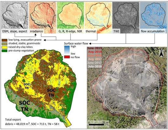
46]. Here, we explored the utility of high-resolution multispectral and thermal datasets for classification of thaw slump terrain types that had varying influence on sediment export and biogeochemical cycling. The most dynamic portion of the Slump1 floor was the low-lying, high-flow accumulation zones, which were readily prone to evacuations during rain events. These low-lying areas received sediment from the thawing headwall and raised dry clay lobes. The raised dry clay lobes were less prone to mobility during mass wasting events but experienced more long-term degradation and weathering as sediment eroded from these areas to the lower-lying high-flow accumulation zone during rain events. The raised dry clay lobes comprised clay sediment that were thawed longer than most of the sediment being conveyed seasonally along the low-lying high-flow accumulation zone. The more shaded zone in the southwest area experienced stabilized conditions relatively early, and as a result, saw recent growth of moss and graminoid vegetation. The low-lying, high sediment flow terrain zones were differentiated from the raised dry clay lobes based on temperature and slope. The raised dry clay lobes had high temperature since they were out of the flow pathway of headwall meltwater and, with greater slope, also have more efficient drainage than the low-lying high flow zones. The shaded zone with new vegetation, which also had cooler temperatures, could be distinguished with its unique combination of (green to NIR) spectral signatures and low cumulative daily irradiance.
Past studies have identified the role of fluvial erosion transporting sediment from thaw slumps e.g., [3,38]. Incised channels, formed from fluvial erosion, were observed during field campaigns in Slump1, which at times, directed sediment-laden water to the Old Crow River. Depending on the intensity and duration of rainfall events and ground ice meltwater volumes, effective drainage of runoff along these conduits reduced pooling and supersaturation that may have otherwise promoted deep seated mass wasting. Surface water channels were easily identifiable within the high-resolution orthomosaic. Other flow pathways that were more difficult to visualize and document were effectively modelled using the TWI derived from the DSM. For example, sheetflood pathways, that form alluvial fans at the base of the headwall [8], were effectively identified with TWI (values > 4) and connected with visibly incised channels. Flow accumulation analysis [40] also identified low or non-flow ridges that were less prone to being exported during mass wasting. While shadows can hamper the detection of higher-order incised channels, these high-resolution optical multispectral datasets can provide key insight of the fluvial processes influencing thaw slump development and influence on downstream environments.
At landscape and regional scales, the sediments exposed and mobilized by individual thaw slumps are often characterized by a homogeneous nutrient (i.e., SOC) supply, which varies according to broad regional soil types e.g., [30]. Obu et al. [31] did find that differences in SOC and TN concentrations were associated with feature types including mass-wasting disturbance (i.e., thaw slumps), peat, and fluvial deposits, as well as terrain characteristics including slope angle and TWI. For instance, SOC and TN was found to be positively correlated with TWI, negatively correlated with slope angle and of lower concentrations in the upper sediments of thaw slumps relative to other landscape features. Findings presented here suggest that the influence of slope angle and TWI on SOC and TN can be overshadowed at finer scales by physiographic properties within individual thaw slumps. We detected differences in SOC and TN concentrations among the terrain classifications in Slump1 with the shaded areas having higher values, despite having steeper slope angles. The retention of soil moisture within the shaded area of Slump1 provided ideal microenvironment for establishment of mosses and graminoids, which allowed for accumulation of organic matter. This was contrary to the low nutrient values found in the non-shaded areas that were raised and aligned with the highest incident radiation. These dry clay lobes slowly degraded during this study but retained sediment that had been exposed to the most weathering. Therefore, low SOC and TN are likely in response to leaching downslope, which is consistent with Obu et al. [31]. SOC and TN values from the low-lying high-flow accumulation zones were the most variable since sediment from the other terrain classification zones were mixed and transported along these pathways. Because mixing of sediments occurs during evacuation events, we can expect that outflow sediment nutrient concentrations to be proportional to the size and relative contribution of the source geomorphic terrain types.
The SOC and TN results (14.9 kg C m−3 and 1.2 kg TN m−3, respectively) used in our nutrient flux calculations are less than those found by Obu et al. [31] on Herschel Island, Yukon, Canada who reported thaw slumps to have 20.9 kg C m−3, and 3.7 kg TN m−3, respectively, based on core samples. They suggest that the nutrient concentrations were higher at their sites, below 50 cm from the surface, because of greater aeration and microbial activity at the surface [47] and subsequent carbon degradation [48]. This may also be the case for our surface samples from the raised dry clay lobes in Slump1. However, the six samples obtained along a vertical profile (from 10 to 140 cm below surface) at the headwall of Slump1 had similar dry bulk density, SOC, and TN values as the other zones of the thaw slump floor. The consistency of these values suggests that our SOC and TN flux measurements are representative of sediment being exported during mass wasting events. These values are also consistent with results from the North Slope of Alaska [49]. However, additional sediment sample analysis of thaw slumps in OCF should be completed to ensure our calculations are not conservative.
High-resolution terrain classification mapping of thaw slumps using thermal, multispectral and elevation datasets provides useful context when interpreting thaw slump nutrient flux and biogeochemical cycling. Consideration of within-region variation in thermokarst intensity and landscape properties is critical for determining biogeochemical responses [23,25]. Ongoing research should continue to maximize the use of high-resolution elevation, multispectral, and thermal datasets within situ measurements of sediment and downstream properties to build our knowledge of thaw slump biogeochemical cycling and associated impacts on aquatic environments. Widespread high-resolution mapping and analyses can provide much needed context to strengthen estimates of carbon stocks [30], carbon atmospheric flux [27], and carbon mobility projections based on the varying mitigation strategies [50].

5. Conclusions

This study showcases the utility of RPAS datasets for monitoring the activity and geomorphological characteristics of permafrost retrogressive thaw slumps. Furthermore, findings comprise key insight into the processes driving thaw slump development and relations among geomorphic and sediment nutrient compositions. Integrated datasets were used to estimate sediment load and SOC and TN load volumes exported to the Old Crow River between each survey interval during the three-year study.
Structure-from-motion analysis of RPAS-derived RGB photographs provided key information of retrogressive thaw slump geomorphic properties and change in response to meteorological drivers. RPAS surveys revealed that 29,174 m3 of sediment was exported during the initial detachment failure with subsequent evacuations exporting an additional 18,845 m3 until June 2019. Greater sediment export occurred during the warmer and drier summer 2017 (8236 m3) compared to summer 2018 (6872 m3). However, the fewer rain events during August 2017 were of higher intensity and concentrated within shorter time intervals compared to the rain events more evenly distributed during 2018. The northern headwall experienced the greatest amount of retreat owing to its alignment with the highest incident radiation and the ablation of ice wedges that were commonly observed along its face (Figure 4). More intense incident radiation during the warmer summer 2017 accounts for greater headwall retreat and subsequent evacuations, which was enhanced during August rain events. The north-south alignment of the maximum direction of thaw slump headwall retreat showcases the importance of incident radiation on the detected volumetric change. Modelled (summer solstice) cumulative daily solar irradiance (generated from a DSM) is highly useful for explaining anticipating headwall retreat properties.
Combined RPAS-derived irradiance, multispectral and thermal data provided key insight of thaw slump geomorphology. Maximum likelihood supervised classification using these layers provided high-resolution mapping of thaw slump terrain types including (1) low-lying, high-flow accumulation, evacuation-prone sediment; (2) shaded areas with graminoid and moss vegetation; (3) raised, dry clay lobes; and (4) pre-thaw slump vegetation (e.g., spruce, shrub, grass, and moss mat).
Surface water runoff pathways within a thaw slump can be detected using combined modelling and manual visual identification approaches. Small, low-order channels (formed from pluvial and rill erosion) and sheetflood pathways can be readily identified with modelling (e.g., TWI). However, this approach is less effective for highlighting larger channels covered by shadows during the RPAS surveys. On the other hand, these higher-order channels are easily distinguishable with high-resolution (0.84 cm) RGB imagery and can be manually digitized.
SOC and TN concentrations varied among classified terrain types with the highest concentrations within the shaded areas with steeper slope values where new vegetation had established, and the lowest concentrations in the raised dry clay lobes that were subjected to prolonged weathering. The low-lying, high-accumulation zone had the most variable concentrations since these areas conveyed sediment from the other two classes. Coupled RPAS-derived volume, sediment dry bulk density and SOC and TN data indicated that Slump1 exported approximately 713 t SOC and 58 t TN during the three-year study. The most SOC (122 t) and TN (10 t) was exported during summer 2017 compared to during 2018 (Corg = 102 t and TN = 8 t).

Author Contributions

Conceptualization, K.W.T.; methodology, K.W.T.; software, K.W.T.; validation, K.W.T.; formal analysis, K.W.T., M.D.P., D.D.H.; investigation, K.W.T., M.D.P., D.D.H.; resources, K.W.T.; data curation, K.W.T., M.D.P., D.D.H.; writing—original draft preparation, K.W.T.; writing—review and editing, K.W.T., M.D.P., D.D.H.; visualization, K.W.T.; supervision, K.W.T.; project administration, K.W.T.; funding acquisition, K.W.T., M.D.P., D.D.H. All authors have read and agreed to the published version of the manuscript.

Funding

This research was funded by the Natural Sciences and Engineering Research Council of Canada’s Discovery Grant and Northern Supplement programs (grant number 2016-4286 and 477155, respectively), Polar Knowledge Canada (grant number NST-1718-0017), Polar Continental Shelf Program (Project numbers 64316, 67817, and 67518), Canada’s Foundation of Innovation John R. Evans Leaders Fund (grant number 36803), and the Northern Scientific Training Program.

Data Availability Statement

Data presented in this study are available in the Appendix A of this article.

Acknowledgments

The authors would like to thank the community of Old Crow and the Vuntut Gwitchin Government for facilitating this research project. In particular, we would like to thank Dougie Charlie, Clifton Nagwan, Robert Kyikavichik, James Linklater, Danny Kassi and Caleb Charlie for their knowledge and guidance when working in their traditional territory. We are also thankful to Megan Williams who provided much needed logistical planning support. Brent Thorne and Luke Gray also provided much needed assistance with fieldwork during 2017–2018. We would like to thank Duane Froese and Brent Wolfe for their informative reviews of the manuscript.

Conflicts of Interest

The authors declare no conflict of interest.

Appendix A

Table A1. Details of RPAS photo acquisition and photogrammetry processing results.
DatePlatformSensorSurvey Area (ha)Number of ImagesResolution of Output Layer (s) (cm)Mean Point Cloud Density (per m3)
29-July-20163DR SoloGoPro 46.751443.25114.47
6-June-20173DR SoloGoPro 411.152783.25197.84
31-August-20173DR SoloGoPro 411.041563.6796.45
7-June-2018eBee+SODA53.993232.901448.07
29-August-2018eBee+SODA53.793422.91940.24
6-June-2019eBee+SODA116.444913.00334.12
Sequoia132.12488/band12.77N/A
Thermo Map137.68356118.43N/A
DJI Phantom 4Phantom (FC6310 RGB)2.454100.845572.43
Table A2. Sediment chemistry and RPAS data values for samples and sample locations. RPAS multispectral (green, red, re-edge, and near infrared) reflectance data and DSM-derivative (slope and aspect) data are represented by majority (modal) pixel values within 1 m radius zones around the transect points (n = 28) sampled during 6-June-2019. Terrain ID values represent low-lying high flow (1), shaded with new vegetation (2), and raised open dry clay lobes (3).
Sample IDSample DateDry Bulk Density
(g/cm3)
SOC
(%)
TN (%)Terrain IDSlopeAspectIrradiance
(W m−2)
GreenRedRed-EdgeNIRThermal
(°C)
SED16 June 20190.8711.9800.173216.38345.01365.8040.06100.06990.07860.090315.785
SED26 June 20191.1891.8300.12820.62545.02065.3710.05800.06520.07780.094315.644
SED36 June 20190.5580.9100.08531.171315.04252.250.08210.08990.09510.111419.839
SED46 June 20190.7281.1000.090311.735360.03550.7990.10460.12040.12030.138217.745
SED56 June 20190.7950.9900.09112.890360.03919.6990.06870.07520.08010.098116.955
SED66 June 20191.2401.4300.13310.000270.04246.1060.05910.05950.06750.086918.514
SED76 June 20191.0761.3100.11417.479315.04414.6960.06120.06930.08570.106917.918
SED86 June 20191.0890.7900.07210.103270.04400.130.05500.06130.07670.091118.856
SED96 June 20191.1000.7700.07015.030251.64688.1970.08260.09860.12190.135220.591
SED106 June 20191.1710.8900.08135.622135.01683.7980.04860.05640.06400.076613.393
SED116 June 20191.0633.2400.215220.15890.02945.1240.05110.05680.07230.094513.465
SED126 June 20191.2491.7800.153215.51645.01945.9840.04190.03870.05320.073214.755
SED136 June 20191.2351.5500.11113.656315.03700.0760.05840.06410.07390.087916.513
SED146 June 20191.1421.5100.137310.666296.73412.7570.08930.10260.11320.126819.397
SED156 June 20191.2221.5800.14813.276315.04180.1910.07760.08540.09270.108117.732
SED166 June 20191.3122.4500.16910.000315.04245.8790.06890.07530.09500.107717.491
SED176 June 20191.1561.0000.08533.280315.03327.6820.06070.06860.07630.087119.482
SED186 June 20191.0741.6000.13631.045225.05019.7890.09140.10400.11490.128620.005
SED196 June 20191.1771.4300.11537.242315.04416.4110.08500.11130.11780.132721.317
SED206 June 20191.2001.2400.09611.397225.03666.5320.05660.06890.08030.095718.215
SED216 June 20190.9681.9000.12712.093270.04233.4870.04950.05620.07630.097722.304
SED226 June 20191.1832.9600.181212.83245.0405.60730.03650.03210.04740.063614.379
SED236 June 20191.2830.9600.08610.640315.03334.0050.06660.06950.08360.098015.444
SED246 June 20190.8081.7000.127314.883315.04886.8980.07990.08730.09880.119819.672
SED256 June 20191.1431.8600.18215.843270.04527.9660.06330.06820.07640.089015.073
SED266 June 20191.2640.4700.04510.0000.04245.7560.06920.07500.08980.104712.915
SED276 June 20191.2861.5600.12410.478225.04271.7710.03090.02220.03200.042818.681
SED286 June 20191.1581.8100.135312.537270.04204.5560.10230.12440.14290.157120.549
exposure_10cm29 July 20161.6060.9550.0631
exposure_60cm29 July 20161.5850.7810.0701
exposure_80cm29 July 20161.4570.6240.0601
exposure_100cm29 July 20161.4710.7610.0701
exposure_120cm29 July 20161.6040.8500.0731
exposure_140cm29 July 20161.5060.7940.0651
west17 June 20171.4740.9920.0811
south17 June 20171.5970.9210.0761
south27 June 20171.4621.5870.1221
west27 June 20171.3771.1390.0781
south37 June 20171.4741.1060.0931
unsure7 June 20171.2992.4960.1611
Figure A1. Relations detected among terrain and soil properties presented in (a) a PCA with eigenvectors representing terrain characteristics, which account for 57.9% of variability (PC1 = 38.8% and PC2 = 19.1%) among transect samples. Bulk density, loss-on-ignition (LOI), SOC and N values were derived from sediment samples, while the other terrain characteristics are the majority (modal) pixel values of each associated RPAS-derived mapping layer within 1 m of sampling sites. Score colours are grouped by the terrain classification that the sample sites were within. The importance of RPAS-derived terrain characteristics on SOC and N concentrations are explored in (b) scatterplots, which also have point colours grouped by terrain classification. Ellipses superimposed on scatterplots assume a multivariate t distribution for each terrain class.
Remotesensing 13 00171 g0a1

References

  1. Lantz, T.C.; Kokelj, S.V. Increasing rates of retrogressive thaw slump activity in the Mackenzie Delta region, NWT, Canada. Geophys. Res. Lett. 2008, 35, L06502. [Google Scholar] [CrossRef]
  2. Kokelj, S.V.; Jorgenson, M.T. Advances in Thermokarst Research. Permafr. Periglac. Process. 2013, 24, 108–119. [Google Scholar] [CrossRef]
  3. Kokelj, S.V.; Tunnicliffe, J.; Lacelle, D.; Lantz, T.C.; Chin, K.S.; Fraser, R.H. Increased precipitation drives mega slump development and destabilization of ice-rich permafrost terrain, northwestern Canada. Glob. Planet. Chang. 2015, 129, 56–68. [Google Scholar] [CrossRef] [Green Version]
  4. Segal, R.A.; Lantz, T.C.; Kokelj, S.V. Acceleration of thaw slump activity in glaciated landscapes of the Western Canadian Arctic. Environ. Res. Lett. 2016, 11, 034025. [Google Scholar] [CrossRef]
  5. Burn, C.R.; Lewkowicz, A.G. Retrogressive thaw slumps. Can. Geogr. 1990, 34, 273–276. [Google Scholar] [CrossRef]
  6. Lantuit, H.; Pollard, W.H. Fifty years of coastal erosion and retrogressive thaw slump activity on Herschel Island, southern Beaufort Sea, Yukon Territory, Canada. Geomorphology 2008, 95, 84–102. [Google Scholar] [CrossRef]
  7. Lewkowicz, A.G. Headwall retreat of ground-ice slumps, Banks Island, Northwest Territories. Can. J. Earth Sci. 1987, 24, 1077–1085. [Google Scholar] [CrossRef]
  8. Murton, J.B. Thermokarst sediments and sedimentary structures, Tuktoyaktuk Coastlands, western Arctic Canada. Glob. Planet. Chang. 2001, 28, 175–192. [Google Scholar] [CrossRef]
  9. Lacelle, D.; Bjornson, J.; Lauriol, B. Climatic and geomorphic factors affecting contemporary (1950–2004) activity of retrogressive thaw slumps on the Aklavik Plateau, Richardson Mountains, NWT, Canada. Permafr. Periglac. Process. 2010, 21, 1–15. [Google Scholar] [CrossRef]
  10. Lantuit, H.; Pollard, W.H.; Couture, N.; Fritz, M.; Schirrmeister, L.; Meyer, H.; Hubberten, H. Modern and Late Holocene Retrogressive Thaw Slump Activity on the Yukon Coastal Plain and Herschel Island, Yukon Territory, Canada. Permafr. Periglac. Process. 2012, 23, 39–51. [Google Scholar] [CrossRef]
  11. Lacelle, D.; Brooker, A.; Fraser, R.H.; Kokelj, S.V. Distribution and growth of thaw slumps in the Richardson Mountains–Peel Plateau region, northwestern Canada. Geomorphology 2015, 235, 40–51. [Google Scholar] [CrossRef]
  12. Luo, J.; Niu, F.; Lin, Z.; Liu, M.; Yin, G. Recent acceleration of thaw slumping in permafrost terrain of Qinghai-Tibet Plateau: An example from the Beiluhe Region. Geomorphology 2019, 341, 79–85. [Google Scholar] [CrossRef]
  13. Zwieback, S.; Kokelj, S.V.; Günther, F.; Boike, J.; Grosse, G.; Hajnsek, I. Sub-seasonal thaw slump mass wasting is not consistently energy limited at the landscape scale. Cryosphere 2018, 12, 549–564. [Google Scholar] [CrossRef] [Green Version]
  14. Lewkowicz, A.G.; Way, R.G. Extremes of summer climate trigger thousands of thermokarst landslides in a High Arctic environment. Nat. Commun. 2019, 10, 1329. [Google Scholar] [CrossRef] [Green Version]
  15. Günther, F.; Overduin, P.P.; Sandakov, A.V.; Grosse, G.; Grigoriev, M.N. Short- and long-term thermo-erosion of ice-rich permafrost coasts in the Laptev Sea region. Biogeosciences 2013, 10, 4297–4318. [Google Scholar] [CrossRef] [Green Version]
  16. Vadakkedath, V.; Zawadzki, J.; Przeździecki, K. Multisensory satellite observations of the expansion of the Batagaika crater and succession of vegetation in its interior from 1991 to 2018. Environ. Earth Sci. 2020, 79, 150. [Google Scholar] [CrossRef] [Green Version]
  17. van der Sluijs, J.; Kokelj, S.V.; Fraser, R.H.; Tunnicliffe, J.; Lacelle, D. Permafrost Terrain Dynamics and Infrastructure Impacts Revealed by UAV Photogrammetry and Thermal Imaging. Remote Sens. 2018, 10, 1734. [Google Scholar] [CrossRef] [Green Version]
  18. Swanson, D.K.; Nolan, M. Growth of retrogressive thaw slumps in the Noatak Valley, Alaska, 2010–2016, measured by airborne photogrammetry. Remote Sens. 2018, 10, 983. [Google Scholar] [CrossRef] [Green Version]
  19. Mesquita, P.S.; Wrona, F.J.; Prowse, T.D. Effects of retrogressive permafrost thaw slumping on sediment chemistry and submerged macrophytes in Arctic tundra lakes. Freshw. Biol. 2010, 55, 2347–2358. [Google Scholar] [CrossRef]
  20. Moquin, P.A.; Wrona, F.J. Effects of permafrost degradation on water and sediment quality and heterotrophic bacterial production of Arctic tundra lakes: An experimental approach. Limnol. Oceanogr. 2015, 60, 1484–1497. [Google Scholar] [CrossRef]
  21. Thienpont, J.R.; Rühland, K.M.; Pisaric, M.F.J.; Kokelj, S.V.; Kimpe, L.E.; Blais, J.M.; Smol, J.P. Biological responses to permafrost thaw slumping in Canadian Arctic lakes: Aquatic biota response to permafrost thaw. Freshw. Biol. 2013, 58, 337–353. [Google Scholar] [CrossRef]
  22. Frey, K.E.; McClelland, J.W. Impacts of permafrost degradation on arctic river biogeochemistry. Hydrol. Process. 2009, 23, 169–182. [Google Scholar] [CrossRef]
  23. Littlefair, C.A.; Tank, S.E.; Kokelj, S.V. Retrogressive thaw slumps temper dissolved organic carbon delivery to streams of the Peel Plateau, NWT, Canada. Biogeosciences 2017, 14, 5487–5505. [Google Scholar] [CrossRef] [Green Version]
  24. Kendrick, M.R.; Huryn, A.D.; Bowden, W.B.; Deegan, L.A.; Findlay, R.H.; Hershey, A.E.; Peterson, B.J.; Beneš, J.P.; Schuett, E.B. Linking permafrost thaw to shifting biogeochemistry and food web resources in an arctic river. Glob. Chang. Biol. 2018, 24, 5738–5750. [Google Scholar] [CrossRef] [PubMed]
  25. Tank, S.E.; Vonk, J.E.; Walvoord, M.A.; McClelland, J.W.; Laurion, I.; Abbott, B.W. Landscape matters: Predicting the biogeochemical effects of permafrost thaw on aquatic networks with a state factor approach. Permafr. Periglac. Process. 2020, 31, 358–370. [Google Scholar] [CrossRef]
  26. Lafrenière, M.J.; Lamoureux, S.F. Effects of changing permafrost conditions on hydrological processes and fluvial fluxes. Earth-Sci. Rev. 2019, 191, 212–223. [Google Scholar] [CrossRef]
  27. Schuur, E.; McGuire, A.; Schädel, C.; Grosse, G.; Harden, J.; Hayes, D.; Hugelius, G.; Koven, C.; Kuhry, P.; Lawrence, D.; et al. Climate change and the permafrost carbon feedback. Nature 2015, 520, 171–179. [Google Scholar] [CrossRef]
  28. Strauss, J.; Schirrmeister, L.; Grosse, G.; Fortier, D.; Hugelius, G.; Knoblauch, C.; Romanovsky, V.; Schädel, C.; von Deimling, T.S.; Schuur, E.A.G.; et al. Deep Yedoma permafrost: A synthesis of depositional characteristics and carbon vulnerability. Earth-Sci. Rev. 2017, 172, 75–86. [Google Scholar] [CrossRef] [Green Version]
  29. Schuur, E.A.G.; Abbott, B. Climate change: High risk of permafrost thaw. Nature (Comment) 2011, 480, 32–33. [Google Scholar] [CrossRef]
  30. Hugelius, G.; Strauss, J.; Zubrzycki, S.; Harden, J.W.; Schuur, E.A.G.; Ping, C.-L.; Schirrmeister, L.; Grosse, G.; Michaelson, G.J.; Koven, C.D.; et al. Estimated stocks of circumpolar permafrost carbon with quantified uncertainty ranges and identified data gaps. Biogeosciences 2014, 11, 6573–6593. [Google Scholar] [CrossRef] [Green Version]
  31. Obu, J.; Lantuit, H.; Myers-Smith, I.; Heim, B.; Wolter, J.; Fritz, M. Effect of Terrain Characteristics on Soil Organic Carbon and Total Nitrogen Stocks in Soils of Herschel Island, Western Canadian Arctic. Permafr. Periglac. Process. 2015, 28, 92–107. [Google Scholar] [CrossRef] [Green Version]
  32. Vonk, J.E.; Tank, S.E.; Walvoord, M.A. Integrating hydrology and biogeochemistry across frozen landscapes. Nat. Commun. 2019, 10, 5377. [Google Scholar] [CrossRef] [PubMed] [Green Version]
  33. Lauriol, B.; Duguay, C.R.; Riel, A. Response of the Porcupine and Old Crow rivers in northern Yukon, Canada, to Holocene climatic change. Holocene 2002, 12, 1. [Google Scholar] [CrossRef]
  34. Pix4D. Error Estimation in Volume Calculation. Available online: https://support.pix4d.com/hc/en-us/articles/202559219-Error-estimation-in-volume-calculation (accessed on 24 December 2020).
  35. Petras, V.; Petrasova, A. GRASS GIS r.Sun.Daily Add-on Module. (Updated 2020). NCSU GeoForAll Lab, North Carolina State University, Center for Geospatial Analytics in Raleigh, NC, USA. Available online: https://grass.osgeo.org/grass78/manuals/addons/r.sun.hourly.html (accessed on 4 June 2020).
  36. Hofierka, J.; Marcel, S. GRASS GIS r.Sun Manual. (Updated 2020). GeoModel, Bratislava, Slovakia. Available online: https://grass.osgeo.org/grass78/manuals/r.sun.html (accessed on 4 June 2020).
  37. Wen, T. GRASS GIS r.Kappa Add-on Manual. (Updated 2020). University of Illinois at Urbana-Champaign, Illinois. Available online: https://grass.osgeo.org/grass78/manuals/r.kappa.html (accessed on 4 June 2020).
  38. Cho, H. GIS Hydrological Modeling System by Using Programming Interface of GRASS. Master’s Thesis, Kyungpook National University, Daegu, Korea, 2000. [Google Scholar]
  39. Moore, I.D.; Grayson, R.B.; Ladson, A.R. Digital Terrain Modelling: A Review of Hydrological, Geomorphological, and Biological Applications. Hydrol. Process. 1991, 5, 3–30. [Google Scholar] [CrossRef]
  40. Caplan, J.; Ruesink, M.; Mitášová, H. GRASS GIS r.Flow Add-on Manual. (Updated 2019). University of Illinois at Urbana-Champaign. Available online: https://grass.osgeo.org/grass79/manuals/r.flow.html (accessed on 4 June 2020).
  41. Wolfe, B.B.; Edwards, T.W.D.; Elgood, R.J.; Beuning, K.R.M. Carbon and oxygen isotope analysis of lake sediment cellulose: Methods and applications. In Tracking Environmental Change in Lake Sediments: Physical and Geochemical Methods; Last, W.M., Smol, J.P., Eds.; Kluwer Academic Press: Dordrecht, The Netherlands, 2001; Volume 2, pp. 373–400. [Google Scholar]
  42. Balser, A.W.; Jones, J.B.; Gens, R. Timing of retrogressive thaw slump initiation in the Noatak Basin, northwest Alaska, USA. J. Geophys. Res. Earth Surf. 2014, 119, 1106–1120. [Google Scholar] [CrossRef]
  43. Obu, J.; Lantuit, H.; Fritz, M.; Pollard, W.H.; Sachs, T.; Günther, F. Relation between planimetric and volumetric measurements of permafrost coast erosion: A case study from Herschel Island, western Canadian Arctic. Polar. Res. 2016, 35, 30313. [Google Scholar] [CrossRef] [Green Version]
  44. Kokelj, S.V.; Lantz, T.C.; Kanigan, J.; Smith, S.L.; Coutts, R. Origin and polycyclic behaviour of tundra thaw slumps, Mackenzie Delta region, Northwest Territories, Canada. Permafr. Periglac. Process. 2009, 20, 173–184. [Google Scholar] [CrossRef]
  45. Fraser, R.H.; Olthof, I.; Maloley, M.; Fernandes, R.; Prevost, C.; van der Sluijs, J. UAV photogrammetry for mapping and monitoring of northern permafrost landscapes. Int. Arch. Photogramm. Remote Sens. Spat. Inf. Sci. 2015, 1, 361. [Google Scholar] [CrossRef] [Green Version]
  46. Armstrong, L.; Lacelle, D.; Fraser, R.H.; Kokelj, S.; Knudby, A. Thaw slump activity measured using stationary cameras in time-lapse and Structure-from-Motion photogrammetry. Arct. Sci. 2018, 4, 827–845. [Google Scholar] [CrossRef]
  47. Pautler, B.G.; Simpson, A.J.; Mcnally, D.J.; Lamoureux, S.F.; Simpson, M.J. Arctic Permafrost Active Layer Detachments Stimulate Microbial Activity and Degradation of Soil Organic Matter. Environ. Sci. Technol. 2010, 44, 4076–4082. [Google Scholar] [CrossRef] [PubMed]
  48. Koven, C.D.; Ringeval, B.; Friedlingstein, P.; Ciais, P.; Cadule, P.; Khvorostyanov, D.; Krinner, G.; Tarnocai, C. Permafrost carbon-climate feedbacks accelerate global warming. Proc. Natl. Acad. Sci. USA 2011, 108, 14769–14774. [Google Scholar] [CrossRef] [PubMed] [Green Version]
  49. Abbott, B.W.; Jones, J.B. Permafrost collapse alters soil carbon stocks, respiration, CH4, and N2O in upland tundra. Glob. Chang. Biol. 2015, 21, 4570–4587. [Google Scholar] [CrossRef] [PubMed]
  50. McGuire, A.; Lawrence, D.M.; Koven, C.; Clein, J.S.; Burke, E.; Chen, G.; Jafarov, E.; MacDougall, A.H.; Marchenko, S.; Nicolsky, D.; et al. Dependence of the evolution of carbon dynamics in the northern permafrost region on the trajectory of climate change. Proc. Natl. Acad. Sci. USA 2018, 115, 3882–3887. [Google Scholar] [CrossRef] [PubMed] [Green Version]
Figure 1. Site map of Slump1 within (a) Old Crow Flats, northern Yukon, Canada. The spatial extent of Slump1 relative to the Old Crow River and surrounding features (e.g., debris tongue and thaw slump scars are shown in (b) an orthomosaic (acquired 6-June-2019) and (c) oblique photograph (acquired 29 July 2016). An example of an ice-wedge cross section observed along the northern headwall is shown in (d).
Remotesensing 13 00171 g001
Figure 2. Meteorological conditions experienced during this study with (a) daily precipitation values represented in the bar plot and the 7-day running mean temperature represented as the blue line. Daily precipitation is also shown (b) grouped by month. Boxes represent the interquartile range (IQR) below the 75% quantile for each month. Median daily cumulative precipitation for each month is shown as a line inside each box. Whiskers extend to the greatest value equal to 1.5 × IQR above the 75% quantile. Points above whiskers are statistical outliers. Orange arrows highlight the timing of six RPAS surveys conducted during this study.
Remotesensing 13 00171 g002
Figure 3. Time series of change in Slump1 during the period 2016–2019. Total volume and percent volume change for each interval is listed under each map. Elevation maps comprise two DSM layers that include a continuous colour (60% opacity) layer superimposed on a hillshade layer (solar altitude = 40°, azimuth = 210°).
Remotesensing 13 00171 g003
Figure 4. Mapping products generated from RPAS surveys conducted during this study including the (a) DSM, (b) total irradiance during summer solstice (11:30–17:30 UTC-7), (c) NDVI, and (d) thermal (°C). The colour of the superimposed transects correspond with sun altitude when the transects are aligned with the sun azimuth at the corresponding time of day. Dark brown represents low sun altitude earlier in the day, while yellow represents high sun altitude during the late afternoon. Blue points represent the locations where and when ice wedges were observed within the headwall exposure.
Remotesensing 13 00171 g004
Figure 5. Elevation profiles along transects extending from the central outflow of Slump1.
Remotesensing 13 00171 g005
Figure 6. Comparison of (June 2019) profiles of RPAS-derived (a) elevation, (b) NDVI, (c) ground temperature, and (d) total irradiance during peak sun hours (11:30–17:30 UTC-7). Line colours are grouped by sun altitude, with darker colours being relatively earlier or later in the day versus lighter yellow representing profiles aligned with the sun at peak midday hours.
Remotesensing 13 00171 g006
Figure 7. (a) Locations of terrain classes from the 2019 RPAS survey with (b) associated spectral signatures spanning normalized multispectral, thermal and DSM-derived irradiance bands. The key points of spectral separation (highlighted by the small circles) are further explained in the (c) Venn diagram, where circles represent generalized (high) band values and combinations that effectivity distinguish the (numbered) terrain classes.
Remotesensing 13 00171 g007
Figure 8. Maps showing results from the maximum likelihood classification and flow detection of Slump1, which highlight distinct geomorphological properties. Surface water flow pathways determined from modeled (TWI) and manual digitizing are shown in blue. The red areas were identified from flow modeling as areas of no-flow accumulation and were identified in the field and in RPAS-derived mapping products as ridges along the raised dry-clay lobes. Oblique photographs (lower left) of relatively shaded area show newly established graminoids and mosses. Black circles are locations where sediment was sampled during June 2019.
Remotesensing 13 00171 g008
Figure 9. Scaled density of elevation change within each terrain class and between each sampling interval. Degradation and aggradation are compared for each terrain class, which were identified using the corresponding orthomosaics and in situ photographs from the beginning of each interval.
Remotesensing 13 00171 g009
Figure 10. Comparison of thaw slump sediment (a) dry bulk density (g cm−3), (b) SOC (%), and (c) TN (%). Points are separated along the x axes based on thaw slump terrain classes. Point colours represent the qualitative description of sediment moisture. Values derived for the period 2016–2017 were grouped within the low-lying, high-flow class. Bulk density uncertainty was +/− 10.5% based on triplicate analysis of each sample. Boxes represent the interquartile range (IQR) between the 25% and 75% quantiles for each terrain class. Median values for each terrain class are shown as a line inside each box. Whiskers extend to the greatest value equal to 1.5 * IQR below the 25% quantile and above the 75% quantile. Points above and below whiskers are statistical outliers.
Remotesensing 13 00171 g010
Table 1. Slump1 volume and areal increases during the 2016–2019 survey campaigns.
DateTotal Volume (m3)Accuracy +/− (m3)Volume
Increase (%)
Total Area
(m2)
Area
Increase (%)
29-July-201629,174295 6342
6-June-201732,05434510716313
31-August-201740,29047726880623
7-June-201840,637393190062
29-August-201847,5094451710,26714
7-June-201948,019130110,3911
Table 2. Summary information for the transect profiles 1–10 within Slump1. The timing of solar alignment identifies when the profiles were aligned with the sun’s azimuth during summer solstice (20-June-2019). Mean values along transect profiles are indicated for each RPAS raster layer as well as the total headwall retreat length (m) that occurred during the period 2016–2019. The profiles that experienced the greatest headwall retreat (profiles 5–7) are highlighted in grey.
Solar Details (20-June-2019)Mean Values Along Profiles (2019)
ProfileSun Azimuth AlignmentSun AltitudeTimeNDVITemperature (°C)Total Irradiance (W·m−2) 11:30–17:30, 20-JuneHeadwall Retreat 2016–2019 (m)
161.5146:550.3418.1272811.7
281.5228:250.2517.2293710.4
3101.5309:500.1717.9331817.6
3.5111.533.610:300.1320.5415524
4121.536.811:080.1120.6412316.9
5141.541.812:200.1219.6389124.9
6161.544.713:250.1320.0407427.3
7181.545.514:260.1421.4481029
8201.544.415:280.1321.9464314.9
9221.541.216:320.2321.241949.9
10241.535.917:450.2720.346281.6
Publisher’s Note: MDPI stays neutral with regard to jurisdictional claims in published maps and institutional affiliations.

