Abstract
Given the explosive growth of information technology and the development of computer vision with convolutional neural networks, wildfire field data information systems are adopting automation and intelligence. However, some limitations remain in acquiring insights from data, such as the risk of overfitting caused by insufficient datasets. Moreover, most previous studies have only focused on detecting fires or smoke, whereas detecting persons and other objects of interest is equally crucial for wildfire response strategies. Therefore, this study developed a multilabel classification (MLC) model, which applies transfer learning and data augmentation and outputs multiple pieces of information on the same object or image. VGG-16, ResNet-50, and DenseNet-121 were used as pretrained models for transfer learning. The models were trained using the dataset constructed in this study and were compared based on various performance metrics. Moreover, the use of control variable methods revealed that transfer learning and data augmentation can perform better when used in the proposed MLC model. The resulting visualization is a heatmap processed from gradient-weighted class activation mapping that shows the reliability of predictions and the position of each class. The MLC model can address the limitations of existing forest fire identification algorithms, which mostly focuses on binary classification. This study can guide future research on implementing deep learning-based field image analysis and decision support systems in wildfire response work.
1. Introduction
Wildfires have become increasingly intense and frequent worldwide in recent years [1]. A wildfire not only destroys infrastructure in fire-hit areas and causes casualties to firefighters and civilians but also causes fatal damage to the environment, releasing large amounts of carbon dioxide [2]. To minimize such damage, decision makers from the responsible agencies aim to detect fires as quickly as possible and to extinguish them quickly and safely [3]. Wildfire response is a continuous decision-making process based on a variety of information that is constantly shared in a spatiotemporal range, from the moment a disaster occurs to when the situation is resolved [4]. Efficient and rapid decision making in urgent disaster situations requires the analysis of decision-support information based on data from various sources [5].
Video and image data are key factors for early detection and real-time monitoring to prevent fires from spreading to uncontrollable levels [6]. Over the past few decades, the use of convolutional neural networks (CNNs) in image analysis and intelligent video surveillance has proven to be faster and more effective than other sensing technologies in minimizing forest fire damage [7]. Nevertheless, several problems must be addressed in forest fire detection and response when using CNNs.
The first problem is that most of the research on wildfires using deep-learning-based computer vision is mainly limited to binary classifications, such as the classification of wildfire and non-wildfire images [8]. In other words, these models are focused on detecting forest fires but ignore other meaningful information, such as information on the surrounding site. Even though a wide range of regions can be filmed via unmanned aerial vehicles (UAVs) or surveillance cameras, information provisions for decision makers are limited in this single-label classification model environment because only one type of result can be obtained from one instance. Unlike single-label classification or multiclass classification, where the classification scheme is mutually exclusive, multilabel classification (MLC) does not have a specified number of labels per image (instance), and the classes are non-exclusive. Therefore, the model can be trained by embedding more information in a single instance [9].
In the context of wildfire response, information is shared to establish a common understanding of wildfire responders regarding the disaster situations they encounter [10]. Information on the disaster site is a vital data source that must be shared to enable timely and appropriate responses. Therefore, information concerning human lives and property at the site of occurrence must be considered to ensure effective and optimized response decisions by decision makers [11].
Another important problem is that the performance of the learning model can be degraded by overfitting owing to insufficient data [12]. The lack of large-scale image data benchmarks remains a common obstacle in training deep neural networks [13]. However, transfer learning and data augmentation can significantly enhance the predictive performance of binary classification models to overcome image data limitations. In particular, transfer learning (with fine-tuning of pretrained models) improves accuracy compared to scanarios when the parameters of the model are initialized from scratch (i.e., without applying transfer learning) [14].
The main purpose of this study was to develop a decision support system for wildfire responders through the early detection and on-site monitoring of wildfire events. A decision support system should perform two functions: (1) process incoming data and (2) provide relevant information [15]. The received data are limited to image data from an optical camera, and the results of deep learning can be analyzed. Therefore, we propose a transfer learning approach for the MLC model to address the following challenges:
- Does the proposed CNN-based multilabel image classification model for wildfire response decision support show a convincing performance?
- Are transfer learning and data augmentation methods, which are used to overcome data scarcity, effective in increasing the performance of the proposed MLC model?
- Images taken from drones are usually collected at a high resolution. However, the CNN-based result is output as a low-resolution image (224 × 224). How can the gap between these two resolutions be addressed?
- How can the models be used to support forest fire response decision making?
In this study, it is significant that MLC was used to provide multiple pieces of information within the image frame, away from the binary or multi-class classifications mainly covered in previous studies. The reason for using this multi-information framework is to share various pieces of information at disaster sites with disaster responders in near-real time. In the model configuration, we tried to lower the error rate as much as possible by using data augmentation, transfer learning, by adding similar data, and cross validation. In order to minimize the resolution gap between the CNN input model and the actual captured image, a method of dividing and evaluating the image was attempted.
The backbone network of the MLC was constructed using VGG16 [16], ResNet50 [17], and DenseNet121 [18], which are mainly used in CNN-based binary classification. These models were retrained on a dataset built by researchers and were validated using 10-fold cross-validation. The size of the dataset used in the training model was increased by data augmentation to overcome the limitations caused by a lack of data. Finally, the model with the best performance among the three models was selected using the evaluation metric, and the result was visualized as a class activation map (CAM).
The remainder of this paper is organized as follows: Section 2 briefly summarizes previous studies on wildfire detection and response using image data and decision support systems. Section 3 presents the multilabel image classification, transfer learning model, and evaluation methods. The results of relevant experiments are analyzed and discussed in Section 4. Finally, the conclusions are presented in Section 5.
2. Related Work
Effective disaster management relies on the participation and communication of people from geographically dispersed organizations; therefore, information management is critical to disaster response tasks [19]. Because forest fires can cause widespread damage depending on the direction and speed of the fire, strategic plans are required to ensure prioritization and resource allocation to protect nearby homes and to evacuate people. In the past, limitations in data collection techniques constrained these decision-making processes, making them dependent on the subjective experience of the decision-maker [20]. Recent advances in information technology have led to a sharp increase in the amount of information available for decision making. Nevertheless, human capability in information processing is limited, and it is problematic to process information acquired at the scene of a forest fire timely and reliably. To solve this problem, a forest fire decision-support checklist for the information system was developed [21], and machine-learning-based research has steadily increased in the field of forest fire response and management since the 2000s [11]. Analyzing wildfire sites with artificial intelligence can substantially reduce the response time, decrease firefighting costs, and help minimize potential damage and loss of life [5].
Traditionally, wildfires have mainly been detected by human observations from fire towers or detection cameras, which are difficult to use owing to observer errors and time–space limitations [21]. Research on image-based automated detection that can monitor wildfires in real-time or near-real-time according to the data acquisition environment using satellites and ground detection cameras has been steadily increasing over the past decade [22]. Satellites have different characteristics depending on their orbit, which can be either a solar synchronous orbit or a geostationary orbit. Data from solar synchronous orbit satellites have a high spatial resolution but a low time resolution, which limits their applicability in cases of forest fires. Conversely, geostationary orbit satellites have a high temporal resolution but a low spatial resolution. According to previous studies, geostationary orbit satellites can continuously provide a wide and constant field-of-view over the same surface area; however, many countries do not have satellites owing to budget constraints, atmospheric interference, and low spatial resolution [23]. Therefore, satellites are not suitable for the early detection of small-scale wildfires [24]. On the other hand, small UAVs or surveillance cameras incur much lower operating costs than other technologies [25], offer high maneuverability, flexible perspectives, and resolution and have been recognized for their high potential in detecting wildfires early and for providing field information [26].
Previous studies combined image data and artificial intelligence methods to improve the accuracy of forest fire detection or to minimize the factors that cause errors. Damage detection studies often face the problem of data imbalances [27], which previously relied only on images downloaded from the Web and social media platforms [28,29]. Online image databases, such as the Corsican Fire Database, have been used for binary classification as a useful test set for comparing computer vision algorithms [30] but are still not available in MLC. Recent studies have demonstrated its effectiveness using data augmentation or transfer learning for the generalization of the performance of CNN models [31] and have shown its potential in object detection or MLC fields.
Because neural networks cannot be generalized to untrained situations, the importance of the dataset has been steadily emphasized to improve the performance of the model. During model verification, the smoke color and texture are too similar to other natural phenomena such as fog, clouds, and water vapor, and because it is difficult to detect smoke during the night, algorithms relying on smoke detection generally cause problems such as high false alarm rates [31,32]. The current study was conducted by including the objects that could not be differentiated in the dataset.
3. Materials and Methods
3.1. Data Augmentation
Data augmentation is the task of artificially enlarging the training dataset using modified data or synthesizing the training dataset from a few datasets before training the CNN model, which lowers the test error rate and significantly improves the robustness of the model to avoid overfitting. The most popular and proven effective current practices for data augmentation are affine transformation, including the rotation and reflection of the original image and color modification, including brightness transformation [33]. In this study, the image dataset was pre-processed in terms of reflection, rotation, and brightness, which are commonly used data augmentation techniques in previous studies to increase the richness of the training datasets.
3.2. Transfer Learning
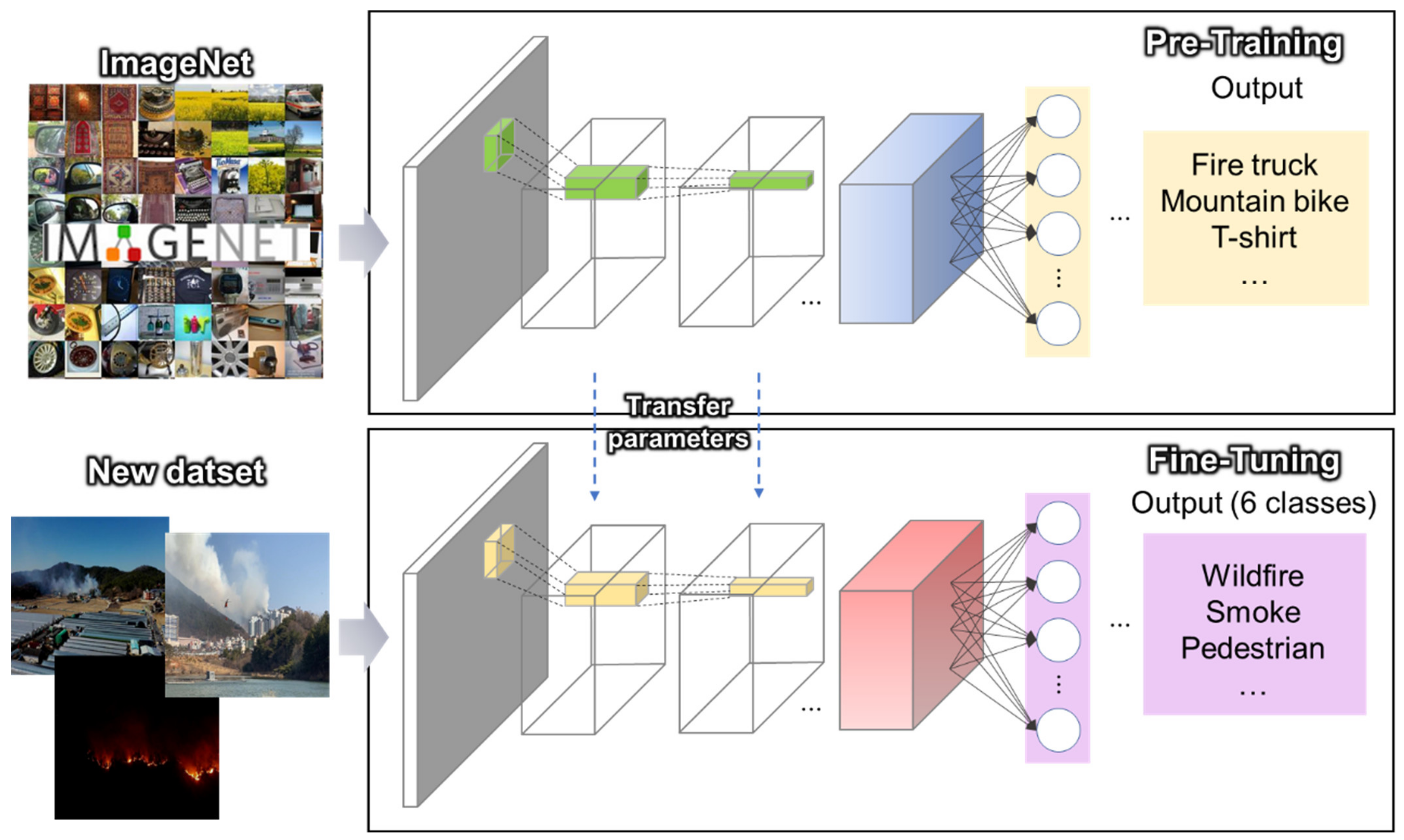
Transfer learning is another approach to prevent overfitting [34]. It is a machine learning method that uses the weights of the pretrained models as weights for the initial or intermediate layers of the new objective model. In computer vision, transfer learning refers mainly to the use of pretrained models. This method is widely used to handle tasks that lack data availability [35]. There are two representative approaches for applying a pretrained model, called a fixed feature extractor and fine-tuning. The fixed feature extractor is a method of learning only the fully connected layer in a pretrained model and fixing the weights of the remaining layers. It is mainly applied when the amount of data is small, but the training data used for pretraining are similar to the training data of the target model. This approach is uncommon for the deep learning of damage detection areas, such as wildfire monitoring images, because of the dissimilarity between ImageNet and the given wildfire images.
On the other hand, fine-tuning not only replaces the fully connected layers of the pretrained model with a new one that outputs the desired number of classes to re-train from the given dataset but also fine-tunes all or part of the parameters in the pretrained convolutional layers and pooling layers by backpropagation. It is used when the amount of data is sufficient, even if the training data are not similar. This is shown in Figure 1.
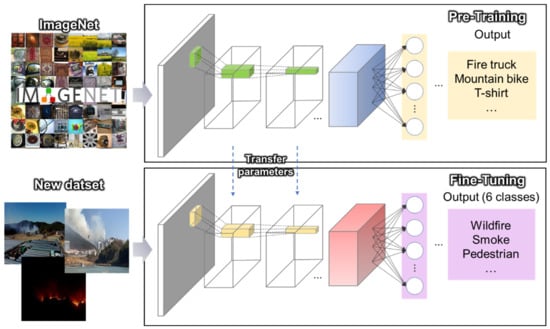
Figure 1.
Transfer learning architecture with fine-tuning using the pretrained CNN model initialized with the weights trained from ImageNet.
The pretrained CNN model from ImageNet [36], which contains 1.4 million images with 1000 classes, is used for transfer learning. However, as there are no labels similar to flame or smoke or other on-site images to assist disaster response in the ImageNet label, fine-tuning is introduced.
3.3. Multilabel Classification Loss
Cross-entropy is defined as the calculation of the difference between the two probability distributions p and q, i.e., error calculations. Cross entropy is used as a loss function in machine learning. However, our framework uses binary cross entropy (BCE), which has commonly been used in the loss function for multilabel classification. The CNN model performs training by adjusting the model parameters such that probabilistic prediction is as similar to ground-truth probabilities as possible through the BCE. In other words, the probability of the output and the target similarly adjusts the model parameters. The BCE loss is defined by the following equation:
where N denotes the total count of images, denotes the probability of class in the target, and denotes the predicted probability of class .
3.4. Proposed Network
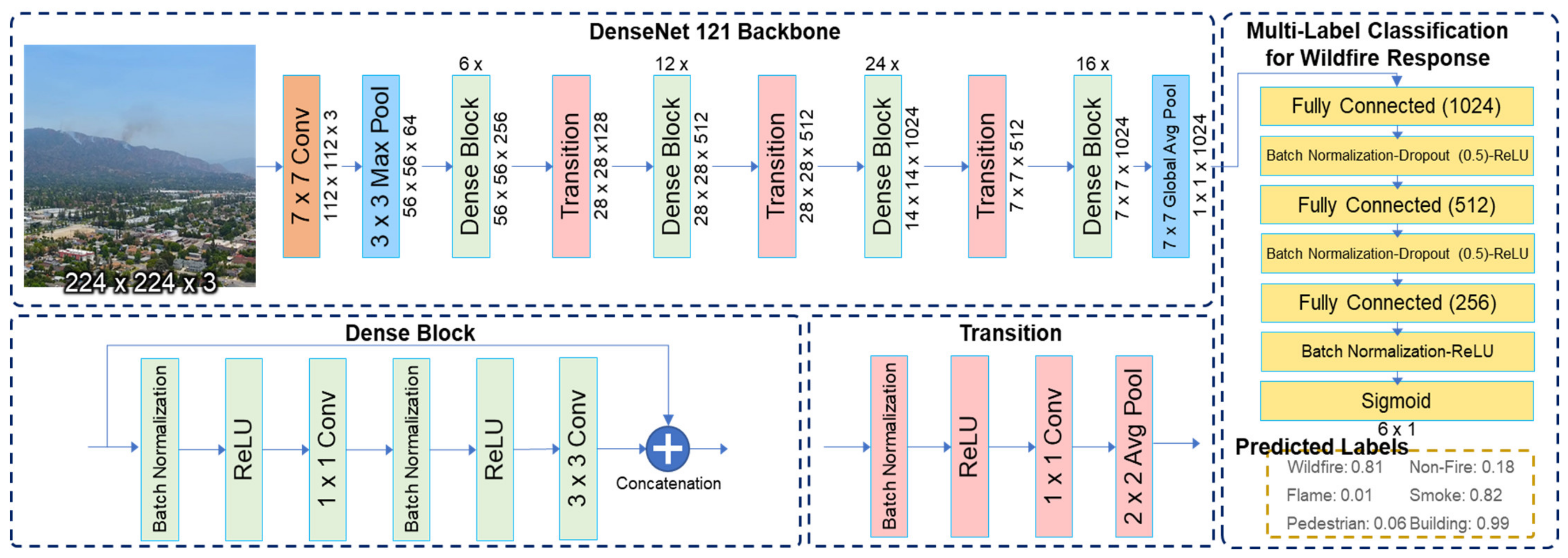
The MLC model used in this study consists of a backbone network pretrained on ImageNet and fully connected layers. In multilabel classification, the training set consists of instances associated with the label set, and the model analyzes the training instances with a known label set to predict the label set of unknown instances. Figure 2 shows an example of a framework for an MLC-based proposed model with DenseNet121 as the backbone. The fully connected layer included dropout [37] and batch normalization [34]. The order of dropout, batch normalization, and rectified linear units (ReLU) were constructed based on the methodology of Ioffe [34] and Li [38].
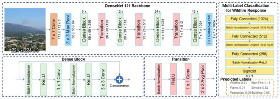
Figure 2.
Proposed approach pipeline: framework of multilabel classification with transfer learning from DenseNet-121 as a backbone network. The probabilities generated by the sigmoid function were independently output at the end of the neural network classifier.
Six classes were printed out, and the model was configured to achieve the following goals required for disaster response during the event of a forest fire: (a) check whether a forest fire has occurred, (b) detect smoke for the early detection of fires, (c) detect the burning area for extinguishing, and (d) detect the areas where human or property damage may occur.
In this study, we selected each of the three pretrained models mentioned above as a backbone network. An MLC model was constructed to provide information that can be supported for wildfire response from CCTV or UAV images. Finally, we compared the performance of each model.
3.5. Performance Metrics
Instances in single-label classification can only be classified correctly or incorrectly, and these results are mutually exclusive. However, the classification schemes in multilabel classification are mutually non-exclusive: in some cases, the predicted results from the classification model may only partially match the elements of the real label assigned to the instance. Thus, methods for evaluating multilabel models require evaluation metrics specific to multilabel learning [39]. Generally, there are two main groups of evaluation metrics in the recent literature: example-based metrics and label-based metrics [40]. Label-based measurements return macro/micro averages across all labels after the performance of the training system, for each label is calculated individually, whereas example-based measurements return mean values throughout the test set based on differences in the actual and predicted label sets for all instances. To evaluate the performance of each model and to verify the effectiveness of transfer learning and data augmentation, this study used macro/micro average precision (PC/PO), macro/micro average recall (RC/RO), and macro/micro average F1-score (F1C/F1O). The abbreviations for evaluation metrics are based on the notations of Zhu [41] and Yan [9]. The metrics are defined as follows:
In the above equations, TP, FP, and FN denote true positives, false positives, and false negatives, respectively, as evaluated by the classifier.
Macro averages are used to evaluate the classification model on the average of all of the labels. In contrast, the micro average is weighted by the number of instances of each label, which makes it a more effective evaluation metric on datasets with class imbalance problems. The F1 score is a harmonic average that considers both precision and recall. Therefore, the F1 score is generally considered a more important metric for comparing the models. In addition, the datasets for MLC generally suffer from data imbalance, and thus, micro-average-based metrics are considered important.
In addition, this study used Hamming loss (HL) and mean average precision (mAP), which are represented by example-based matrices. These metrics are defined as follows:
In the above equations, is the number of samples, is the number of labels, and is the average map of label . Hamming loss is the ratio of a single misclassified label to the total number of labels (considering both the cases when incorrect labels are predicted and when associated labels are not predicted) and is one of the best-known multilabel evaluation methods [42]. The mean average precision was the mean value of the average precision for each class.
3.6. Class Activation Mapping
In the CNN model, the convolutional units of various layers act as object detectors. However, the use of fully connected layers causes a loss in the localizing features of these objects. Class activation mapping (CAM) [43] is used as a CNN model translation method and is a popular tool for researchers to generate attention heatmaps. A feature of CAM is that the network can include the approximate location information of the object even though the network has been trained to solve a classification task [8]. To calculate the CAM value, the fully connected layer is modified with the global average pooling layer (GAP). Subsequently, a fully connected layer connected to each class is attached and fine-tuned. However, it has a limitation in that it must use a GAP layer. When replacing the fully connected layer with GAP, the fine-tuning of the rear part is required again. However, CAM can only be extracted for the last convolutional layer.
Gradient-weighted class activation mapping (Grad-CAM) [44] solves this problem using a gradient. Specifically, it uses the gradient information coming into the last convolutional layer to take into account the importance of each neuron to the target label. In this study, Grad-CAM was used to emphasize the prediction values determined by the classification model and to visualize the location of the prediction target.
4. Results
This section presents the learning process and test results of the MLC model to support wildfire responses. Experiments were conducted in a CentOS (Community Enterprise Operating System) Linux release 8.2.2004 environment with Nvidia Tesla V100 GPU, 32 GB memory, and models were built and trained using PyTorch [45], a deep learning open-source framework.
4.1. Dataset
The dataset used to train and test the deep learning model contained daytime and nighttime wildfire images captured by surveillance cameras or drone cameras downloaded from the Web and cropped images of a controlled fire in the forest captured by a drone by the researchers. This study also included a day–night image matching (DNIM) dataset [46], which was used to reduce the effects of day and night lighting changes, and Korean tourist spot (KTS) [47] datasets generated for deep learning research, which comprise images linked by forest labels containing important wooden cultural properties in the forest. Additionally, wildfire-like images and 154 cloud and 100 sun images were also included as datasets because they have similar properties with early wildfire smoke and flames as the color or shape and are often detected erroneously. As such, they were included in the training dataset to prevent predictable errors in the verification stage and to train the robust model against wildfire-like images.
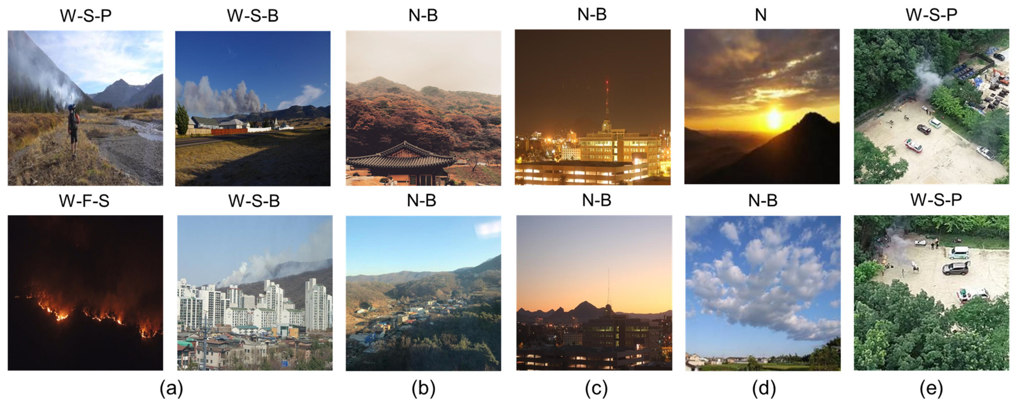
The collected images were resized or cropped to 224 × 224 pixels to consider whether the model is applicable to high-definition images. The datasets included 3,800 images. Figure 3 shows samples of the images.
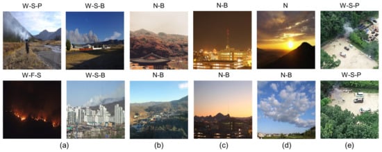
Figure 3.
Resized sample of annotated images for MLC: (a) downloaded from the Web; (b) KTS dataset; (c) DNIM dataset; (d) dataset for error protection purposes; (e) dataset of a controlled fire captured by researchers.
All instances were annotated according to the following classes: “Wildfire”, “Non-Fire”, “Flame”, “Smoke”, “Building”, and “Pedestrian” (each class was abbreviated as “W”, “N”, “F”, “S”, “B”, and “P”, respectively). Table 1 lists the number of images for each designated label set before data augmentation. It consists of 2165 images downloaded from the Web, 1000 images from the KTS dataset, 101 images from the DNIM dataset, 254 images for error protection purposes, and 280 cropped images captured by the researchers. To ensure the annotation quality and accuracy, all of the annotated images were checked twice by different authors.

Table 1.
Number of image datasets for each annotated multilabel instance.
4.2. Data Partition
The dataset used for the experiment was divided into train, validation, and test sets. The test dataset included 2280 images from the entire dataset. The remaining 1520 images were pre-processed by data augmentation techniques, such as rotation, horizontal flip, and brightness, which are typically used in CNN image classification studies to secure sufficient data for learning, as shown in Table 2. Table 1 also lists the number of images for each designated label set after augmentation. Overall, the non-fire label group was the most common, and as the number of multi-labels increased, the number of the label group decreased. In particular, the number of label groups in which pedestrians and houses exist in the wildfire site, which is difficult to obtain, has the lowest number.

Table 2.
Number of images generated by each data augmentation method.
Since drones are generally not perpendicular to the horizon or are inverted when photographing wildfires, the rotation was not set up as extreme, such as at 90° or 180°, but was instead set up between 10° and 350°, considering the lateral tilt of the drone. In addition, if the brightness of the image is too high or too low, the boundary line of the objective target becomes unclear, and the object becomes ambiguous. Therefore, data enhancement was performed between the maximum brightness and the minimum brightness . After data augmentation, the training and test datasets were divided in a ratio of 4:1. In the model learning phase, 912 randomly sampled instances from the training dataset were evenly divided into 10 groups for evaluation using the cross-validation strategy.
The total number of classes of the prepared data was checked, and the distribution is shown in Figure 4. Due to the nature of wildfire response, most of the early detection was performed by smoke, so the number of smoke classes was higher than the number of flame classes. In addition, the wildfire classes and non-fire classes also had an imbalance, and the building and pedestrian classes also had relatively few classes. Since there was an imbalance between the labeling classification table in Table 1 and the overall class distribution in Figure 4, the micro average-based metric evaluation index should be checked.
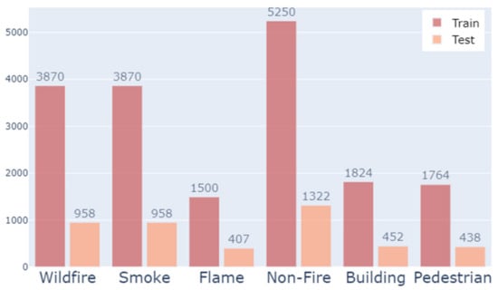
Figure 4.
Histogram of class distribution on multi-label classification datasets after data pre-processing.
4.3. Performance Analysis
This study compared the models with different backbones and verified the efficiency of transfer learning and data augmentation. The model was constructed using training and validation sets that had been partitioned by a 10-fold cross-validation strategy, and the final performance was measured according to each performance metric from the test dataset. The initialized learnable parameters (i.e., hyperparameters) for the CNN-based MLC architectures are listed in Table 3.

Table 3.
Parameters for each CNN architecture.
The models were trained using binary cross-entropy as a loss function with the selected parameters. Each model was trained using a 10-fold cross-validation strategy, and the results were calculated 10 times. The training process using the validation scheme of each model with the selected hyperparameter combination is illustrated in Figure 5. In the case of VGG-16, the training loss fell gently and started at a very high validation loss value, while the training loss of ResNet-50 and DenseNet-121 fell sharply to about epoch 10 at the initial stage and then remained close to zero. However, it was found that DensNet-121 remained lower in terms of the validation learning curve. In the final epoch, epoch 100, it was shown that both the training loss and validation loss recorded the lowest values in DensNet-121.

Figure 5.
Learning curve over epochs (until 100). (a) Training learning curve. Final loss: VGG-16 (0.00789); ResNet-50 (0.00137); DenseNet-121 (0.00048). (b) Validation learning curve. Final loss VGG-16 (0.06790); ResNet-50 (0.03352); DenseNet-121 (0.00318).
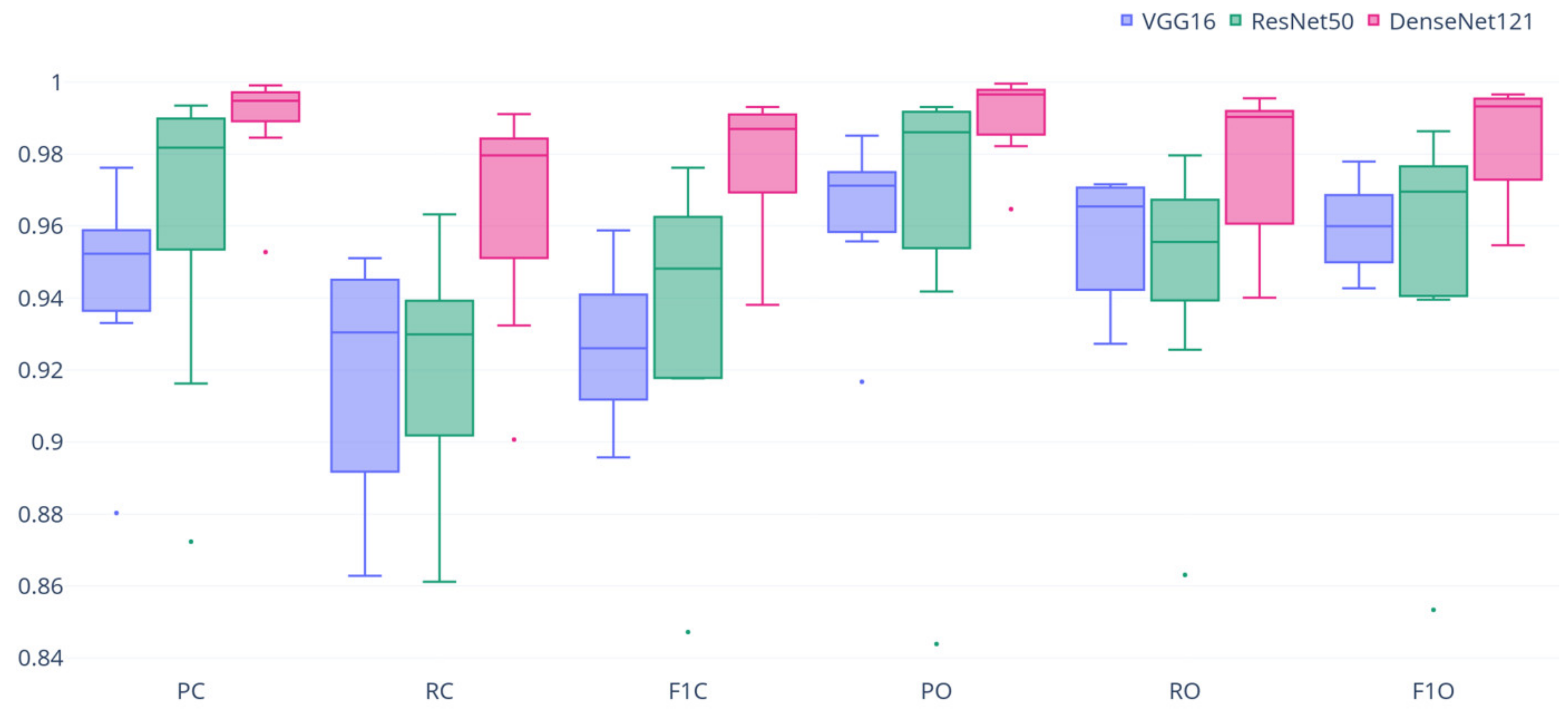
The models were evaluated using the label-based performance metrics, which are shown in Figure 6 as a box plot. All of the proposed models showed good multilabel classification ability using images of forest and wildfire sites for disaster response, with high scores (above 0.9) for most of the evaluation metrics. Among the proposed models, DenseNet-121 not only showed a significantly higher score for all of the evaluation metrics (distribution of the highest box and median value) but the interquartile ranges of each metric result were also typically smaller (i.e., with fewer distributed results) than in other models. Thus, the model maintained consistently high performance over several tests. Table 4 presents the results of the evaluation measurements with the mean and standard deviation.
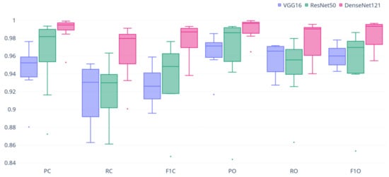
Figure 6.
Boxplot of the 10-fold cross-validation results from performance metrics for MLC model with each backbone network.

Table 4.
Compared performance scores of each backbone network (mean ± standard deviation).
However, an evaluation that only uses label-based measurements cannot highlight the dependencies between classes. Therefore, Table 4 presents example-based scores that consider all of the classes simultaneously and thus are considered more suitable for multilabel problems. The mAP score for the best-performing model (DenseNet-121) was 0.9629, whereas the mAP score for HL was 0.009.
In addition, the per-class score of the area under the receiver operating characteristic curve (ROC-AUC) values of our proposed models were calculated to determine the performance for each class in the image dataset. The ROC curve is a graph showing the performance of the classification model at all possible classification thresholds, unlike the recall and precision values that change as the threshold is adjusted. AUC is a numerical value calculated from the area under the ROC curve and represents the measure of separability. Therefore, the ROC-AUC is a performance metric that is more robust than other performance indicators. AUC values range from 0 to 1, where AUC = 0.5 indicates that the model performed a random guess, and thus, the prediction was the entirely unacceptable. The best performance is when AUC = 1, indicating that all of the instances are properly classified. Table 5 presents the results with mean and standard deviation values.

Table 5.
ROC-AUC scores per class for each model (mean ± standard deviation).
The dataset for the MLC model includes pictures of fires or non-fires (because the results are mutually exclusive). Therefore, the results of two classes—“Wildfire” and “Non-fire”—are calculated in almost the same way. The results of the classes “Wildfire” and “Smoke” were also calculated similarly, as flames are inevitably accompanied by smoke, although this smoke may be invisible because some fires are small or obscured by forests. The accuracy of the pedestrian and building labels was low in all of the models, which can be attributed to the relatively small number of labels assigned to the instances. It was confirmed that the ROC-AUC scores in all of the classes were generally high in the transfer learning algorithm using DenseNet-121 as a network.
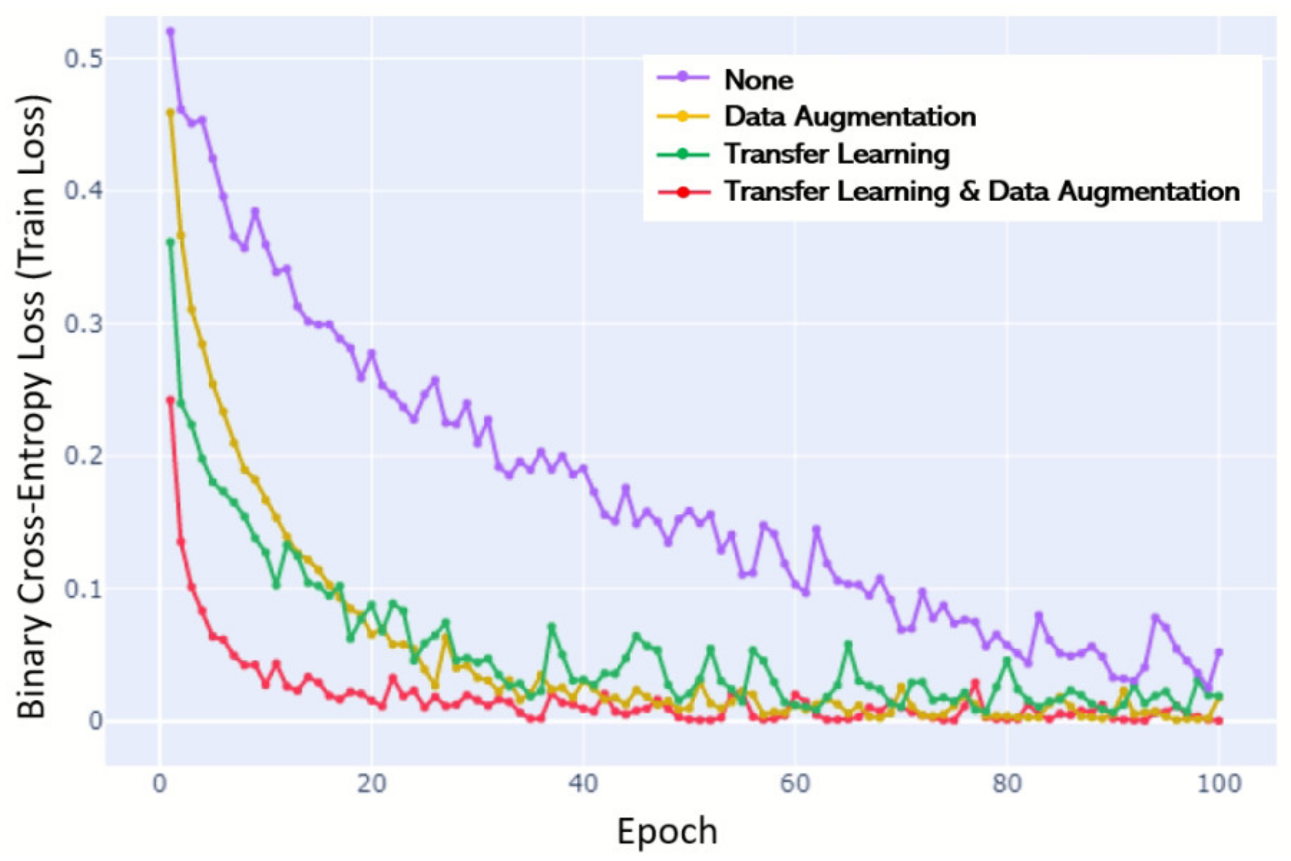
Finally, to confirm the effect of transfer learning and data augmentation on the training model, we removed one data limit overcoming strategies each time using the control variable method and obtained the F1-score and the HL value. This method was implemented for DenseNet-121, which showed the highest performance. The training learning curve over epochs is illustrated in Figure 7. In the training stage, there was a significant difference in the slope of the learning cover curve when no data limit overcoming strategies were used and when one or more strategy was used; a steep learning curve was demonstrated with the strategies; a shallow learning curve was demonstrated without the strategies. When all of the strategies were used, the curve was formed the most rapidly, and the lowest final loss was calculated. This means other models require more practice or attempts before a performance begins to improve until the same level is reached. The curve produced in the case of using all of the strategies was formed the most rapidly, and the lowest final loss score was also calculated. There was no significant difference in the data augmentation and transfer learning effects when looking at the gradient slope or the final loss, but it was shown that the roughness of the curve was further reduced when data augmentation was used. In other words, learning was more stable.

Figure 7.
Learning curve over epochs (until 100) trained by the control variable method. Final loss. Transfer learning and data augmentation (0.00048); data augmentation (0.01807); transfer learning (0.01909); none (0.05216).
Additionally, the test results determined by the evaluation metrics are listed in Table 6. The results of this experiment show that transfer learning can significantly improve multilabel classification performance. With the exception of the transfer learning strategy, the macro average F1-score decreased by 0.0745, the micro average F1-score decreased by 0.0466, and the HL increased by 0.0286. In the case where only augmentation was used, the macro average F1-score decreased by 0.1159, the micro average F1-score decreased by 0.0701, and the HL increased by 0.0412.

Table 6.
F1 scores and Hamming loss values for the models trained by the control variable method.
The performance of transfer learning was further reduced when trained only with the datasets with no data augmentation. Hence, the quantitative number of the datasets required for learning in MLC has a significant impact on the performance of the model.
4.4. Visualization
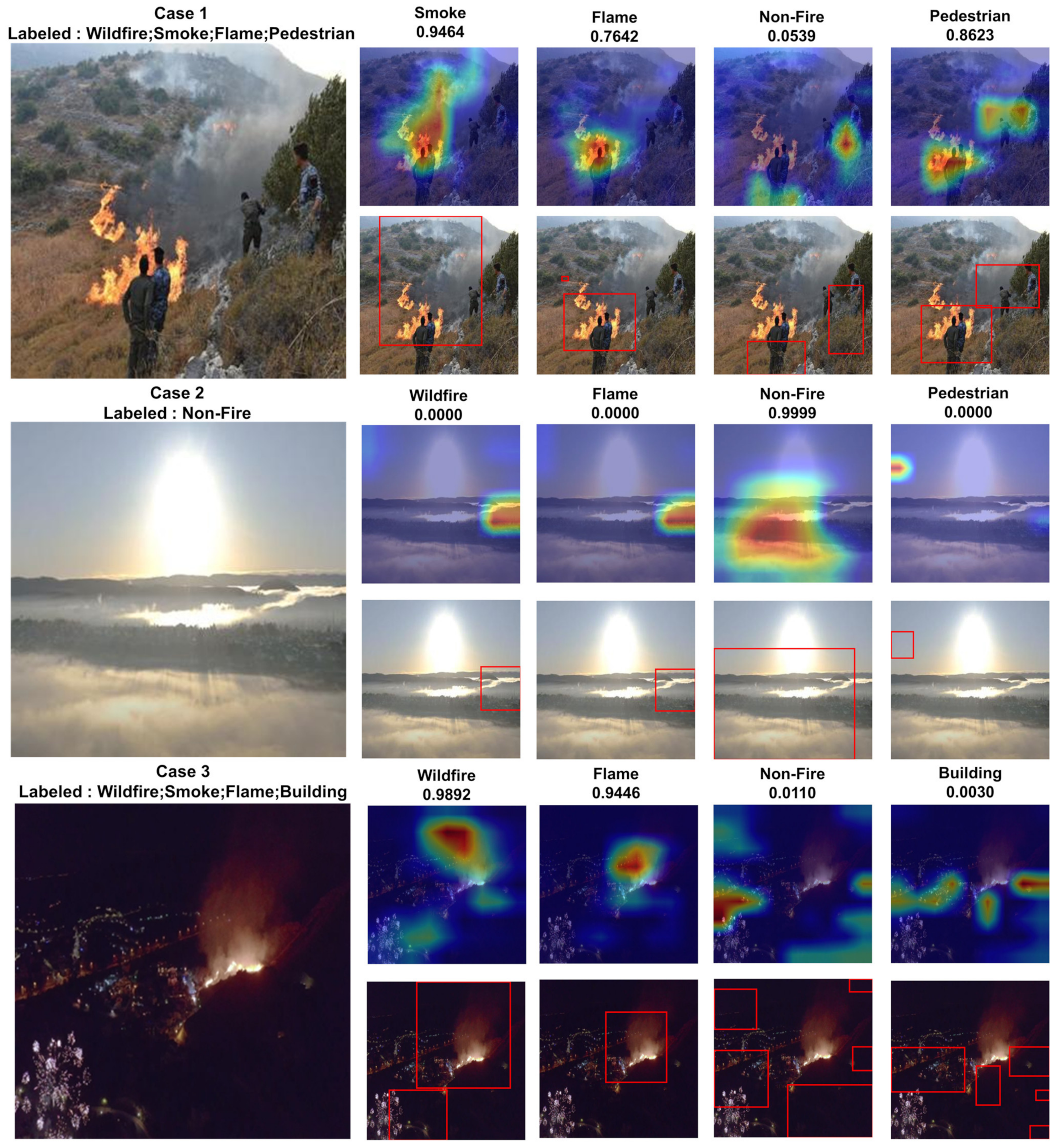
To perform localization, a bounding box is drawn by the thresholding method, which retains over 20% of the grad-CAM result. It also provides a confidence score indicating the extent to which the model’s predictions are true, considering a threshold value of 0.5. Figure 8 and Figure 9 show an example of the results obtained with DenseNet-121 as a backbone.

Figure 8.
Original image (first column) and the heatmap and bounding box (columns 2–5) for a well-classified example (Case 1); an example to review errors for objects with similar colors or shapes (Case 2); and an example of an error for a particular class (Case 3). Case 3 has an error for the building class. The number above each picture is the predictive confidence score.

Figure 9.
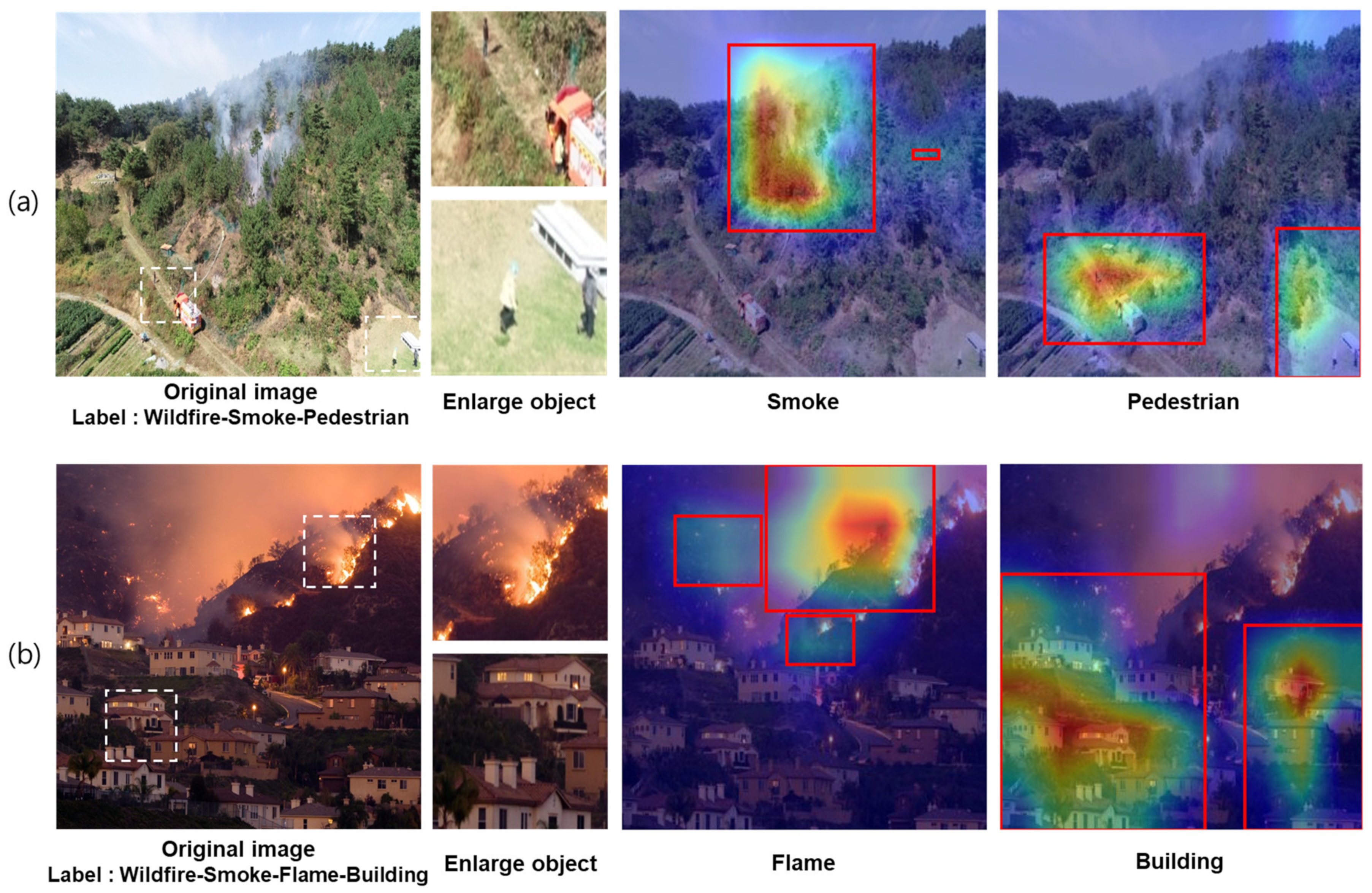
Example of a heatmap and bounding box result for the class that has the possibility of an error. Confidence score (a): Wildfire (0.8117); Smoke (0.8158); Flame (0.0096); Non-Fire (0.1860); Building (0.0006); Pedestrian (0.9952). Confidence score (b): Wildfire (0.8117); Smoke (0.8158); Flame (0.0096); Non-Fire (0.1860); Building (0.0006); Pedestrian (0.9952).
As shown in Figure 8, the sum of the confidence scores between the two classes is almost 100% because the wildfire and non-fire classes are mutually exclusive. Among the test datasets, a Case 1 image was selected as a sample of labeled wildfire with pedestrians, a Case 2 image was selected as a sample with a confusing object, such as sun or fog, that can be treated as a wildfire object for verification. Finally, a sample image with a night fire was selected to evaluate the model in nighttime conditions in Case 3.
In Case 1, the model predicted smoke, flames, non-fire, and a pedestrian with confidence scores of 0.9464, 0.7642, 0.0539, and 0.8623, respectively. The heatmap and bounding box were separated from each other to express the location. Conversely, for non-fire that is not assigned to an instance, a heatmap map without fire or smoke was displayed in the bush area.
Case 2 used an image taken at sunrise in a foggy mountainous area. All of the classes except for the non-fire class showed a score of 0.000, and it was possible to examine whether the model worked correctly to classify the sun and fog, which are frequently used for evaluating errors in wildfire detection.
Case 3 was an image of a wildfire that occurred near a downtown area at nighttime, and fireworks were displayed nearby, which may have some effect on detection. For the wildfire class, a heatmap was formed even in an area unrelated to the wildfire (lower left), which was judged to have detected the smoke generated by the firecrackers on the image. However, although the lighting in the dark at night was considered in the model training process, the heatmap represented the residential area, but the reliability of the building class was still very low (0.0030).
These results were similarly expressed in other test datasets, indicating that the accuracy of the classification was only improved if the CNN model was observable with the naked eye because only clear targets were labeled during the dataset preparation process.
Using an example, Figure 9 shows that the classification model is robust to a small object or noise in a photograph. As shown in Figure 9a, firefighters were dispatched to extinguish the fire in the forest, and nearby hikers were caught on camera. Although the human shape in Figure 9a looks very small, it is detectable with a 0.9952 confidence score, and an approximate location of the object was determined. Figure 9b shows a house with lights on and a nearby forest fire. Despite the similarity of the lamp to the fire image, the heatmap result did not recognize this part as a fire. Thus, the model looked at the appropriate part when identifying each class.
Finally, Figure 10 shows the influence of transfer learning and data augmentation. As discussed in the previous subsection, four cases were classified using the control variable method. For each case, the heatmap and bounding box of a specific class (smoke and person in Figure 10) were visualized, and the probability values were calculated. In the case of not using the data-shortage overcoming strategy, it was found that the heatmap represented the wrong place, and the class that was difficult to distinguish could not be detected at all. (If the value is less than 0.5, it is not treated as a detected value.) Therefore, the accuracy difference is significant if data supplementation strategies are not used for wildfire images, where data are inevitably lacking, as shown in Figure 9 and Figure 10. When a data supplementation method was used, the heatmap distribution was somewhat reasonable, and the confidence value for the class that was to be detected was significantly increased. When both strategies were used, the heatmap distribution was the cleanest, and the positive predictive probability was the highest.
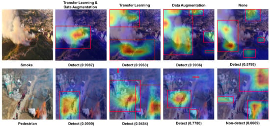
Figure 10.
Sample of the Grad-CAM results depending on the model trained by the control variable method.
4.5. Application
The proposed model was applied to an image captured by the researchers using a DJI Phantom 4 Pro RTK drone, which had an image size of 1280 × 720 high-definition (HD) units. The filming site was composed of a virtual wildfire environment similar to that of a fire created by lighting a drum around the forest.
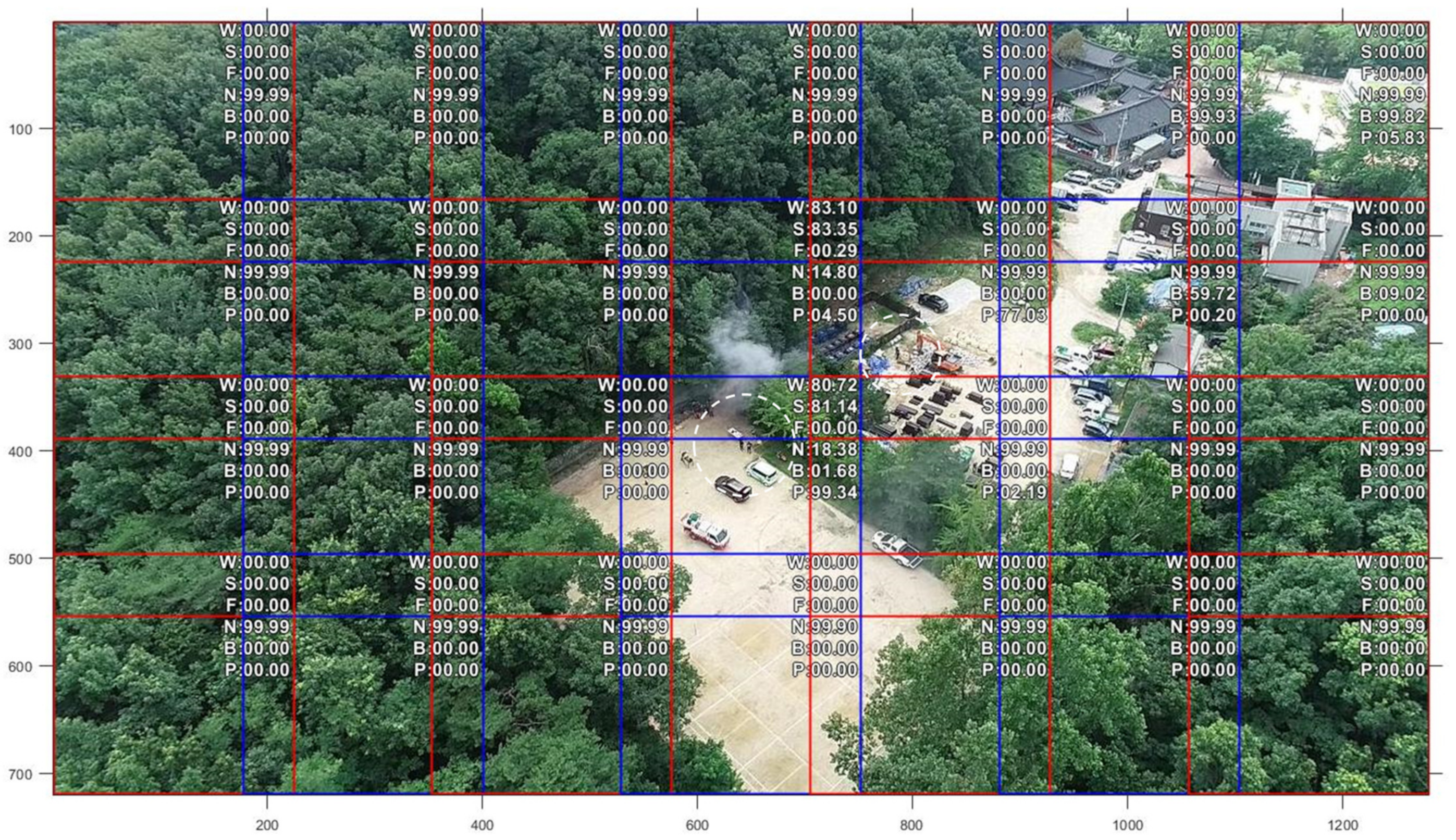
Although the captured HD image can be resized to the input size of the proposed model, downscaling a high-resolution image may result in the loss of information that is useful for classification, and the model may not operate smoothly [48]. Thus, the images were divided into 28 equal parts of 224 × 224, and the model was evaluated for the divided pictures. When the pictures are divided without overlapping parts, there is a possibility of a blind spot where the object to be found is cut off. Thus, the images are divided such that there are overlapping parts. The predicted classification values of each part of the picture were merged into the entire image and were visualized. The results of applying the proposed model to the drone shooting screen are shown in Figure 11. The confidence value was over 50%, and the label corresponding to the photograph part was predicted. In Figure 11, a forest fire was detected based on smoke in the central part of the whole picture. However, there was also an error (9.02%) in the building area, which was important for preserving residential and cultural assets. This error can be explained as follows: the large object was still cut off in the cropped image despite the application of the overlapping method. The white dotted circle was drawn to highlight the area with people, and the model correctly predicted that there were people in the area at 99.34% and 77.03%.

Figure 11.
Sample of model application with the confidence score for each class. The blue and red boxes represent 224 × 224 images.
5. Discussion
In this study, transfer learning and data augmentation were combined to improve the capabilities of the model. Three different pretrained models were used to handle data limitations, data augmentation was performed, and each model was evaluated using label-based evaluative metrics and example-based evaluative metrics. In conclusion, DenseNet-121 surpassed VGG-16 and ResNet-50 in the proposed MLC model. This is confirmed by the results of the evaluation metrics. With the advancement in camera technology, the image resolution increases, but training a CNN to handle large images is particularly difficult. The problems are the cost and learning time caused by excessive computational load in the initial layer. Because of the discrepancy between the image size in these models and the image size taken from the imaging device, we split the high-resolution image into smaller parts and processed them separately. The method proposed in this study loses less data and is expected to better classify small objects compared to scenarios when the original image is reduced in size and only a single image is processed. The proposed framework can be converted into other applications of image-based decision-making systems for disaster response fields to extract redundant information from one object.
Some previous studies used public data for binary classification problems (fire and non-fire). However, a dataset with multiple labels or classes changes according to the requirements of the system, and it is difficult to use the datasets from previous studies. The classified labels were defined to solve the need for a response from the image sources collected at the site. Fire is often accompanied by smoke, which is released faster than flames. The flame of a forest fire is barely visible from a distance. However, the smoke columns caused by fires are usually visible on camera. Therefore, early smoke detection is an effective way to prevent potential fire disasters [49]. Based on the detection of flames, field responders can be informed as to where the flames need to be extinguished. Decision makers for wildfire response, who receive information on the life and property at the fire site, use this basic information to decide on the evacuation route by considering the spot of fire occurrence to preferentially protect the area where there is a possibility of severe damage and to establish a line of defense. Instructions for prioritizing such tasks and for efficiently allocating limited support resources must be provided. Therefore, label categories can be defined for wildfire response and building large image benchmarks for disaster response.
This is a basic study that provides multilabel information of target areas from cameras by applying CNN to wildfire response. Considering that multilabeling was performed manually by the researchers, the distinction between instances was vague in some of the images collected from external data sources. Instances that were too small to distinguish were not labeled to avoid overfitting. In addition, in the case of an instance that cannot be easily distinguished with the naked eye, it was not possible to easily add a class to be classified because of a label classification error.
Therefore, future research should aim to construct a formal annotated data benchmark for wildfire response in deep learning systems to enable the use of field information for supporting disaster decision-makers from the perspective of the wildfire detection algorithm. For example, the state of the wildfire may be understood from the fire shape. Crown fires are the most intense and dangerous wildfires, and surface fires cause relatively little damage. It is also important to identify forest species in disaster areas using videos. If the forests of the target area are coniferous, fires may spread to a large area. To provide this additional information, it is important to ensure communication between photographers, labeling workers, and deep learning model developers. From the perspective of wildfire response, future studies should also aim to develop an integrated wildfire-response decision-support system that can provide decision makers with various insights. Location can be retrieved from the global positioning system (GPS) of drones filming in disaster areas, and this can be combined with data on weather conditions that greatly affect wildfire disasters, such as wind direction, wind speed, and drying rate at the target site. In addition, when combined with a geographic information system (GIS), it is possible to determine the slope of the target area because a steep slope is difficult to control during a wildfire.
6. Conclusions
To the best of our knowledge, previous computer vision-based frameworks for managing fires have only used binary classification. However, in disaster response scenarios, decision makers must prioritize extinguishing operations by considering the range of flames, major surrounding structures such as residential facilities or cultural assets, and residents at the site. Various types of information on the scene of a wildfire can be obtained and analyzed using the photographs from an imaging device. However, annotation work is limited because of a lack of training datasets and the fact that previous wildfire detection research has only focused on binary classification. To solve these problems, we proposed a basic MLC-based framework to support wildfire responses.
The proposed model was verified through well-known evaluation indicators from the dataset selected by the researchers, and DenseNet-121, the most effective of the three representative models, was selected as the final model. Then, we visualized the result through grad-cam, and proposed a method to divide and evaluate each image to prevent data omission when applied to FHD or higher photos according to recently developed camera technology.
Author Contributions
Conceptualization, M.P.; methodology, M.P. and D.Q.T.; data curation, S.L.; writing—original draft preparation, M.P. and S.P.; writing—review and editing, M.P. and S.P.; visualization, M.P. and D.Q.T.; project administration, M.P.; funding acquisition, S.P. All authors have read and agreed to the published version of the manuscript.
Funding
This research was supported by a grant (2019-MOIS31-011) from the Fundamental Technology Development Program for Extreme Disaster Response funded by the Ministry of Interior and Safety (MOIS, Korea).
Data Availability Statement
Data is contained within the article and reference.
Conflicts of Interest
The authors declare no conflict of interest.
References
- Goss, M.; Swain, D.L.; Abatzoglou, J.T.; Sarhadi, A.; Kolden, C.A.; Williams, A.P.; Diffenbaugh, N.S. Climate change is increasing the likelihood of extreme autumn wildfire conditions across California. Environ. Res. Lett. 2020, 15, 094016. [Google Scholar] [CrossRef] [Green Version]
- Guggenheim, D. An Inconvenient Truth; Hollywood Paramount Home Entertainment: Hollywood, CA, USA, 2006. [Google Scholar]
- Roldán-Gómez, J.J.; González-Gironda, E.; Barrientos, A. A survey on robotic technologies for forest firefighting: Applying drone swarms to improve firefighters’ efficiency and safety. Appl. Sci. 2021, 11, 363. [Google Scholar] [CrossRef]
- Chaudhuri, N.; Bose, I. Exploring the role of deep neural networks for post-disaster decision support. Decis. Support Syst. 2020, 130, 113234. [Google Scholar] [CrossRef]
- Muhammad, K.; Ahmad, J.; Baik, S.W. Early fire detection using convolutional neural networks during surveillance for effective disaster management. Neurocomputing 2017, 288, 30–42. [Google Scholar] [CrossRef]
- Akhloufi, M.A.; Castro, N.A.; Couturier, A. UAVs for wildland fires. In Proceedings of the SPIE 10643, Autonomous Systems: Sensors, Vehicles, Security, and the Internet of Everything. International Society for Optics and Photonics, Orlando, FL, USA, 15–19 April 2018; Volume 10643. [Google Scholar]
- Wang, Y.; Dang, L.; Ren, J. Forest fire image recognition based on convolutional neural network. J. Algorithms Comput. Technol. 2019, 13. [Google Scholar] [CrossRef] [Green Version]
- Gong, T.; Liu, B.; Chu, Q.; Yu, N. Using multi-label classification to improve object detection. Neurocomputing 2019, 370, 174–185. [Google Scholar] [CrossRef]
- Yan, Z.; Liu, W.; Wen, S.; Yang, Y. Multi-label image classification by feature attention network. IEEE Access 2019, 7, 98005–98013. [Google Scholar] [CrossRef]
- Hanashima, M.; Sato, R.; Usuda, Y. The standardized disaster-information products for disaster management: Concept and formulation. J. Disaster Res. 2017, 12, 1015–1027. [Google Scholar] [CrossRef]
- Kwak, J.; Bhang, K.; Kim, M.-I. Developing a decision making support information checklist based on analyses of two large-scale forest fire cases. Crisis Emerg. Manag. Theory Praxis 2020, 16, 21–30. [Google Scholar] [CrossRef]
- Li, T.; Zhao, E.; Zhang, J.; Hu, C. Detection of wildfire smoke images based on a densely dilated convolutional network. Electronics 2019, 8, 1131. [Google Scholar] [CrossRef] [Green Version]
- Namozov, A.; Cho, Y.I. An efficient deep learning algorithm for fire and smoke detection with limited data. Adv. Electr. Comput. Eng. 2018, 18, 121–129. [Google Scholar] [CrossRef]
- Taylor, M.E.; Stone, P. Transfer learning for reinforcement learning domains: A survey. J. Mach. Learn. Res. 2009, 10, 1633–1685. [Google Scholar]
- Wybo, J.-L. FMIS: A decision support system for forest fire prevention and fighting. IEEE Trans. Eng. Manag. 1998, 45, 127–131. [Google Scholar] [CrossRef]
- Simonyan, K.; Zisserman, A. Very deep convolutional networks for large-scale image recognition. arXiv 2014, arXiv:1409.1556. [Google Scholar]
- He, K.; Zhang, X.; Ren, S.; Sun, J. Deep Residual Learning for Image Recognition. In Proceedings of the 2016 IEEE Conference on Computer Vision and Pattern Recognition (CVPR), Las Vegas, NV, USA, 27–30 June 2016; pp. 770–778. [Google Scholar]
- Huang, G.; Liu, Z.; Van der Maaten, L.; Weinberger, K.Q. Densely Connected Convolutional Networks. In Proceedings of the IEEE Conference on Pattern Recognition and Computer Vision 2017, Honolulu, HI, USA, 21–26 July 2017; pp. 4700–4708. [Google Scholar]
- Santiago, J.S.S.; Manuela Jr, W.S.; Tan, M.L.L.; Sañez, S.K.; Tong, A.Z.U. Of timelines and timeliness: Lessons from typhoon haiyan in early disaster response. Disasters 2016, 16, 644–667. [Google Scholar] [CrossRef]
- Jung, D.; Tuan, V.T.; Tran, D.Q.; Park, M.; Park, S. Conceptual framework of an intelligent decision support system for smart city disaster management. Appl. Sci. 2020, 10, 666. [Google Scholar] [CrossRef] [Green Version]
- Jain, P.; Coogan, S.C.P.; Subramanian, S.G.; Crowley, M.; Taylor, S.; Flannigan, M.D. A review of machine learning applications in wildfire science and management. Environ. Rev. 2020, 28, 478–505. [Google Scholar] [CrossRef]
- Barmpoutis, P.; Papaioannou, P.; Dimitropoulos, K.; Grammalidis, N. A review on early forest fire detection systems using optical remote sensing. Sensors 2020, 20, 6442. [Google Scholar] [CrossRef]
- Aslan, Y. A Framework for the Use of Wireless Sensor Networks in the Forest Fire Detection and Monitoring. Master’s Thesis, Department of Computer Engineering, The Institute of Engineering and Science Bilkent University, Ankara, Turkey, 2010. [Google Scholar]
- Go, B.-C. IOT technology for forest fire disaster monitoring. Broadcast. Media Mag. 2015, 20, 91–98. [Google Scholar]
- Christensen, B.R. Use of UAV or remotely piloted aircraft and forward-looking infrared in forest, rural and wildland fire management: Evaluation using simple economic analysis. N. Z. J. For. Sci. 2015, 45, 16. [Google Scholar] [CrossRef] [Green Version]
- Chi, R.; Lu, Z.M.; Ji, Q.G. Real-time multi-feature based fire flame detection in video. IET Image Process. 2016, 11, 31–37. [Google Scholar] [CrossRef]
- Park, M.; Tran, D.Q.; Jung, D.; Park, S. Wildfire-detection method using DenseNet and CycleGAN data augmentation-based remote camera imagery. Remote Sens. 2020, 12, 3715. [Google Scholar] [CrossRef]
- Bedo, M.V.N.; De Oliveira, W.D.; Cazzolato, M.T.; Costa, A.F.; Blanco, G.; Rodrigues, J.F.; Traina, A.J.; Traina, C. Fire detection from social media images by means of instance-based learning. In Springer International Conference on Enterprise Information Systems; Springer: Berlin/Heidelberg, Germany, 2015; pp. 23–44. [Google Scholar]
- Sharma, J.; Granmo, O.; Goodwin, M.; Fidje, J.T. Deep Convolutional Neural Networks for Fire Detection in Images. In Proceedings of the International Conference on Engineering Applications of Neural Networks, EANN2017, Athens, Greece, 25–27 August 2017. [Google Scholar]
- Toulouse, T.; Rossi, L.; Campana, A.; Celik, T.; Akhloufi, M.A. Computer vision for wildfire research: An evolving image dataset for processing and analysis. Fire Saf. J. 2017, 92, 188–194. [Google Scholar] [CrossRef] [Green Version]
- Sousa, M.J.; Moutinho, A.; Almeida, M. Wildfire detection using transfer learning on augmented datasets. Expert Syst. Appl. 2020, 142, 112975. [Google Scholar] [CrossRef]
- Muhammad, K.; Ahmad, J.; Mehmood, I.; Rho, S. Convolutional neural networks based fire detection in surveillance videos. IEEE Access 2018, 6, 18174–18183. [Google Scholar] [CrossRef]
- Mikołajczyk, A.; Grochowski, M. Data Augmentation for Improving Deep Learning in Image Classification Problem. In Proceedings of the International Interdisciplinary PhD Workshop (IIPhDW), Swinoujście, Poland, 9–12 May 2018; pp. 117–122. [Google Scholar]
- Ioffe, S.; Szegedy, C. Batch Normalization: Accelerating deep network training by reducing internal covariate shift. arXiv 2015, arXiv:1502.03167. [Google Scholar]
- Mihalkova, L.; Mooney, R.J. Transfer learning from minimal target data by mapping across relational domains. In Proceedings of the 21st International Jont Conference on Artifical Intelligence (IJCAI’09); Morgan Kaufmann Publishers Inc.: San Francisco, CA, USA, 2009; pp. 1163–1168. [Google Scholar]
- Deng, J.; Dong, W.; Socher, R.; Li, L.J.; Li, K.; Fei-Fei, L. Imagenet: A Large-Scale Hierarchical Image Database. In Proceedings of the 2009 IEEE Conference on Computer Vision and Pattern Recognition, Miami, FL, USA, 20–25 June 2009; pp. 248–255. [Google Scholar]
- Srivastava, N.; Hinton, G.E.; Krizhevsky, A.; Sutskever, I.; Salakhutdinov, R. Dropout: A simple way to prevent neural networks from overfitting. J. Mach. Learn. Res. 2014, 15, 1929–1958. [Google Scholar]
- Li, X.; Chen, S.; Hu, X.; Yang, J. Understanding the Disharmony between Dropout and Batch Normalization by Variance Shift. In Proceedings of the IEEE Conference on Computer Vision and Pattern Recognition, Long Beach, CA, USA, 15–20 June 2019; pp. 2682–2690. [Google Scholar]
- Pereira, R.B.; Plastino, A.; Zadrozny, B.; Merschmann, L.H. Correlation analysis of performance measures for multi-label classification. Inf. Process. Manag. 2018, 54, 359–369. [Google Scholar] [CrossRef]
- Zhang, M.L.; Zhou, Z.H. A review on multi-label learning algorithms. IEEE Trans. Knowl. Data Eng. 2014, 26, 1819–1837. [Google Scholar] [CrossRef]
- Zhu, F.; Li, H.; Ouyang, W.; Yu, N.; Wang, X. Learning Spatial Regularization with Image-Level Supervisions for Multi-Label Image Classification. In Proceedings of the IEEE Conference on Computer Vision and Pattern Recognition, Honolulu, HI, USA, 21–26 July 2017; pp. 5513–5522. [Google Scholar]
- Schapire, R.E.; Singer, Y. Boostexter: A boosting-based system for text categorization. Mach. Learn. 2000, 39, 135–168. [Google Scholar] [CrossRef] [Green Version]
- Zhou, B.; Khosla, A.; Lapedriza, A.; Oliva, A.; Torralba, A. Learning Deep Features for Discriminative Localization. In Proceedings of the IEEE Conference on Computer Vision and Pattern Recognition, Las Vegas, NV, USA, 27–30 June 2016; pp. 2921–2929. [Google Scholar]
- Selvaraju, R.R.; Cogswell, M.; Das, A.; Vedantam, R.; Parikh, D.; Batra, D. Grad-Cam: Visual Explanations from Deep Networks via Gradient-Based Localization. In Proceedings of the 2017 IEEE International Conference on Computer Vision (ICCV), Venice, Italy, 22–29 October 2017; pp. 618–626. [Google Scholar]
- Paszke, A.; Gross, S.; Massa, F.; Lerer, A.; Bradbury, J.; Chanan, G.; Killeen, T.; Lin, Z.; Gimelshein, N.; Antiga, L. PyTorch: An imperative Style, High-Performance Deep Learning Library. In Proceedings of the Advances in Neural Information Processing Systems, Vancouver, BC, Canada, 8–14 December 2019; pp. 8024–8035. [Google Scholar]
- Zhou, H.; Sattler, T.; Jacobs, D.W. Evaluating local features for day-night matching. In Springer European Conference on Computer Vision; Springer: Berlin/Heidelberg, Germany, 2016; pp. 724–736. [Google Scholar]
- Jeong, C.; Jang, S.-E.; Na, S.; Kim, J. Korean tourist spot multi-modal dataset for deep learning applications. Data 2019, 4, 139. [Google Scholar] [CrossRef] [Green Version]
- Sabottke, C.F.; Spieler, B.M. The effect of image resolution on deep learning in radiography. Radiol. Artif. Intell. 2020, 2, e190015. [Google Scholar] [CrossRef] [PubMed]
- Zhou, Z.; Shi, Y.; Gao, Z. Wildfire smoke detection based on local extremal region segmentation and surveillance. Fire Saf. J. 2016, 85, 50–58. [Google Scholar] [CrossRef]
Publisher’s Note: MDPI stays neutral with regard to jurisdictional claims in published maps and institutional affiliations. |
© 2021 by the authors. Licensee MDPI, Basel, Switzerland. This article is an open access article distributed under the terms and conditions of the Creative Commons Attribution (CC BY) license (https://creativecommons.org/licenses/by/4.0/).

