Article

Applicability of Data Acquisition Characteristics to the Identification of Local Artefacts in Global Digital Elevation Models: Comparison of the Copernicus and TanDEM-X DEMs

Department of Spatial Sciences, Faculty of Environmental Sciences, Czech University of Life Sciences Prague, Kamýcká 129, 16500 Praha-Suchdol, Czech Republic
*
Author to whom correspondence should be addressed.
Remote Sens. 2021, 13(19), 3931; https://doi.org/10.3390/rs13193931
Submission received: 9 August 2021 / Revised: 26 September 2021 / Accepted: 27 September 2021 / Published: 30 September 2021
(This article belongs to the Special Issue Advances in Global Digital Elevation Model Processing)

Abstract

:
Several global digital elevation models (DEMs) have been developed in the last two decades. The most recent addition to the family of global DEMs is the TanDEM-X DEM. The original version of the TanDEM-X DEM is, however, a nonedited product (i.e., it contains local artefacts such as voids, spikes, and holes). Therefore, subsequent identification of local artefacts and their editing is necessary. In this study, we evaluated the accuracy of the original TanDEM-X DEM and its improved edited version, the Copernicus DEM, in three major European mountain ranges (the Alps, the Carpathians, and the Pyrenees) using a digital surface model derived from airborne laser scanning data as a reference. In addition, to evaluate the applicability of data acquisition characteristics (coverage map, consistency mask, and height error map) and terrain characteristics (slope, aspect, altitude) to the localization of problematic sites, we modeled their associations with the TanDEM-X DEM error. We revealed local occurrences of large errors in the TanDEM-X DEM that were typically found on steep ridges or in canyons, which were largely corrected in the Copernicus DEM. The editing procedure used for the Copernicus DEM construction was evidently successful as the RMSE for the TanDEM-X and Copernicus DEMs at the 90 m resolution improved from 45 m to 12 m, from 16 m to 6 m, and from 24 m to 9 m for the Alps, the Pyrenees, and the Carpathians, respectively. The Copernicus DEM at the 30 m resolution performed similarly well. The boosted regression trees showed that acquisition characteristics provided as auxiliary data are useful for locating problematic sites and explained 28–50% of deviance of the absolute vertical error. The absolute vertical error was strongly related to the height error map. Finally, up to 26% of cells in the Copernicus DEM were filled using DEMs from different time periods and, hence, users performing multitemporal analysis or requiring data from a specific time period in the mountain environment should be wary when using TanDEM-X and its derivations. We suggest that when filling problematic sites using alternative DEMs, more attention should be paid to the period of their collection to minimize the temporal displacement in the final products.

1. Introduction

DEMs are an indispensable data source for various environmental analyses with multiple successful applications, for example, in geology [1], ecology [2], and hydrology [3]. With the growing number of global DEMs available, applications also include multitemporal analyses. Nowadays, global DEMs are increasingly combined for calculations of changes in the glacier mass [4], assessment of topographic changes caused, for example, by volcanic activity [5], or forest change detection [6].
Over the last decades, synthetic aperture radar (SAR) interferometry (InSAR) has become the standard method for obtaining digital elevation models (DEMs) at a global scale [7]. The most recent mission is TanDEM-X that has set out to become a great successor to SRTM [8,9,10,11]. The TanDEM-X mission is a partnership between the German Aerospace Centre (DLR) and Airbus Defence and Space. It is a constellation of two satellites (TerraSAR-X and TanDEM-X), orbiting in a close formation and acquiring high spatial resolution radar images of Earth’s surface [12,13]. DLR is responsible for the operation of the satellites in the orbit, the collection of data during the mission, their interferometric processing, as well as the distribution of the final model to the scientific community. So far, DLR has produced three DEMs at resolutions of 12 m (0.4 arcseconds), 30 m (1 arcsecond), and 90 m (3 arcseconds), respectively. Only the last option (90 m DEM) is, however, available for free, with the other two being available only for scientific use (i.e., via a standard announcement of opportunity process and submission of a scientific proposal). These DEMs are unedited versions resulting from interferometric processing and mosaicking only [14] and they contain artefacts such as voids, spikes, and holes. Remarkably, recent studies evaluating the accuracy of the TanDEM-X DEM highlighted that, despite this drawback, it is superior to other DEMs, and there is no doubt about its unprecedented height accuracy [9,15,16]. Some such comparative studies also visually inspected the global DEMs and emphasized the improvement in detail in the TanDEM-X DEM compared to other global DEMs [17,18].
Global DEMs have been evolving over the long term to meet user requirements for accuracy [19,20,21,22]. For example, the accuracy of the SRTM DEM has been evaluated several times over various surfaces, and such studies laid base for improvements of this model [23,24,25]. The TanDEM-X DEM was first edited by Airbus Defence and Space and made commercially available as WorldDEMTM [26,27]. The vertical accuracy of WorldDEMTM was studied, for example, by Becek et al. (2016) [28] who reported a considerably smaller error compared to SRTM (RMSE of 1.39 m vs. 2.78 m). However, they used almost flat runways as reference data and, therefore, focused mainly on the instrumentation-induced component of the DEM error. More recently, Bayburt et al. (2017) [29] assessed the accuracy in a mountainous terrain and highlighted the higher accuracy of WorldDEMTM compared to other global DEMs. Until recently, WorldDEMTM was the only edited version available, but the need for a freely available edited version fostered further development of editing procedures. González et al. (2021) [30] developed a fully automatic editing algorithm, which is going to be applied at the 30 m resolution, while Huber et al. (2021) [31] developed a semiautomatic framework for generating an edited version of the TanDEM-X DEM at the 12 m resolution. Meanwhile, WorldDEMTM was recently used for the production of three Copernicus DEMs: EEA-10 (0.4 arcseconds), GLO-30 (1.0 arcseconds), and GLO-90 (3.0 arcseconds), with the latter two becoming available for free. Accuracy assessment of the Copernicus DEM was already performed during its production using data derived from the ICESat laser altimetry mission as a reference [32]. However, the same data were also used for calibration of the original TanDEM-X DEM [33]. Consequently, the results of such accuracy assessment might be overly optimistic. In addition, reliability of the ICESat data decreases on steep slopes, and the availability of the ICESat data over mountainous areas is likely limited [34]. Therefore, in this study, we evaluated the absolute vertical accuracy of the Copernicus DEM in European mountains with complex topography using high-resolution LiDAR-derived digital surface models (DSMs).
The editing consists of two general steps. First, problematic sites that require further editing are localized, which is typically performed using various terrain and data acquisition characteristics [26,30,31,35]. Second, the actual editing is performed, which consists of several automatic or semiautomatic processes that include terrain correction (removal of artefacts and voids filling) and hydrological editing (flattening of water bodies and ensuring consistent flow of rivers). Our goals were as follows: (i) to evaluate the success of the editing process (i.e., compare the original version and the edited version of TanDEM-X); (ii) to assess the associations of vertical accuracy of the original version and the edited version of TanDEM-X with terrain (slope, aspect, altitude) and acquisition characteristics (provided by DLR as auxiliary data); and (iii) to evaluate the suitability of acquisition and terrain characteristics for the localization of the TDX90 problematic sites.

2. Materials and Methods

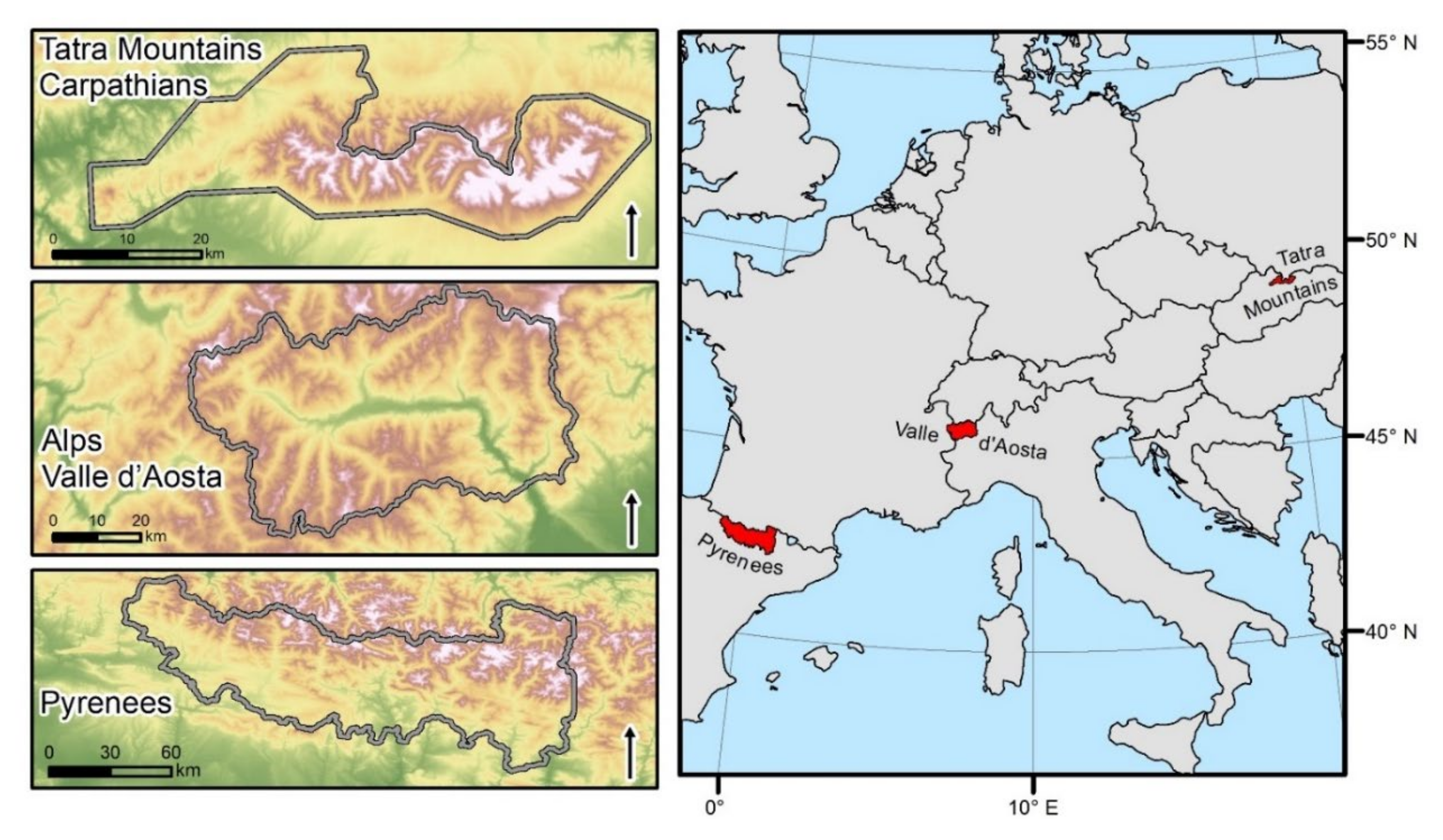
2.1. Study Areas and Airborne LiDAR

Three study areas located in mountain ranges were selected, with the availability of highly accurate airborne laser scanning data for subsequent accuracy assessment being an additional selection criterion. We used a DSM as a reference as it is well-recognized that DEMs derived from SAR height measurement include trees, buildings, and other aboveground structures, thus not representing the bare ground elevation in vegetated and built-up areas [36,37]. However, we used digital terrain models (DTMs) to derive the slope and the aspect of the terrain. The study areas were as follows: the Alps, the Pyrenees, and the Tatra Mountains, which are part of the Carpathians (Figure 1). The study areas cover about 3265 km2 (Alps), 7890 km2 (Pyrenees), and 960 km2 (Tatra Mountains), respectively, with altitudes ranging between 300–4800 m a.m.s.l. (Alps), 450–3400 m a.m.s.l. (Pyrenees), and 500–2700 m a.m.s.l. (Tatra Mountains), respectively. The airborne LiDAR data for Valle d’Aosta in the Italian Alps were collected in 2008 and the DSM derived from those data is freely available for downloading at the 2 m resolution. The airborne LiDAR data for Spain (Pyrenees) were collected between 2008 and 2015 and the resulting DSM is freely available for downloading at the 5 m resolution. The airborne LiDAR data for Slovakia (Tatra Mountains) were collected between 2017 and 2020 and the derived DSM is freely available for downloading at the 1 m resolution [38].

2.2. TanDEM-X, Copernicus, SRTM and NASA DEMs

The TanDEM-X data were collected between 2010 and 2015 [33]. The nominal TanDEM-X acquisitions were taken in the ascending orbits (right-looking observation mode) over the Northern hemisphere. To improve the accuracy in problematic areas such as high mountains, extra acquisitions with different geometries were taken (i.e., adjusting the angle of signal acquisition or using the descending orbits over the Northern hemisphere; [34,39]). The TanDEM-X DEM in the 3-arcseconds resolution (hereinafter referred to as TDX90) was downloaded from https://download.geoservice.dlr.de/TDM90/ (accessed on 9 August 2021). The horizontal and vertical datum of TDX90 is WGS84. Note that the voids present in TDX90 and the auxiliary data were removed and not used in this study. Other components used in this study and provided together with TDX90 as auxiliary data are the coverage map, the consistency mask, and the height error map. The coverage map (COV) indicates a number of valid acquisitions available for mosaicking. The consistency mask (COM) is an auxiliary dataset that indicates height inconsistencies between the individual acquisitions [33]. Two general types of height inconsistencies can be distinguished: (i) small absolute height differences exceeding the corresponding thresholds of height errors, e.g., due to temporal changes (COM2, COM10); and (ii) large absolute height differences arising, e.g., due to phase unwrapping errors or incoherent areas such as shadows or layovers (COM1, COM9). If all the height differences are smaller than a certain threshold, all the input height values are considered consistent (COM8). Note that the category “Smaller inconsistency” (COM2) was present only in a single cell in our study areas and was removed from the analysis. The height error map (HEM) represents the theoretical height error of each TDX90 cell as the standard deviation derived from geometrical considerations and interferometric coherence [8,10,33].
Other DEMs evaluated in this study are the Copernicus DEMs with the resolutions of 3 arcseconds and 1 arcsecond (hereinafter referred to as COP90 and COP30, respectively), which we downloaded from the FTP server cdsdata.copernicus.eu (registration required). The Copernicus DEMs were derived from the TanDEM-X data and were subjected to terrain correction and hydrological editing, including automatic operations as well as manual control. Terrain correction consisted of spikes and holes removal, identification and filling of voids (small voids were interpolated, larger voids—infilled with an alternate DEM), and identification and correction of systematic and random biases [26]. The vertical datum for the Copernicus DEMs is an EGM2008 geoid and the horizontal datum is WGS84 [32].
Besides TDX90 and COP90, which are the main focus of this study, we also used SRTM DEM v3 version (void-filled) with the resolution of 90 m (hereinafter referred to as SRTM90) to provide a direct comparison with this widely used spaceborne DEM. The SRTM data were acquired with a C-band radar sensor attached to Space Shuttle Endeavour during its 11-day-long mission in February 2000 [7]. Each terrain segment was recorded on ascending and descending orbit passes. After its first release in June 2003, SRTM became the most commonly used global DEM. In addition, voids and larger problematic sites in TDX90 were filled using SRTM [26,30,31], and for this reason, it is used as an additional reference in this study. In addition, we also used NASADEM at the 30 m resolution (hereinafter referred to as NASA30), which was recently produced by reprocessing the SRTM data and can be considered as an alternative to COP30 [40]. The vertical datum for both SRTM90 and NASA30 is an EGM96 geoid and the horizontal datum is WGS84. We downloaded the SRTM and NASA30 from the Earth Explorer data portal.
Note that the short-wavelength C-band or X-band radar used for acquisition of the abovementioned DEMs is unable to penetrate the vegetation canopy and reach the bare ground; most of the incoming signals are reflected by various scatterers in the upper part of the canopy [41]. Consequently, the elevation values captured by the sensor are located somewhere between the ground and the top of the vegetation canopy. Hence, the TanDEM-X, SRTM, and NASA DEMs are rather DSMs which represent the surface of the Earth including vegetation, buildings, and infrastructure [42,43,44].

2.3. Accuracy Assessment and Error Modeling

All the datasets were first transformed into the same vertical and horizontal datum. To match the horizontal datum of the spaceborne DEMs and reference LiDAR models, we transformed all the models using the bilinear resampling method into the same UTM zone. LiDAR DSMs were aggregated using the mean value to the same resolution. The vertical datum of all the datasets is represented as orthometric heights except for TDX90, which represents ellipsoidal heights. In order to match the ellipsoidal heights of TDX90 with the orthometric heights of other models, we used an Earth Gravitational Model (EGM2008).
We calculated height differences between the reference LiDAR DSM and the spaceborne DEMs. We used the differences to calculate the mean error (ME) and the root mean square error (RMSE) expressed as follows:
ME = 1 n i = 1 n h DEMi h REFi = 1 n i = 1 n Δ h i
R M S E = 1 n i = 1 n Δ h i 2
where n is the total number of sampled cells, hDEMi is the ith height from the global DEM, and hREFi is the corresponding height from the LiDAR DSM. The RMSE measures the mean square magnitude of errors. This measurement gives more weight to large deviations such as outliers. Therefore, in addition, we also calculated robust metrics (less affected by outliers [45,46]); namely, we calculated the absolute deviation at the 90% quantile (LE90) and the mean absolute error expressed as follows:
L E 90 = Q Δ h 0.9
MAE = 1 n i = 1 n h DEMi h REFi = 1 n i = 1 n | Δ h i |
where n is the total number of sampled cells, hDEMi is the ith height from the global DEM, and hREFi is the corresponding height from the LiDAR DSM. LE90 was calculated as the 90th percentile of the manually sorted absolute height differences (i.e., 90% of the differences are less than or equal to this value).
In addition, we aimed at evaluating the suitability of acquisition and terrain characteristics for the localization of the TDX90 vertical error. We combined the auxiliary data (HEM, COM, and COV) and the terrain characteristics (slope, aspect, and altitude) to model the absolute vertical error (the difference between TDX90 and LiDAR DSM). The terrain slope and aspect were derived from a LiDAR digital terrain model at the 90 m resolution (i.e., we first aggregated the digital terrain model to the 90 m resolution using the mean values and then calculated the terrain characteristics) [47,48]. We used Horn’s algorithm with a 3 × 3 cell neighborhood implemented in ArcGIS (version 10.8.1).
We evaluated the relationships between the differences (absolute values) and the explanatory variables using boosted regression trees (BRT). We used functions provided by Elith et al. (2008) [49] and R package gbm version 2.1.5. [50]. The models were fitted with the maximum number of trees of 5000, the learning rate of 0.05 (controls the rate at which the model complexity is increased; small values allow the model to grow more trees), the bag fraction of 0.5 (the proportion of the data used when selecting the optimal tree number), and without interaction terms (i.e., the tree complexity of 1). The absolute vertical error was modeled specifying the Gaussian error distribution. To estimate the optimal number of trees, we used a fivefold cross-validation. This consisted of randomly dividing the dataset into five independent partitions, calibrating the model on the basis of four partitions and, subsequently, validating it with the remaining one. This procedure was repeated five times, each time leaving out another partition. At each iteration, the residual deviance was calculated and the number of trees giving the best model (i.e., the lowest residual deviance) was identified [49]. The overall performance was assessed using the total deviance explained (i.e., the proportion of the variance explained by the model), which was calculated by dividing the difference between the mean total deviance and the estimated fivefold cross-validated residual deviance by the mean total deviance. In order to estimate the utility of the variables for the absolute vertical error modeling, we calculated the relative importance of each variable (i.e., the contribution of each variable to the model fit [49]). The importance of each variable was scaled so that the sum adds to 100 and represents how much the model was improved by including that particular variable. The models were fitted in R, version 3.6.0 (R Development Core Team).

3. Results

3.1. Absolute Vertical Accuracy of TDX90, COP90, COP30, SRTM90, and NASA30

First, we performed an overall accuracy assessment of all the DEMs (TDX90, COP90, SRTM90, COP30, and NASA30). The mean differences between the reference DSM and the spaceborne DEMs were small—up to ± 2 m, except for TDX90 in the Alps (Table 1). In terms of LE90, the absolute vertical accuracy of TDX90 was the highest in the Pyrenees, followed by the Tatra mountains and the Alps. The differences between the RMSE and the MAE are the most striking features of this comparison (Table 1). While according to the RMSE, SRTM is a better model than TDX90 in all areas, the situation is reversed when using the MAE (which is less affected by outliers). Note also that the difference between the RMSE and the MAE is considerably higher for TDX90 than for SRTM90. This indicates that TDX90 contains many cells with a relatively large error (i.e., artefacts such as spikes and holes). Importantly, the absolute vertical accuracy of COP90 is better than that of TDX90 in all the study areas (and it also outperforms SRTM90), which shows that the editing process was successful. When comparing DEMs with the 30 m resolution, COP30 mostly outperformed NASA30.

3.2. Association of the Accuracy of TDX90, COP90, SRTM90, COP30, and NASA30 with Terrain Characteristics

Our results show a noticeable effect of the terrain slope on the vertical accuracy of all the evaluated DEMs (Table 2), with the increasing slope leading to decreasing accuracy. All the models tended to slightly underestimate or overestimate the reference DSM throughout all the slope categories, with the notable exception of the steepest slopes (>40°) where TDX90 considerably underestimates the reference DSM. In terms of LE90, TDX90 had a higher accuracy than SRTM for all the slope categories, except for the steepest slopes (>40°). When using the MAE, on the other hand, the accuracy of TDX90 and SRTM was more or less the same in the steepest category (>40°). The high difference between LE90 and the MAE implies a high presence of outliers in TDX90 in this category (i.e., slopes >40°). COP90 had a similar or better accuracy than TDX90 in all the evaluated categories of slopes regardless of the validation metric and performed better than SRTM90. As for the models at the 30 m resolution, COP30 was more accurate than NASA30 throughout all the slope categories.
The terrain aspect also affects the global DEMs’ vertical accuracy. The highest variation of the accuracy with respect to the terrain aspect was observed in the Alps, where LE90 of TDX90 varied from 47.48 m (in the areas with the 90–112.5° aspect) to 7.92 m (in the areas with the 337.5–360° aspect). In the Alps, LE90 of TDX90 was higher in the areas with east- and west-facing slopes and lower in the areas with north- and south-facing slopes (Figure 2). LE90 varied with the aspect by up to 9.42 m and 4.41 m for COP90 and SRTM90 and by up to 12.18 m and 4.76 m for COP30 and NASA30, respectively. The strong dependence of accuracy on the aspect in the Alps is a coincidence of several factors rather than a generally presented pattern in TDX90. Indeed, in the remaining areas (the Pyrenees, the Tatra Mountains), the effect of the aspect on the vertical accuracy was much smaller compared to the Alps (Figure 2). The first factor contributing to this phenomenon is that the study area of the Alps has steeper slopes than the other areas. The other factor is the generally lower number of acquisitions compared to the other areas. For example, the maximum number of acquisitions in the Alps was eight, compared to as much as thirteen in the Pyrenees. This resulted in large outliers concentrated in a few places with mainly east and west orientation and, hence, in the inflation of LE90 (see Figure 3 for the map of the slope, the aspect, and the absolute vertical error of TDX90 in the Alps’ study area).

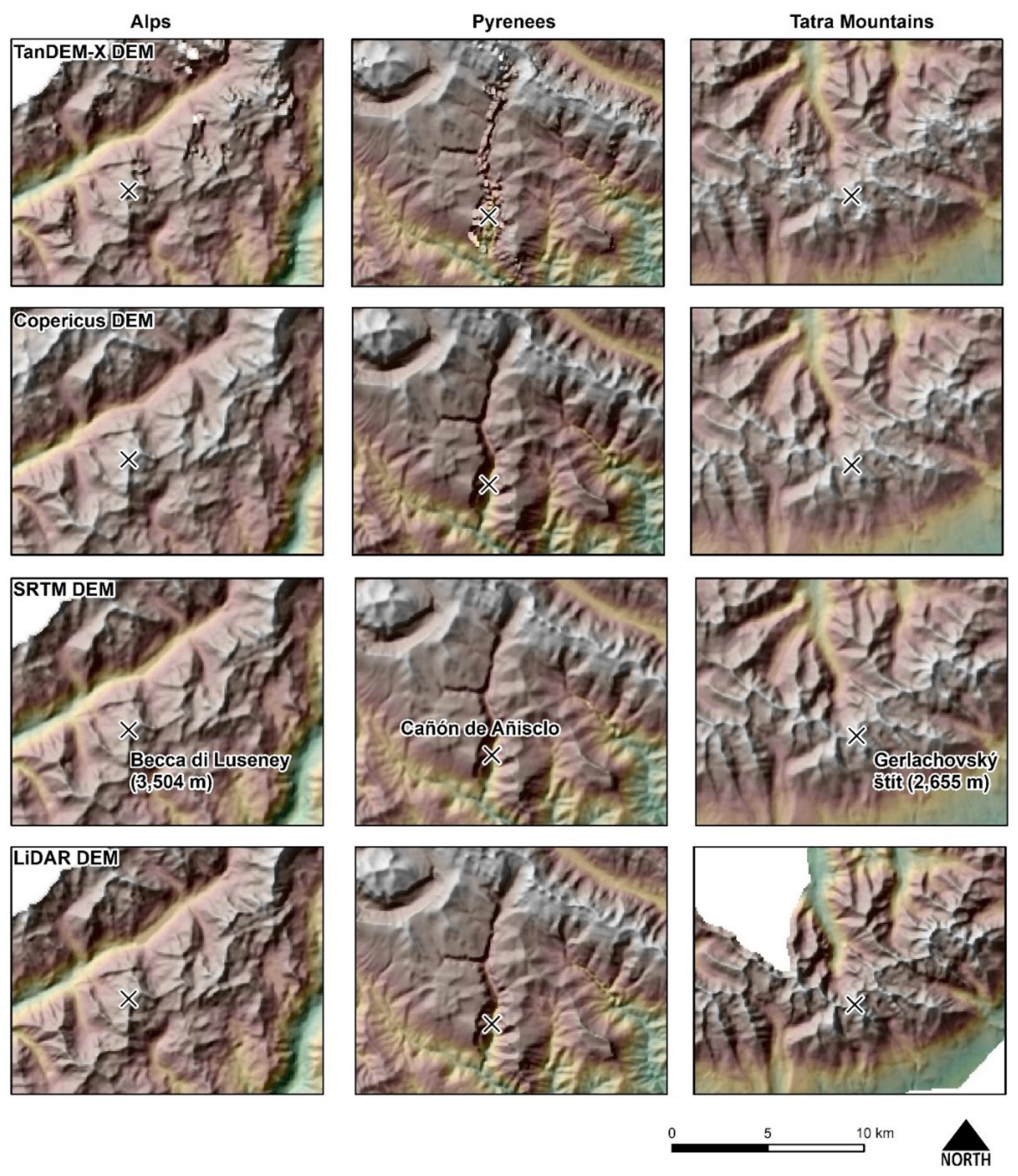
3.3. Visual Inspection of the Most Problematic Sites

In addition to the above analyses, we also assessed the improvement in COP90 compared to TDX90 visually (Podobnikar, 2009). TDX90 represents the topography well in most places but it fails in some parts (see examples of such problematic parts in Figure 4). Note that in these sites, COP90 and SRTM90 correspond with the LiDAR DSM much better than TDX90. In general, the largest errors are observed on steep slopes, sharp ridges, and in deep valleys, which is expected as the mountain environment is challenging for SAR acquisitions (Toutin, 2002). In the Alps (Valle d’Aosta), artefacts are rather scattered on individual ridges (for example, near the Becca di Luseney mountain). In the Pyrenees, few ridges show similar errors as in the Alps; the most obvious problem is, however, the absence of the Cañón de Añisclo. The highest concentration of artefacts can be found in the highest part of the Tatra mountains (around its highest peak Gerlachovský štít) where multiple peaks and ridges are poorly represented in TDX90 (Figure 4).

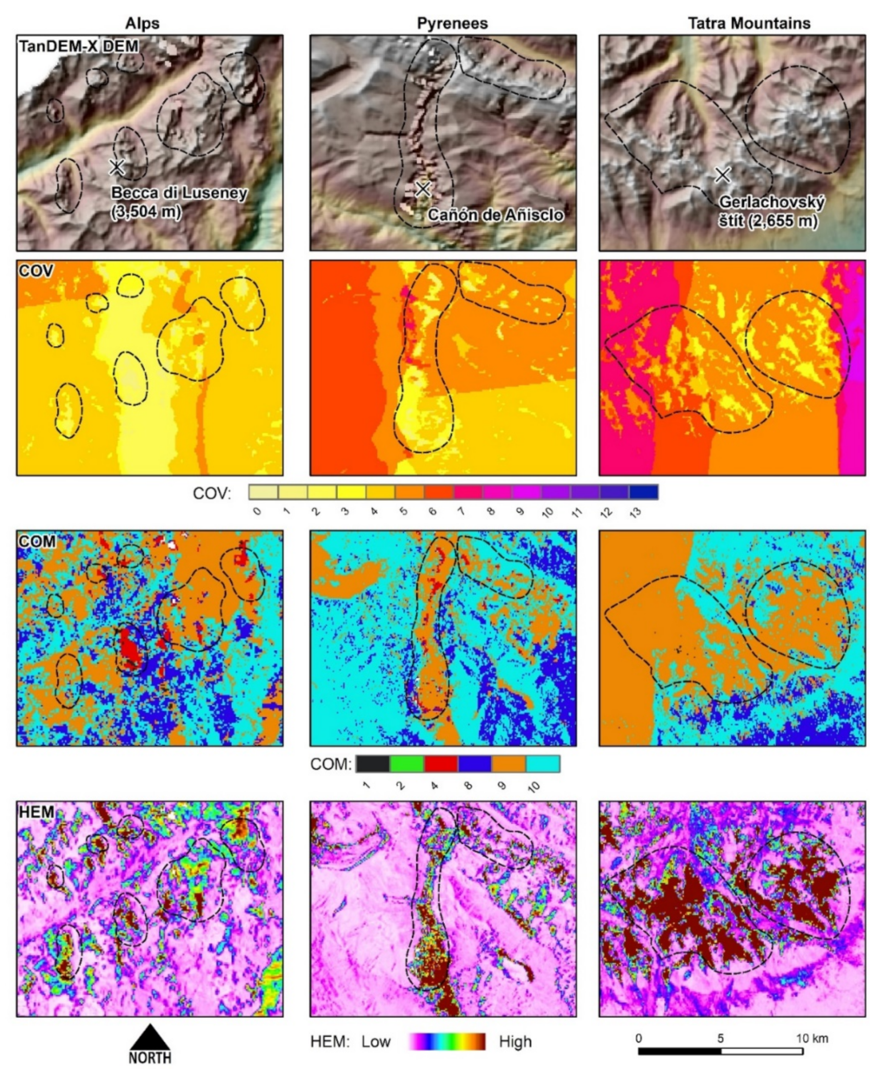
3.4. Association of the Accuracy of TDX90 with Auxiliary Characteristics (COM, COV)

First, we assessed the vertical accuracy of TDX90 with respect to the height inconsistencies among the contributing scenes. We also included COP90 and SRTM90 to provide a comparison, but we did not include COP30 and NASA30 in this part of evaluation to avoid influence of the horizontal resolution on the vertical error. TDX90 showed great accuracy for pixels in the COM8 category (all heights were consistent), in which LE90 was between 3.6 m and 5.7 m. COP90 and TDX90 showed similar accuracies in terms of LE90, but in terms of the RMSE, COP90 showed better accuracy than TDX90, indicating that some minimum editing in this category was successfully performed (Table 3). However, only less than 20% of cells in our study areas fall into this category. Most of the cells in our study areas fall into the categories COM9 and COM10 (categories indicating larger or smaller inconsistency, respectively, with at least one consistent height pair). These categories are associated with lower accuracy of TDX90 than the “All heights are consistent” category (COM8). LE90 of the cells in the category COM9 for TDX90 and COP90 ranged between 10.3 m and 41.9 m and between 9.2 m and 17.8 m, respectively, and LE90 of the cells in the category COM10 ranged between 6.6 m and 9.8 m and between 7.0 m and 9.7 m, respectively. It is, therefore, evident that editing of the cells was required—particularly in the COM9 category—and that it was successful as LE90 is considerably lower for COP90 than for TDX90 (Table 3).
A very small proportion of cells (less than 1% in all the study areas) fell into the categories “Only one coverage” (COM4) or “Larger inconsistency” (COM1). Most cells falling into these categories were found in the study area of the Alps and, despite their relatively low proportion, they can still encompass tens of square kilometers. LE90 of these categories for TDX90 and COP90 ranged between 225.4 m and 558.6 m and between 53.5 m and 78.9 m, respectively. Thus, again, the improvement in accuracy and successful editing of COP90 is evident. Despite this improvement, however, the accuracy of COP90 in the categories COM1 and COM4 was considerably lower than in the categories COM8, COM9, and COM10, respectively (Table 3). This is likely due to the fact that for filling in the problematic sites in TDX90, SRTM was predominantly used, and the accuracy of SRTM90 in such cells is also low. The poor accuracy of both these models in such cells indicates that they represent locations that are likely problematic for synthetic aperture radar (SAR) interferometry in general.
The number of acquisitions ranged between 2 and 8 in the Alps, between 2 and 13 in the Pyrenees, and between 3 and 10 in the Tatra Mountains, respectively. Therefore, we assessed the role of the number of acquisitions within the consistency mask categories COM8, COM9, and COM10 (the results for COM1 and COM4 are not shown as they have poor accuracy anyway, see above). Our results show that with an increasing number of acquisitions, accuracy within individual consistency mask categories (COM8, COM9, and COM10) generally increases. Cells falling within the “All heights are consistent” category (COM8) with at least three valid acquisitions (COV3) provide excellent accuracy; in these categories, LE90 of TDX90 ranged among the COV categories between 3.8 m and 6.5 m in the Alps, between 3.9 m and 6.5 m in the Pyrenees, and between 2.5 m and 5.1 m in the Tatra Mountains, respectively (Table 4). Cells in the category “Smaller inconsistency but at least one consistent height pair” (COM10) with a minimum of three valid acquisitions (COV3) also show a relatively good accuracy; depending on the study area, LE90 was slightly higher or lower than 10 m (Table 4). The most problematic cells of this subgroup in terms of accuracy are those with larger inconsistencies but at least one consistent height pair (category COM9). In particular, the combination of large inconsistencies (COM9) and a relatively low number of acquisitions (COV < 6) results in poor accuracy. Importantly, we observed a considerable improvement in COP90 over TDX90 in almost all the COM/COV categories (Table 4).

3.5. Utility of Auxiliary Data and Terrain Characteristics for the Identification of Problematic Sites

Here, we aimed at evaluating the suitability of the acquisition and terrain characteristics for estimating the absolute vertical error (TDX90 minus the LiDAR DSM). Visual assessment of the data acquisition characteristics showed that the problematic sites tended to be located in the pixels with a relatively low number of acquisitions (COV) in combination with height inconsistencies among individual acquisitions (COM) and with high values of the theoretical height error (HEM; Figure 5). The BRT models of the absolute vertical error (|dh|) explained between 28% and 50% of the deviance. The auxiliary characteristics height error map (HEM) and consistency among the scenes (COM) together explained most of the explained variability (between 77% and 93%). The DLR-provided estimate of the magnitude of errors, the HEM, proved to be highly suitable for the identification of the problematic sites as this parameter in itself explained more than 60% of the explained variability (Table 5). The effect of COM differed between the study areas, showing a large effect in the Pyrenees, a moderate effect in the Alps, and no effect in the Tatra Mountains. The effect of the remaining variables was minimal (see Table 5).
Wessel et al. (2018) [8] suggested that the HEM can be regarded as a reliable estimate of the vertical error, but, more recently, Gdulová et al. (2020) [10] showed that the HEM underestimates the vertical error. To further analyze the relationship between the HEM and the vertical error, we generated partial dependency plots of this variable (Figure 6). The cells with HEM values lower than approximately 0.5 m showed excellent accuracy, but above that value, the difference between TDX90 and the LiDAR DSMs started to increase considerably. The plots showed a gradual increase of the absolute value of the height error up to the HEM value of 2–3 m, with minimal changes or even a slight decrease as the HEM continued to increase (note that the decrease cannot be properly evaluated due to relatively few measurements of relatively high HEM values). The modeled relationship between the absolute vertical error and the HEM corresponds with the measured error (see boxplots in Figure 6).

4. Discussion

In this study, we assessed the vertical accuracy of five global DEMs derived from TanDEM-X and/or SRTM in three major European mountain ranges. COP90 shows considerable improvement over TDX90 and SRTM90. Overall LE90s of TDX90 and COP90 were 17.98 m and 12.69 m, 6.81 m and 6.77 m, and 11.98 m and 11.51 m in the Alps, in the Pyrenees, and in the Tatras (Carpathians), respectively, when compared to the LiDAR DSMs. COP30 showed a similar accuracy to its coarser resolution counterpart COP90 and performed better than NASA30.
The accuracies reported in our study areas are generally lower than those reported in other studies but they reflect the challenging mountain environment [8,9,15]. Despite the postprocessing efforts by the German Aerospace Center that included inspection of the differences between the TanDEM-X DEM and the SRTM–C-band DEM [33], our evaluation and visual inspection revealed that in the mountain environment, TDX90 contains many cells with a relatively large error (i.e., artefacts such as spikes and holes), which is not a surprise as TDX90 is a nonedited product derived from interferometric radar processing and mosaicking only. On the other hand, it should be highlighted that the area needing improvement is relatively small. For example, less than 7% of all the cells in the Pyrenees study area were edited or filled with external DEMs (see Table 6), which is remarkable as the mountain environment is challenging for SAR acquisitions and complies with prior studies that highlighted the excellent accuracy of the TanDEM-X DEM [8,9,10]. In general, the largest errors are observed on steep slopes, sharp ridges, and in deep valleys.
The Copernicus DEMs, on the other hand, are edited; spikes and holes were identified and voided out, small voids were filled by interpolation, larger voids were infilled using alternative DEMs [32]. Indeed, both performed better than TDX90, SRTM90, and NASA30 in all the study areas, which indicates that the editing process was successful. This corresponds with prior reports. Guth and Geoffroy (2021) [51] reported that the accuracy of COP90 was superior to other global DEMs over eight study sites located in the USA and Europe. Besides, the Copernicus DEM documentation reports that the absolute vertical accuracy in terms of LE90 is below 2 m and approximately 50% of Europe and more than 60% of the rest of the world, respectively, has an accuracy better than 2 m [32].
The gaps and problematic sites in COP90 were, however, filled with external reference data. The extent of this infilling with external data can reach up to tens of percent in mountainous areas, such as our study areas. This information is stored in the filling mask (FLM; part of the Copernicus DEM’s auxiliary information), which indicates the source of filled pixels (i.e., the respective global DEM used for filling in the particular area). The prevailing models used for filling of the Copernicus DEMs in our study areas were the SRTM and ASTER DEMs, which were, however, acquired at different time periods from the TanDEM-X data (see Figure 3 and Table 6 for a summary of the number of cells that were replaced by data from other models). Consequently, it is necessary to bear this fact in mind as it also means that the suitability of the Copernicus DEMs for multitemporal analysis in the mountainous environment is limited and users should always consult auxiliary data such as the filling mask before any analysis requiring data from a specific time period [30,32] and remove such areas from analysis. Besides, when using TDX90, for example in combination with the upcoming TanDEM-X Change DEM [52], users should use auxiliary data, such as the HEM, COM, and COV, to identify possible problematic areas [10].
It is fair to note here that temporal misalignment between datasets used in this study might have also affected our results. Due to the limited data availability, it is a common practice to evaluate accuracy of global DEMs using the reference data from different timepoints [9,53,54]. Our study is not an exception, and the time of acquisition should be considered when interpreting the results. The LiDAR data of the Alps were collected in 2008 (i.e., before the TanDEM-X mission), the acquisition time over the Pyrenees more or less overlapped with the TanDEM-X mission, and the data for the Tatra Mountains were acquired a few years after the mission. Obviously, all the reference data were acquired several years after the SRTM mission (February 2000; [7]). Consequently, additional bias between the SRTM, TanDEM-X, and reference DSMs that might have resulted from vegetation growth or deforestation is to be expected.
Our results indicate that data acquisition characteristics that are available as the TDX90 auxiliary data (HEM, COM, COV) can be used for the identification of problematic sites with large errors. These results are consistent with prior studies that evaluated the role of acquisition characteristics on the TDX90 accuracy [8,10,29,55]. We identified the cells falling within the categories “Only one coverage” (COM4) and “Larger inconsistency” (COM1) as highly problematic, with a high risk of erroneous measurement and presence of artefacts. The cells in these categories should be subject to a thorough accuracy evaluation before being included in any analysis (less than 1% of cells in our study areas). Our results show that with the increasing number of acquisitions, the accuracy generally increases as the error can be averaged and smaller deviations are obtained in the resulting height estimate [34]. The cells within the “All heights are consistent” category (COM8) provide excellent accuracy. The cells within the “Smaller inconsistency but at least one consistent height pair” category (COM10) also show a relatively good accuracy, depending on the study area. The combination of large inconsistencies (COM9) and a relatively low number of acquisitions (COV < 6) results in poor accuracy. The DLR-provided estimate of the magnitude of errors, the HEM, proved to be highly suitable for the identification of the problematic sites. A quick inspection of a differential DEM or hill-shaded terrain only in the areas of the highest HEM values can facilitate quick (albeit rough) identification of problematic sites.

5. Conclusions

We have shown that the Copernicus DEM at the 30 m and 90 m resolution is clearly a more accurate representation of Earth’s surface than the TanDEM-X, SRTM, and NASA DEMs. The RMSE for the TanDEM-X DEM and the Copernicus DEM improved from 45 m to 12 m, from 16 m to 6 m, and from 24 m to 9 m for the Alps, the Pyrenees, and the Carpathians, respectively. In other words, editing used for the generation of the Copernicus DEM from the TanDEM-X DEM was successful. However, the Copernicus DEM includes data from different time periods and, hence, their value for multitemporal analyses is limited. We suggest that when filling problematic sites using alternative DEMs, more attention should be paid to the period of their collection to minimize the temporal displacement in the final products. Finally, we have shown that data acquisition characteristics, particularly the height error map and the consistency mask, are useful for the localization of problematic sites in the TanDEM-X DEM that require further editing.

Author Contributions

Conceptualization, K.G., D.M., J.P. and V.M.; Methodology, J.M., K.G. and V.M.; Software, J.M., K.G. and P.P.; Formal analysis, V.B.; Data curation, J.M., K.G. and L.G.; Writing—original draft preparation, J.M. and V.M.; Writing—review and editing, K.G., P.P., D.M., L.G., J.P. and V.B.; Supervision, V.B. and V.M.; Visualization, J.M., K.G. and V.M.; Project administration, J.M.; Funding acquisition, J.M. and K.G. All authors have read and agreed to the published version of the manuscript.

Funding

This study was supported by the Faculty of Environmental Sciences, Czech University of Life Sciences Prague (Internal Grant Agency project No. 2020B0022).

Acknowledgments

We are grateful to the Geodesy, Cartography, and Cadaster Authority of the Slovak Republic (ÚGKK SR) for providing access to the DSMs of the Tatra Mountains as open data with the following link: https://zbgis.skgeodesy.sk/mkzbgis/en/ (accessed on 9 August 2021); the National Center for Geographic Information (CNIG) of Spain for providing access to the DSMs of the Pyrenees as open data with the following link: http://centrodedescargas.cnig.es (accessed on 9 August 2021) and Regione Autonoma Valle d’Aosta for providing access to the DSMs of the Alps as open data with the following link: https://mappe.partout.it/pub/geonavitg/geodownload.asp? (accessed on 9 August 2021).

Conflicts of Interest

The authors declare no conflict of interest.

References

  1. Gottwald, M.; Kenkmann, T.; Reimold, W.U.; Fritz, T.; Breit, H. The TanDEM-X Digital Elevation Model and Terrestrial Impact Structures. IEEE J. Sel. Top. Appl. Earth Obs. Remote Sens. 2021, 14, 4128–4138. [Google Scholar] [CrossRef]
  2. Kosicki, J. Should topographic metrics be considered when predicting species density of birds on a large geographical scale? A case of Random Forest approach. Ecol. Model. 2017, 349, 76–85. [Google Scholar] [CrossRef]
  3. Farooq, M.; Shafique, M.; Khattak, M.S. Flood hazard assessment and mapping of River Swat using HEC-RAS 2D model and high-resolution 12-m TanDEM-X DEM (WorldDEM). Nat. Hazards 2019, 97, 477–492. [Google Scholar] [CrossRef]
  4. Podgórski, J.; Kinnard, C.; Pętlicki, M.; Urrutia, R. Performance Assessment of TanDEM-X DEM for Mountain Glacier Elevation Change Detection. Remote Sens. 2019, 11, 187. [Google Scholar] [CrossRef] [Green Version]
  5. Wadge, G.; Kilbride, B.M.; Edmonds, M.; Johnson, R. Persistent growth of a young andesite lava cone: Bagana volcano, Papua New Guinea. J. Volcanol. Geotherm. Res. 2018, 356, 304–315. [Google Scholar] [CrossRef] [Green Version]
  6. Gdulová, K.; Marešová, J.; Barták, V.; Szostak, M.; Červenka, J.; Moudrý, V. Use of TanDEM-X and SRTM-C Data for Detection of Deforestation Caused by Bark Beetle in Central European Mountains. Remote Sens. 2021, 13, 3042. [Google Scholar] [CrossRef]
  7. Farr, T.G.; Rosen, P.A.; Caro, E.; Crippen, R.; Duren, R.; Hensley, S.; Kobrick, M.; Paller, M.; Rodriguez, E.; Roth, L. The Shuttle Radar Topography Mission. Rev. Geophys. 2007, 45. [Google Scholar] [CrossRef] [Green Version]
  8. Wessel, B.; Huber, M.; Wohlfart, C.; Marschalk, U.; Kosmann, D.; Roth, A. Accuracy assessment of the global TanDEM-X Digital Elevation Model with GPS data. ISPRS J. Photogramm. Remote Sens. 2018, 139, 171–182. [Google Scholar] [CrossRef]
  9. Hawker, L.; Neal, J.; Bates, P. Accuracy assessment of the TanDEM-X 90 Digital Elevation Model for selected floodplain sites. Remote Sens. Environ. 2019, 232, 111319. [Google Scholar] [CrossRef]
  10. Gdulová, K.; Marešová, J.; Moudrý, V. Accuracy assessment of the global TanDEM-X digital elevation model in a mountain environment. Remote Sens. Environ. 2020, 241, 111724. [Google Scholar] [CrossRef]
  11. Zink, M.; Moreira, A.; Hajnsek, I.; Rizzoli, P.; Bachmann, M.; Kahle, R.; Fritz, T.; Huber, M.; Krieger, G.; Lachaise, M.; et al. TanDEM-X: 10 Years of Formation Flying Bistatic SAR Interferometry. IEEE J. Sel. Top. Appl. Earth Obs. Remote Sens. 2021, 14, 3546–3565. [Google Scholar] [CrossRef]
  12. Krieger, G.; Zink, M.; Bachmann, M.; Bräutigam, B.; Schulze, D.; Martone, M.; Rizzoli, P.; Steinbrecher, U.; Antony, J.W.; De Zan, F.; et al. TanDEM-X: A radar interferometer with two formation-flying satellites. Acta Astronaut. 2013, 89, 83–98. [Google Scholar] [CrossRef] [Green Version]
  13. Bachmann, M.; Kraus, T.; Bojarski, A.; Schandri, M.; Boer, J.; Busche, T.; Bello, J.-L.B.; Grigorov, C.; Steinbrecher, U.; Buckreuss, S.; et al. The TanDEM-X Mission Phases—Ten Years of Bistatic Acquisition and Formation Planning. IEEE J. Sel. Top. Appl. Earth Obs. Remote Sens. 2021, 14, 3504–3518. [Google Scholar] [CrossRef]
  14. Gruber, A.; Wessel, B.; Martone, M.; Roth, A. The TanDEM-X DEM Mosaicking: Fusion of Multiple Acquisitions Using InSAR Quality Parameters. IEEE J. Sel. Top. Appl. Earth Obs. Remote Sens. 2016, 9, 1047–1057. [Google Scholar] [CrossRef]
  15. del Rosario Gonzalez–Moradas, M.; Viveen, W. Evaluation of ASTER GDEM2, SRTMv3. 0, ALOS AW3D30 and TanDEM–X DEMs for the Peruvian Andes against Highly Accurate GNSS Ground Control Points and Geomorphological–Hydrological Metrics. Remote Sens. Environ. 2020, 237, 111509. [Google Scholar]
  16. Han, H.; Zeng, Q.; Jiao, J. Quality Assessment of TanDEM-X DEMs, SRTM and ASTER GDEM on Selected Chinese Sites. Remote Sens. 2021, 13, 1304. [Google Scholar] [CrossRef]
  17. Grohmann, C.H. Evaluation of TanDEM–X DEMs on Selected Brazilian Sites: Comparison with SRTM, ASTER GDEM and ALOS AW3D. Remote Sens. Environ. 2018, 212, 121–133. [Google Scholar] [CrossRef] [Green Version]
  18. Vassilaki, D.I.; Stamos, A.A. TanDEM-X DEM: Comparative performance review employing LIDAR data and DSMs. ISPRS J. Photogramm. Remote Sens. 2020, 160, 33–50. [Google Scholar] [CrossRef]
  19. Tachikawa, T.; Hato, M.; Kaku, M.; Iwasaki, A. Characteristics of ASTER GDEM Version 2. In Proceedings of the 2011 IEEE International Geoscience and Remote Sensing Symposium, Vancouver, BC, Canada, 24–29 July 2011; pp. 3657–3660. [Google Scholar]
  20. Simard, M.; Neumann, M.; Buckley, S. Validation of the new SRTM digital elevation model (NASADEM) with ICESAT/GLAS over the United States. In Proceedings of the 2016 IEEE International Geoscience and Remote Sensing Symposium (IGARSS), Beijing, China, 10–15 July 2016; pp. 3227–3229. [Google Scholar]
  21. Wessel, B.; Huber, M.; Wohlfart, C.; Bertram, A.; Osterkamp, N.; Marschalk, U.; Gruber, A.; Reuß, F.; Abdullahi, S.; Georg, I.; et al. TanDEM–X PolarDEM 90 m of Antarctica: Generation and Error Characterization. Cryosphere Discuss. 2021, 1–30. [Google Scholar] [CrossRef]
  22. Polidori, L.; El Hage, M. Digital Elevation Model Quality Assessment Methods: A Critical Review. Remote Sens. 2020, 12, 3522. [Google Scholar] [CrossRef]
  23. Berthier, E.; Arnaud, Y.; Vincent, C.; Remy, F. Biases of SRTM in high-mountain areas: Implications for the monitoring of glacier volume changes. Geophys. Res. Lett. 2006, 33, 33. [Google Scholar] [CrossRef]
  24. Carabajal, C.C.; Harding, D.J. SRTM C-Band and ICESat Laser Altimetry Elevation Comparisons as a Function of Tree Cover and Relief. Photogramm. Eng. Remote Sens. 2006, 72, 287–298. [Google Scholar] [CrossRef] [Green Version]
  25. Reuter, H.I.; Nelson, A.; Jarvis, A. An evaluation of void-filling interpolation methods for SRTM data. Int. J. Geogr. Inf. Sci. 2007, 21, 983–1008. [Google Scholar] [CrossRef]
  26. Collins, J.; Riegler, G.; Schrader, H.; Tinz, M. Applying terrain and hydrological editing to TanDEM-X Data to create a consumer-ready WorldDEM product. Int. Arch. Photogramm. Remote Sens. Spat. Inf. Sci. 2015, XL-7/W3, 1149–1154. [Google Scholar] [CrossRef] [Green Version]
  27. WorldDEM. Airbus Defense & Space, WorldDEMTM Technical Product Specification, Version 2.4. 2018. Available online: https://api.oneatlas.airbus.com/documents/2018–07_WorldDEM_TechnicalSpecs_Version2.4_I1.0.pdf (accessed on 18 June 2021).
  28. Becek, K.; Koppe, W.; Kutoğlu, Ş.H. Evaluation of Vertical Accuracy of the WorldDEMTM Using the Runway Method. Remote. Sens. 2016, 8, 934. [Google Scholar] [CrossRef] [Green Version]
  29. Bayburt, S.; Kurtak, A.B.; Büyüksalih, G.; Jacobsen, K. GEOMETRIC ACCURACY ANALYSIS OF WORLDDEM IN RELATION TO AW3D30, SRTM AND ASTER GDEM2. Int. Arch. Photogramm. Remote Sens. Spat. Inf. Sci.-ISPRS Arch. 42 2017, XLII-1/W1, 211–217. [Google Scholar] [CrossRef] [Green Version]
  30. González, C.; Bachmann, M.; Bueso-Bello, J.-L.; Rizzoli, P.; Zink, M. A Fully Automatic Algorithm for Editing the TanDEM-X Global DEM. Remote Sens. 2020, 12, 3961. [Google Scholar] [CrossRef]
  31. Huber, M.; Osterkamp, N.; Marschalk, U.; Tubbesing, R.; Wendleder, A.; Wessel, B.; Roth, A. Shaping the Global High-Resolution TanDEM-X Digital Elevation Model. IEEE J. Sel. Top. Appl. Earth Obs. Remote Sens. 2021, 14, 7198–7212. [Google Scholar] [CrossRef]
  32. Copernicus DEM. 2021. Available online: https://spacedata.copernicus.eu/documents/20126/0/GEO1988–CopernicusDEMSPE–002_ProductHandbook_I1.00.pdf (accessed on 18 June 2021).
  33. Wessel, B. TanDEM–X Ground Segment DEM Products Specification Document. Report TD–GS–PS–Issue 3. Deutsches Zentrum fur Luft—und Raumfahrt, Oberpfaffenhofen, Germany. Available online: https://tandemx-science.dlr.de/pdfs/TD-GS-PS-0021_DEM-Product-Specification_v3.1.pdf (accessed on 18 February 2021).
  34. Rizzoli, P.; Martone, M.; Gonzalez, C.; Wecklich, C.; Tridon, D.B.; Bräutigam, B.; Bachmann, M.; Schulze, D.; Fritz, T.; Huber, M.; et al. Generation and performance assessment of the global TanDEM-X digital elevation model. ISPRS J. Photogramm. Remote Sens. 2017, 132, 119–139. [Google Scholar] [CrossRef] [Green Version]
  35. Hirt, C. Artefact detection in global digital elevation models (DEMs): The Maximum Slope Approach and its application for complete screening of the SRTM v4.1 and MERIT DEMs. Remote Sens. Environ. 2018, 207, 27–41. [Google Scholar] [CrossRef] [Green Version]
  36. Shortridge, A.; Messina, J. Spatial structure and landscape associations of SRTM error. Remote Sens. Environ. 2011, 115, 1576–1587. [Google Scholar] [CrossRef]
  37. Moudrý, V.; Lecours, V.; Gdulová, K.; Gábor, L.; Moudrá, L.; Kropáček, J.; Wild, J. On the use of global DEMs in ecological modelling and the accuracy of new bare-earth DEMs. Ecol. Model. 2018, 383, 3–9. [Google Scholar] [CrossRef]
  38. Kovanič, Ľ.; Blistan, P.; Urban, R.; Štroner, M.; Blišťanová, M.; Bartoš, K.; Pukanská, K. Analysis of the Suitability of High-Resolution DEM Obtained Using ALS and UAS (SfM) for the Identification of Changes and Monitoring the Development of Selected Geohazards in the Alpine Environment—A Case Study in High Tatras, Slovakia. Remote Sens. 2020, 12, 3901. [Google Scholar] [CrossRef]
  39. Tridon, D.B.; Bachmann, M.; Schulze, D.; Ortega–Míguez, C.; Polimeni, M.D.; Martone, M.; Böer, J.; Zink, M. TanDEM–X: DEM acquisition in the third year era. Int. J. Space Sci. Eng. 5 2013, 1, 367–381. [Google Scholar] [CrossRef]
  40. Crippen, R.; Buckley, S.; Belz, E.; Gurrola, E.; Hensley, S.; Kobrick, M.; Lavalle, M.; Martin, J.; Neumann, M.; Nguyen, Q.; et al. NASADEM Global Elevation Model: Methods and Progress; Jet Propulsion Laboratory, National Aeronautics and Space Administration: Pasadena, CA, USA, 2016. [Google Scholar]
  41. Hofton, M.; Dubayah, R.; Blair, J.B.; Rabine, D. Validation of SRTM Elevations Over Vegetated and Non-vegetated Terrain Using Medium Footprint Lidar. Photogramm. Eng. Remote Sens. 2006, 72, 279–285. [Google Scholar] [CrossRef] [Green Version]
  42. Nelson, A.; Reuter, H.; Gessler, P. Chapter 3 DEM Production Methods and Sources. Dev. Soil Sci. 2009, 33, 65–85. [Google Scholar] [CrossRef]
  43. Thomas, J.; Prasannakumar, V.; Vineetha, P. Suitability of spaceborne digital elevation models of different scales in topographic analysis: An example from Kerala, India. Environ. Earth Sci. 2015, 73, 1245–1263. [Google Scholar] [CrossRef]
  44. Guth, P.L.; Van Niekerk, A.; Grohmann, C.H.; Muller, J.-P.; Hawker, L.; Florinsky, I.V.; Gesch, D.; Reuter, H.I.; Herrera–Cruz, V.; Riazanoff, S.; et al. Digital Elevation Models: Terminology and Definitions. Remote Sens. 2021, 13, 3581. [Google Scholar] [CrossRef]
  45. Höhle, J.; Höhle, M. Accuracy assessment of digital elevation models by means of robust statistical methods. ISPRS J. Photogramm. Remote Sens. 2009, 64, 398–406. [Google Scholar] [CrossRef] [Green Version]
  46. Willmott, C.; Matsuura, K. Advantages of the mean absolute error (MAE) over the root mean square error (RMSE) in assessing average model performance. Clim. Res. 2005, 30, 79–82. [Google Scholar] [CrossRef]
  47. Grohmann, C. Effects of spatial resolution on slope and aspect derivation for regional-scale analysis. Comput. Geosci. 2015, 77, 111–117. [Google Scholar] [CrossRef] [Green Version]
  48. Moudrý, V.; Lecours, V.; Malavasi, M.; Misiuk, B.; Gábor, L.; Gdulová, K.; Šímová, P.; Wild, J. Potential pitfalls in rescaling digital terrain model-derived attributes for ecological studies. Ecol. Inform. 2019, 54, 100987. [Google Scholar] [CrossRef]
  49. Elith, J.; Leathwick, J.R.; Hastie, T. A working guide to boosted regression trees. J. Anim. Ecol. 2008, 77, 802–813. [Google Scholar] [CrossRef]
  50. Greenwell, B.; Boehmke, B.; Cunningham, J.; GBM Developers; Maintainer Brandon Greenwell. Package ‘gbm’. R Package Version 2019, 2, 1–39. [Google Scholar]
  51. Guth, P.L.; Geoffroy, T.M. LiDAR point cloud and ICESat-2 evaluation of 1 second global digital elevation models: Copernicus wins. Trans. GIS 2021. [Google Scholar] [CrossRef]
  52. Lachaise, M.; Bachmann, M.; Fritz, T.; Huber, M.; Schweißhelm, B.; Wessel, B. The TanDEM–X Change DEM: The New Temporal DEM of the TanDEM–X Mission. In Proceedings of the EUSAR 2021-13th European Conference on Synthetic Aperture Radar, Online Event, 29 March–1 April 2021. [Google Scholar]
  53. Uuemaa, E.; Ahi, S.; Montibeller, B.; Muru, M.; Kmoch, A. Vertical Accuracy of Freely Available Global Digital Elevation Models (ASTER, AW3D30, MERIT, TanDEM-X, SRTM, and NASADEM). Remote Sens. 2020, 12, 3482. [Google Scholar] [CrossRef]
  54. Kramm, T.; Hoffmeister, D. Comprehensive Vertical Accuracy Analysis of Freely Available DEMs for Different Landscape Types of the Rur Catchment, Germany. Geocarto. Int. 2021, 1–22. [Google Scholar] [CrossRef]
  55. Rexer, M.; Hirt, C. Evaluation of intermediate TanDEM-X digital elevation data products over Tasmania using other digital elevation models and accurate heights from the Australian National Gravity Database. Aust. J. Earth Sci. 2016, 63, 599–609. [Google Scholar] [CrossRef]
Figure 1. Locations of the three study areas within Europe: the Alps, the Pyrenees, and the Tatra Mountains.
Remotesensing 13 03931 g001
Figure 2. Absolute vertical errors of TDX90, COP90, SRTM90, COP30, and NASA30 expressed as Table 90. quantile (LE90) as a function of the terrain aspect when compared with LiDAR DSMs in the Alps (left), the Pyrenees (middle), and the Tatra mountains (right).
Remotesensing 13 03931 g002
Figure 3. Slope, aspect, and absolute vertical error of the TanDEM-X DEM and the fill source of COP90 in the Alps’ study area. Note that largest absolute vertical errors mostly coincide with areas of very steep slopes of east- and west- orientation. Note the correspondence between sites of high vertical error and COP90 sites, which were filled with external reference data (filling mask).
Remotesensing 13 03931 g003
Figure 4. Hill-shaded terrain of problematic locations in the three study areas, the Alps (left), the Pyrenees (middle), and the Tatra Mountains (right), represented by TDX90, COP90, SRTM90, and the LiDAR DSM. Note that while COP90 and SRTM90 correspond to the LiDAR DSM, the terrain representation in TDX90 shows artefacts. The three examples show the areas of the Becca di Luseney mountain in the Alps with problematic identification of the ridge, Cañón de Añisclo in the Pyrenees with problematic identification of the canyon itself, and the highest parts of the Tatra Mountains around Gerlachovský štít with problematic identification of multiple peaks and ridges.
Remotesensing 13 03931 g004
Figure 5. Auxiliary TanDEM-X data of the three problematic sites of low TDX90 quality: the Alps (left), the Pyrenees (middle), and the Tatra Mountains (right). The most problematic sites are delimited with a dashed line. Visual assessment of the auxiliary data suggests that they can indeed be used to identify sites of low TDX90 quality. Note that the problems are mostly located in the areas of low coverage (COV), larger inconsistencies (COM = 9), and high estimated height error (HEM).
Remotesensing 13 03931 g005
Figure 6. Partial dependency plots for boosted tree analyses of the absolute vertical error (i.e., the absolute value |dh| of the difference between the TanDEM-X DEM and the LiDAR DSM): the Alps (left), the Pyrenees (middle), the Tatra Mountains (right). The partial plots (in blue) show the modeled relationships between the absolute vertical error (|dh|) and the HEM values. The boxplots show the actual measured differences between the TanDEM-X DEM and the LiDAR DSM. Box limits indicate the range of the central 50% of the data, with the central line in the box marking the median value.
Remotesensing 13 03931 g006
Table 1. Accuracy measures for TDX90, COP90, SRTM90, COP30, and NASA30 in the three study areas in comparison with the reference LiDAR DSMs.
Study AreaDEMNumber of CellsME (m)RMSE (m)MAE (m)LE90 (m)
AlpsTDX90400,931−4.6044.542.8217.98
COP90−1.0512.262.7612.69
SRTM90−0.5211.683.7513.20
COP303,608,844−1.1113.931.9912.87
NASA300.0613.264.0814.72
PyreneesTDX90973,284−1.2516.132.156.81
COP90−1.325.942.126.77
SRTM90−0.7411.153.179.70
COP308,751,3321.257.212.718.44
NASA30−1.319.054.0011.76
Tatra MountainsTDX90117,622−1.4523.792.8711.98
COP90−1.139.232.8511.51
SRTM90−0.6910.005.2613.72
COP301,054,2531.239.702.2111.96
NASA301.8810.404.8315.36
Table 2. Accuracy measures of the TDX90, COP90, SRTM90, COP30, and NASA30 error with respect Table 30. m resolution, the number of cells is approximately three times higher.
Slope (°) Number of Cells (90 m)AlpsNumber of Cells (90 m)PyreneesNumber of Cells (90 m)Tatra Mountains
MEMAELE90MEMAELE90MEMAELE90
(m)(m)(m)(m)(m)(m)(m)(m)(m)
<10TDX9017,655−1.090.914.9886,181−0.881.033.0612,3890.401.234.56
COP90−1.060.894.39−1.011.013.050.421.234.58
SRTM90−0.201.645.570.071.514.590.693.6010.75
COP30−1.150.814.27−1.081.053.040.601.115.65
NASA300.272.066.47−0.822.055.883.103.5113.19
(10, 20)TDX9060,452−0.901.565.43241,834−1.291.704.5533,7091.652.059.05
COP90−0.311.545.13−1.291.664.491.722.049.00
SRTM900.242.386.93−1.042.416.570.444.9212.43
COP30−0.601.064.54−1.281.894.661.801.7510.15
NASA300.522.707.72−1.603.127.962.934.5814.84
(20, 30)TDX90111,694−1.102.227.14337,508−1.352.276.0931,3991.683.1510.63
COP900.002.186.65−1.392.236.031.933.1410.47
SRTM900.033.028.33−1.283.368.80−0.705.3613.10
COP30−0.251.495.82−1.372.946.972.042.3011.11
NASA300.413.289.07−1.704.1410.332.024.7914.96
(30, 40)TDX90120,365−1.503.1312.38234,838−0.762.748.0429,4530.483.8511.36
COP90−0.073.0910.29−1.042.748.041.203.7910.93
SRTM90−0.154.1411.50−0.454.2611.45−1.905.5613.72
COP30−0.072.249.76−1.064.3210.131.352.6310.18
NASA300.444.3812.70−0.955.5014.020.994.8114.01
>40TDX9090,765−16.188.0690.1172,923−2.705.6534.6210,672−27.928.17102.80
COP90−4.127.4130.58−2.415.6323.06−2.517.6236.42
SRTM90−2.288.1626.200.867.7026.03−2.478.5229.68
COP30−3.706.3233.57−1.497.8124.33−2.005.9836.56
NASA30−1.158.7329.59−0.729.2428.17−0.678.3128.53
Table 3. Accuracy measures for TDX90, COP90, and SRTM90 with respect to the consistency mask (COM) in comparison with respective LiDAR DSMs. The classification of all the data into the COM categories was based on the TanDEM-X consistency mask. COM1: larger inconsistency, COM4: only one coverage, COM8: all heights are consistent, COM9: larger inconsistency but at least one consistent height pair, COM10: smaller inconsistency but at least one consistent height pair.
Coverage Map (COM)Number of CellsRMSE (m)MAE (m)LE90 (m)
TDX90COP90SRTMTDX90COP90SRTMTDX90COP90SRTM
Alps
COM1290179.6034.8129.7998.4511.7510.08292.2253.4941.67
COM42 860269.8655.0852.81148.6118.3215.51460.2778.0973.91
COM873,63615.905.926.501.701.702.685.705.687.92
COM9193,05552.5914.4013.003.553.354.2141.8717.7215.43
COM10131,09013.948.109.052.812.823.839.769.6812.37
Pyrenees
COM152351.4830.1720.38220.7512.998.74558.6054.3135.57
COM4594254.6433.4939.1688.1013.6417.44468.1556.1963.52
COM8187,4876.143.235.041.681.622.384.864.797.10
COM9235,08227.718.8815.312.462.443.3410.309.1611.51
COM10550,0696.134.8810.462.212.193.436.647.009.88
Tatra Mountains
COM124112.3443.2634.9348.1129.4121.61225.4169.3462.46
COM859842.402.416.991.431.434.863.563.5611.50
COM968,52130.6511.0611.273.423.355.3514.8313.6914.75
COM1043,0936.616.017.962.492.505.189.419.4612.75
Table 4. Accuracy measures for TDX90 and COP90 with respect to the consistency mask (COM; number of consistent height pairs) and the coverage map (COV; number of acquisitions); LiDAR DSMs were used as reference models.
COM/COV Alps (Valle d’Aosta)PyreneesTatra Mountains
TDX90LE90
(m)
COP90LE90
(m)
TDX90 LE90
(m)
COP90LE90
(m)
TDX90 LE90
(m)
COP90LE90
(m)
8/2All heights are consistent8.457.8170.1019.37
8/36.466.416.526.434.945.10
8/45.495.525.805.845.066.05
8/55.215.245.065.003.713.71
8/64.164.164.824.744.564.56
8/73.773.774.554.474.344.33
8/84.354.313.033.03
8/≥ 93.893.832.532.53
9/2Larger inconsistency but at least one consistent height pair162.9741.32120.1431.59
9/3113.7328.74128.5634.24147.9440.33
9/481.9421.1088.1627.53124.4436.28
9/521.1513.0544.0721.1516.3114.89
9/622.6115.7411.749.8410.9210.23
9/711.2910.7410.049.4212.0812.05
9/816.0810.118.097.7610.4310.22
9/≥ 95.345.3613.5113.49
10/2Smaller inconsistency but at least one consistent height pair16.3213.7413.9415.97
10/310.2610.097.958.6714.4414.80
10/410.3210.168.589.1014.1914.54
10/59.899.747.167.258.738.86
10/68.098.306.736.749.559.51
10/78.378.506.276.268.408.49
10/811.7313.196.106.099.179.19
10/≥ 96.126.139.849.90
Table 5. Performance of BRT models of the absolute vertical error (|dh|) of TDX90 and the relative importance of predictors.
Relative Importance of Predictors (%)Model Parameters and Validation
Auxiliary DataTerrain CharacteristicsNumber of TreesTotal DevianceCross-Validated Residual DevianceDeviance Explained (%)
HEMCOMCOVSlopeAspectAltitude
Alps67162100515001823115836.5
Pyrenees68253301120024317428.4
Tatras7700601725051626049.6
Table 6. Number of cells belonging to particular COP90 filling mask (FLM) categories.
AlpsPyreneesTatra Mountains
FLMNumber of Cells%Number of Cells%Number of Cells%
1Edited (except filled pixels)20540.542320.44600.4
2Not edited/not filled296,34673.9909,30493.4104,44488.8
3ASTER30,0747.514,6651.542113.6
4SRTM903720.1810.1
5SRTM3058,41114.645,5504.783637.1
7SRTM30PLUS13,6063.4630.1
Publisher’s Note: MDPI stays neutral with regard to jurisdictional claims in published maps and institutional affiliations.

