Automatic Landform Recognition from the Perspective of Watershed Spatial Structure Based on Digital Elevation Models

Abstract

Landform recognition is one of the most significant aspects of geomorphology research, which is the essential tool for landform classification and understanding geomorphological processes. Watershed object-based landform recognition is a new spot in the field of landform recognition. However, in the relevant studies, the quantitative description of the watershed generally focused on the overall terrain features of the watershed, which ignored the spatial structure and topological relationship, and internal mechanism of the watershed. For the first time, we proposed an effective landform recognition method from the perspective of the watershed spatial structure, which is separated from the previous studies that invariably used terrain indices or texture derivatives. The slope spectrum method was used herein to solve the uncertainty issue of the determination on the watershed area. Complex network and P–N terrain, which are two effective methodologies to describe the spatial structure and topological relationship of the watershed, were adopted to simulate the spatial structure of the watershed. Then, 13 quantitative indices were, respectively, derived from two kinds of watershed spatial structures. With an advanced machine learning algorithm (LightGBM), experiment results showed that the proposed method showed good comprehensive performances. The overall accuracy achieved 91.67% and the Kappa coefficient achieved 0.90. By comparing with the landform recognition using terrain indices or texture derivatives, it showed better performance and robustness. It was noted that, in terms of loess ridge and loess hill, the proposed method can achieve higher accuracy, which may indicate that the proposed method is more effective than the previous methods in alleviating the confusion of the landforms whose morphologies are complex and similar. In addition, the LightGBM is more suitable for the proposed method, since the comprehensive manifestation of their combination is better than other machine learning methods by contrast. Overall, the proposed method is out of the previous landform recognition method and provided new insights for the field of landform recognition; experiments show the new method is an effective and valuable landform recognition method with great potential as well as being more suitable for watershed object-based landform recognition.

1. Introduction

Landform is a general term for various forms of the earth’s surface [1]. A wide variety of landforms, with different forms and spatial structures, constitute the basic earth surface [2,3,4]. Since the landforms contain abundant information of geomorphology, environment, and hydrology, landform quantification and recognition are critical procedures for geomorphological mapping and landform classification [5,6,7]. It has a great significance in explaining the geomorphic formation mechanism [8] and revealing the landform evolution process [8,9] as well as promoting the developments of different fields ranging from geomorphology research to socio-economic problems [10]. Based on these, landform quantification and recognition, as a result, have captured worldwide attention for decades and have been increasingly studied in the field of geoscience [3,10,11,12,13,14,15].

Traditional studies on landform recognition relied on the visual interpretation of topographic maps and aerial photographs [16], which inevitably need field investigations and manual discrimination due to the limitation of technology [1,17,18]. Moreover, it is time-consuming and labor-intensive. Meanwhile, it relies on the artificial identification of expert experiments [19]. With the technological development of the geographic information system and remote sensing as well as the acquisition of high-quality geospatial data (digital elevation model and remote sensing data), these manual methodologies are gradually and increasingly replaced by automated approaches to landform classification, possessing high accuracy, automation, and high speed. A series of significant achievements were achieved by previous scholars [1,2,10,13,14,15,20,21,22,23,24,25,26].

Thus far, two main techniques for landform recognition can be concluded as pixel-based and object-based methods [24,27]. In the pixel-based approach, the terrain derivative is regarded as the main terrain feature used in distinguishing different landforms types. Taken the regular grid as the basic analysis unit, several terrain derivatives are calculated based on neighborhood analysis to quantify the terrain features and compare the local differences. Then, the unsupervised classification or decision tree is utilized to realize landform recognition. However, on nonuniform surfaces, it is not a good option and cannot classify the landform types that spread over massive pixels [18]. Moreover, in the pix-based approach, the landform, as a regional scale unit, is not considered for its topological relations, morphological information, and spatial structure [13,28]. The object-based method, which is sensitive to different landform types according to morphological discontinuities, is another popular approach and has been widely used in different fields [29,30,31,32,33]. However, the region divisions resulted from it are uncertain and the geo-meanings are unclear.

Compared with other methods of the object-oriented unit, the watershed unit as a basic geomorphologic unit has clear geographical significance in the surface form [34] and is the snapshot of landform development [35]. The watershed is a novel and effective landform identification unit. Zhao demonstrated that the accuracy of the recognition result with a watershed-based strategy is higher than that with an object-based recognition strategy [13]. Watershed-based landform recognition gradually becomes a new spot in the field of landform recognition and showed sufficient potential as well as good performance in relevant studies [11,13,27,28,36,37,38,39,40,41].

However, severe potential problems may limit the development and employment of the watershed object-based landform recognition. On the one hand, the determination of the area for the watershed unit is a question of uncertainty. If the selected watershed area is too small, the divided watershed will not be representative of the landform type that it belonged to. If the selected watershed area is too large, it will bring us a huge amount of unnecessary work. On the other hand, to use the watershed as the basic unit, quantification of the watersheds inevitably remains a major bottleneck in this field. The related study of watershed object-based landform recognition commonly used terrain derivatives and texture derivatives as basic terrain features without exception, ignoring the spatial structure and topological relationships of the specific watershed. The concern of the terrain derivatives and texture derivatives are the overall terrain features of the watershed unit. However, the spatial structure and composition are the basic attributes of the watershed. Simultaneously, the differentiable spatial structure, topological relationship, and the watershed composition that each watershed owned are the selected reason for it as a basic landform unit, which is also the value of the watershed as a basic landform unit.

Complex network methodology is a well-established methodology to simulate natural or social phenomena [42]. Complex network theory highlighted the relations between structural properties and dynamics or behavior [43]. By simulating the research objects as the network spatial structure, it can effectively analyze the topological relationship, internal composition, and internal spatial structure [44]. Since it is very suitable for complex system simulations and the analysis of different scientific disciplines, its growth of application increased rapidly and it has been widely employed in numerous fields such as hydrology [45], earthquakes [46], transport [47,48,49,50,51], agriculture [52], economics [53], the internet [54,55], etc. Recently, it has increasingly aroused more attention for scholars in the field of geoscience and massive achievements were obtained by geoscientists [43,56,57]. For the watershed landform, a growing number of scholars used complex network theory to analyze the spatial structure, topological relationship, and internal composition linkage [40,58,59,60]. However, to our knowledge, narrowing the view to the research on the application of complex network methodology to landform recognition, there are no relevant studies.

The positive and negative terrain (P–N terrain for convenience) theory is another significant methodology in dividing the terrain spatial structure [61]. The spatial structure of the terrain can be divided into a typical dual structure, which was positive terrain and negative terrain [62]. There is a distinct separation between the positive terrain and negative terrain due to the overt distinctions of the morphological feature, erosion intensity, and geomorphological mechanism [35]. The P–N terrain theory has emerged as a mature theory to describe the structural features and spatial distribution of the landforms [63]. However, little research can be found on using the P–N terrain to perform watershed object-based landform recognition.

The lack of a quantitative description methodology for watershed spatial structure prevents the wider use of watersheds on landform recognition, though it has shown sufficient potentials. Each watershed may be viewed as an independent gully spatial structure. From the perspective of the watershed spatial structure, the watershed unit can be viewed as a complex network and a P–N terrain. The quantitative description of the P–N terrain and watershed complex network is promising for the watershed object-based landform recognition.

This paper offered a new watershed object-based landform recognition method from the perspective of the watershed spatial structure and composition and fully investigated its potentials. A total of 300 watersheds with stable terrain features were extracted based on the stable area determined using the slope spectrum method. Taking each watershed as a specific landform unit, we, respectively simulated the watershed spatial structure via the complex network theory and the P–N terrain. Then, a series of indexes that quantitatively describe their topological relationship, spatial structure, internal composition, internal mechanism for the P–N terrain, and the watershed weighted complex network was proposed to construct the basic feature matrix. A machine learning method with high efficiency and accuracy, which was rarely used in landform automatic recognition, called the Light Gradient Boosting Machine (LightGBM), was adopted herein to conduct the landform recognition on Loess Plateau. The experimental results suggested that it is an effective method in landform recognition with high accuracy and showed a certain superiority in the recognition of some landforms where the geomorphologic morphology is complex. Then, a series of assessment analyses and comparisons with other landform recognition methods and machine learning methods were conducted to prove its good performance.

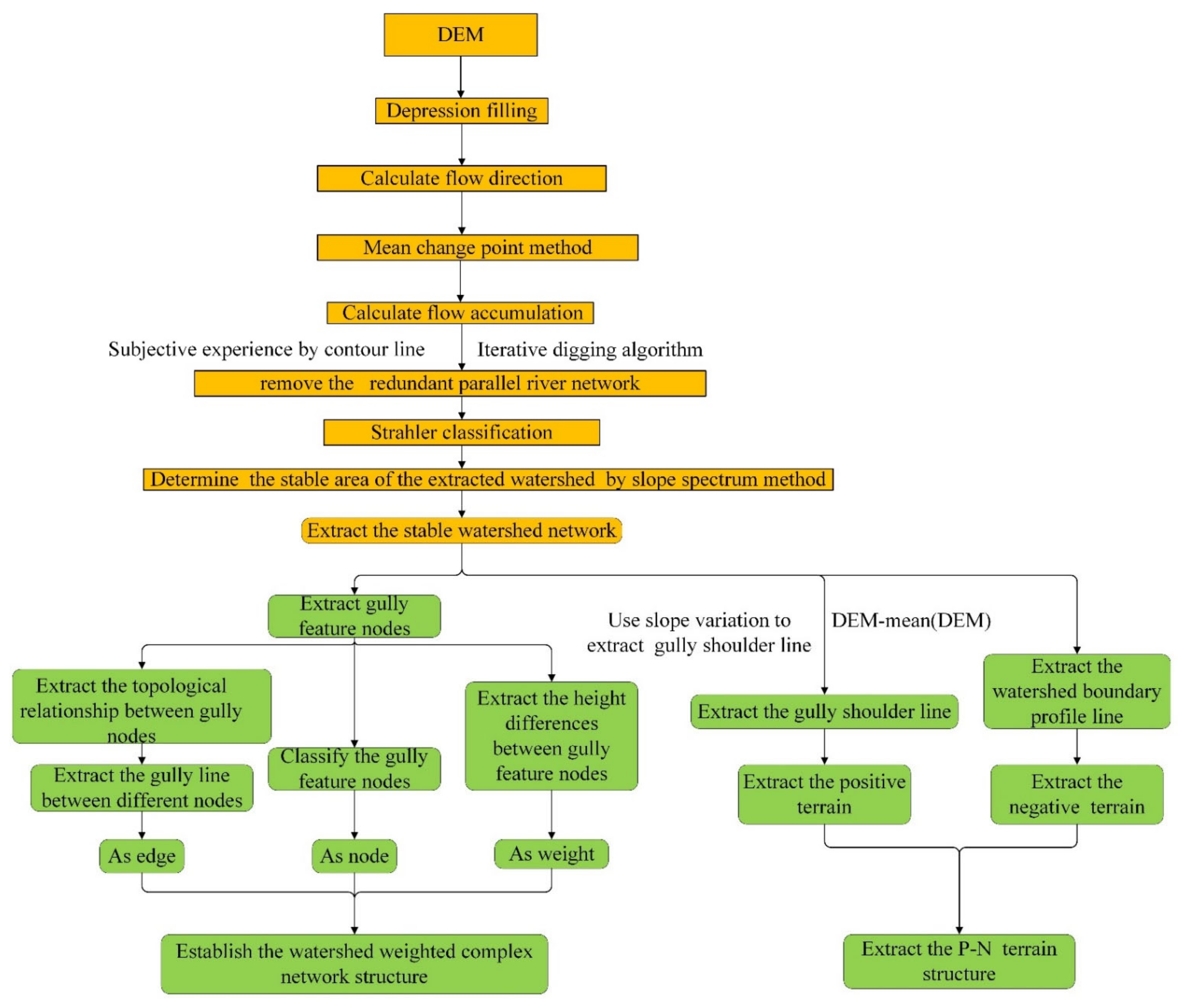
2. Materials and Methods

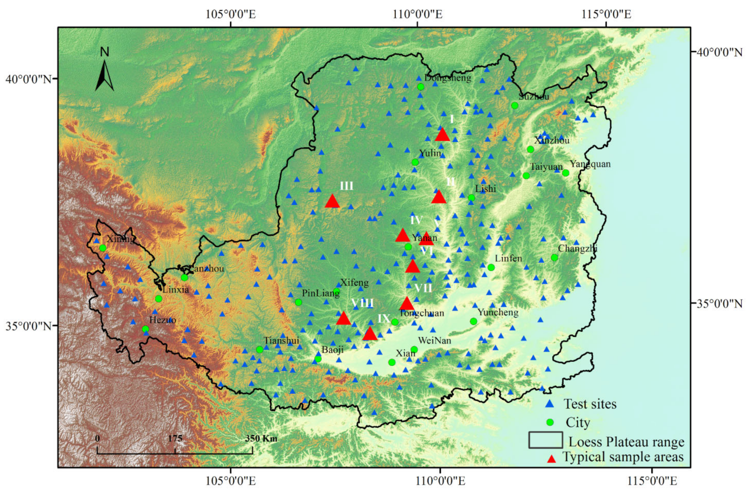
2.1. Materials

Loess Plateau, which is the most serious water and soil erosion area in the world, was chosen as the sample area herein (see Figure 1). With its unique geographical conditions, geomorphological research value, loess landform features, and natural and cultural landscapes, it has attracted worldwide attention [11,64]. The core landforms of the Loess Plateau are loess tableland, loess ridge, and loess hill. Simultaneously, stony mountains, sandhill, and valley plains are spread over the Loess Plateau. In terms of the six landforms, we extracted 300 loess watersheds randomly located in the Loess Plateau as the test sites. In terms of these test sites, 240 watersheds were randomly selected as the training datasets. To verify the accuracy and performance of the model based on the complex network methodology, 60 loess watersheds (ten watersheds for each landform type) were selected as the test dataset. Moreover, to compare the differences between the stable area with the divided area of the traditional method, nine sample areas were selected as the typical sample areas. These sample areas included nine typical loess landforms (see

Table 1. The typical sample area of nine loess landforms.

Area Name	Area Name	Center Latitude and Longitude	Landform Type	Development Stage
I	Shenmu	110°29′56.040″ N 38°50′32.424″ E	Loess deep incision gorge-hill	submature stage
II	Suide	110°18′45.000″ N 37°35′00.000″ E	Loess hill-ridge	late mature stage
III	Dingbian	107°35′52.548″ N 37°35′25.332″ E	Loess ridge-tableland	submature stage
IV	Ansai	109°21′00.000″ N 36°50′30.000″ E	Loess hill	late mature stage
V	Yanchuan	109°56′15.000″ N 36°45′00.000″ E	Loess hill-ridge	late mature stage
VI	Fuxian	109°33′45.000″ N 36°12′30.000″ E	Loess hill-ridge	late mature stage
VII	Yijun	109°22′30.000″ N 35°27′30.000″ E	Loess ridge	submature stage
VIII	Changwu	107°47′42.360″ N 35°12′24.120″ E	Loess tableland	infancy stage
IX	Chunhua	108°26′15.000″ N 34°52′30.000″ E	Loess middle-low mountain, loess platform-tableland	infancy stage

).

The data used in this paper were from an SRTM DEM that occupied the area from 60° N to 56° S captured by the Shuttle Radar Topography Mission (SRTM). The DEMs were resampled using the nearest neighbor method to be the DEMs with a resolution of 30 m × 30 m. To ensure the recognition landform types are unbiased, the landform types on the Loess Plateau referred to the Geographical zoning map provided by the Earth System Science Data Sharing Platform from 2000 (downloaded from http://www.geodata.cn/, accessed on 21 September 2021) and an investigation by Zhou [65].

2.2. Quantification of the Watershed Spatial Structure and Its Composition

To quantize the spatial structure and composition of the watershed, we adopted the complex network methodology and the positive–negative terrain theory to describe the watershed. The spatial structure for the loess watershed can be, respectively, simulated as the positive–negative terrain structure (Figure 2a) and the watershed network structure (Figure 2b). Figure 3 shows the technical route for constructing two kinds of watershed spatial structures.

The hydrological analysis is the common tool used in the watershed study. A series of common operations for watershed extraction from DEM data can be divided into the following four steps in order: (1) fill depression; (2) compute the flow direction; (3) compute the flow accumulation; (4) extract the catchment area by a certain threshold of the flow accumulation; and (5) classify the catchment area using the Strahler classification method [34,66]. The three key issues of extracting the stable watershed, respectively, are the determination of the reasonable flow accumulation threshold, the elimination of the error parallel stream, and the determination of the stable watershed area. The methods to solve these problems are given as follows [67,68].

To determine the reasonable flow accumulation threshold, the average variable point method is commonly used [69,70]. Gully density is an essential parameter that can not only reveal the evolutionary extent but also embody the solid erosion intensity [64]. With the increase in flow accumulation thresholds, a variable point in the slope of the gully density curve exists. The value of the variable point can be viewed as the suitable value that the watershed network tends to be stable [70,71]. The calculation of the variable point is as follows:

(1)

Gully densities under each flow accumulation threshold (100, 200, 300, …, 1000) were calculated to be a sequence [$\left\{{\mathrm{G}}_i\right\}$, $i=1,\cdots , \mathrm{N}$], where $\mathrm{i}$ is the number of $\mathrm{G}$. Then, we calculated the mean value of the sequence as $\overline{\mathrm{G}}$ and the deviation square sum for the sequence as $\mathrm{T}$.

(2)

The sequence of ${\mathrm{G}}_i$ can be divided into two sequences [{${ \mathrm{G}}_1$,${ \mathrm{G}}_k$}, {${ \mathrm{G}}_2$,${ \mathrm{G}}_{k-1}$}, … {${ \mathrm{G}}_{k-1}$,${ \mathrm{G}}_N$}]. ${\mathrm{T}}_k$ is obtained by adding the sum of deviation square between the two preceding samples and can be calculated using the following:

$${\mathrm{T}}_k={\displaystyle \sum }_{i=1}^{k-1}{\left({\mathrm{G}}_i-\overline{{\mathrm{G}}_{k1}}\right)}^2+{\displaystyle \sum }_{i=k}^{\mathrm{N}}{\left({\mathrm{G}}_i-\overline{{\mathrm{G}}_{k2}}\right)}^2$$

(1)

As seen in Figure 2, there is a variable point between the differences of ${\mathrm{T}}_k$ and $\mathrm{T}$ with the increase in the flow accumulation threshold. The variable point can be viewed as the suitable flow accumulation threshold [69,70].

The redundant parallel river networks are inevitable in the process of extracting watersheds. To eliminate the parallel river networks, the iterative digging algorithm, which is an effective method to reduce the height of the main ditch, was employed [68,72]. Ultimately, visual interpretation was conducted to further eliminate the remaining parallel river network as was possible based on the extracted contour line of the watershed (see Figure 4).

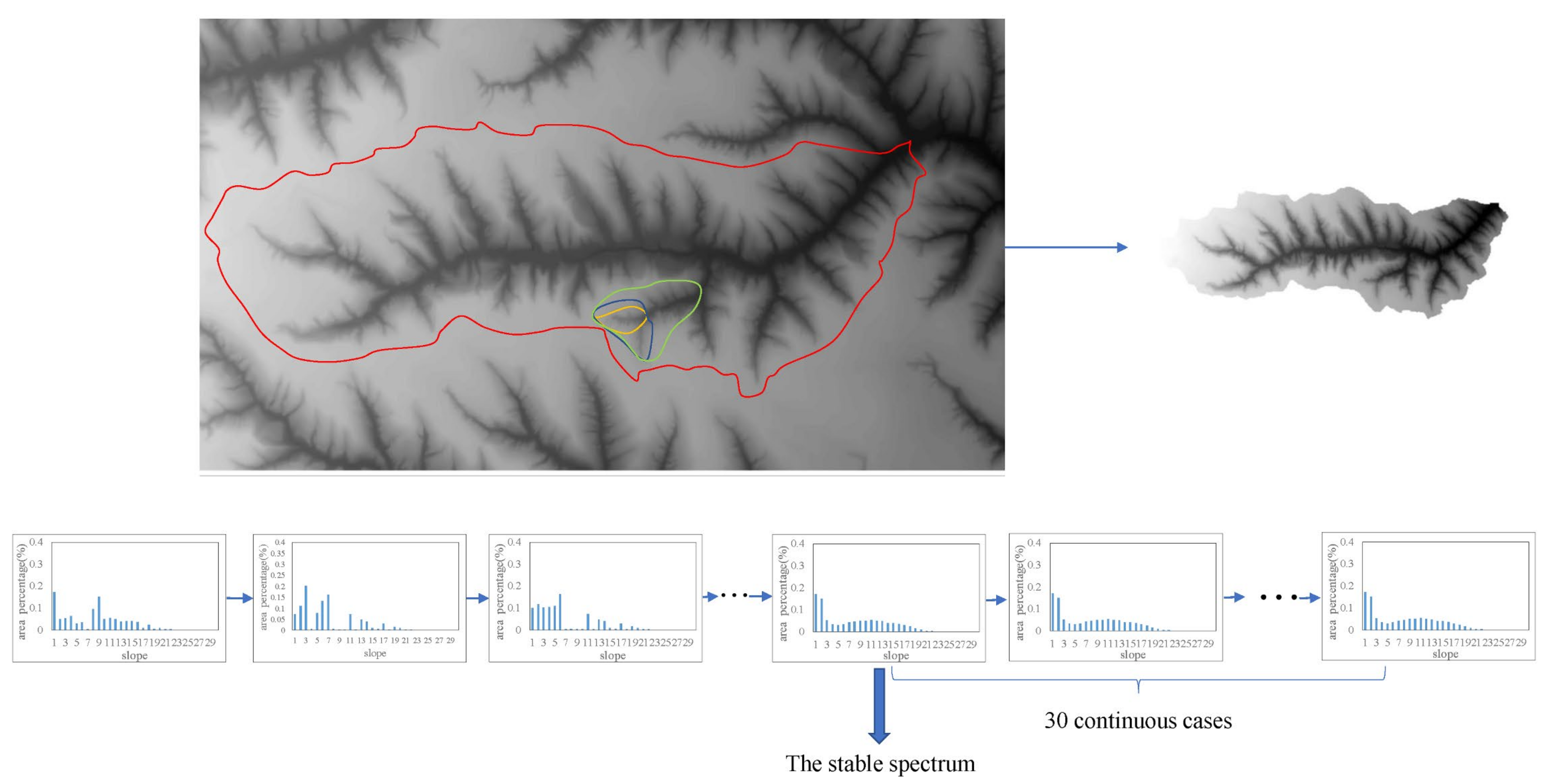
2.2.1. The Stable Watershed Area Based on the Slope Spectrum

The determination of watershed size is a factor of uncertainty in the field of watershed-based landform recognition. In previous studies, the watershed area is invariably determined by specifying a minimum value, which is adopted for all watershed units in the process of extracting watershed areas. We herein adopted the slope spectrum method to determine the stable area of each watershed unit.

The slope spectrum is an effective method for determining the stable spatial structure of landforms [28,37,73,74,75,76,77,78,79,80,81,82,83,84,85,86,87,88,89,90,91,92,93,94]. The combined features of slope (i.e., slope spectrum) is a quantitative characterization of the terrain spatial structure for the landform [81], which is closely related to geomorphic morphology and geomorphic development extent [83]. There exists a critical area that when the sampling area is greater than the threshold value, the slope spectrum contains sufficient terrain feature information representing the whole landform and, thus, presents stable combined features, and vice versa [82].

The spectra method that is widely used is mainly based on the expanding of an N* N analysis window. However, it is not suitable for the extraction of the critical area for the watershed since the watershed is an anisotropic terrain [64]. The calculation of spectral critical area based on catchment area is another effective method to determine the stable spatial structure of catchment units [64] (see Figure 5). As shown in Figure 6, initially, with the gradual expansion of the catchment area (from yellow to blue to green to red), the slope spectrum from the initial unstable state gradually becomes self-similar and stable. When the critical area (the area of the dotted box in the figure) was reached, the slope spectrum region was stable. The detailed calculation steps can be given as follows:

(1)

Calculate the slope map of the catchment area using the mesh-based clustering algorithm proposed by Zevenbergen [95].

(2)

Slope spectrums of different watershed units can be obtained by using overlap analysis. Slope classification with a 3 degrees equal-interval has been proven to be suitable for Loess Plateau [64,96], which was adopted in this paper.

(3)

The stability of the slope spectrum for the extracted watershed can be measured by the extracted slope spectrum with the referred slope spectrum. Defining the slope spectrum of the watershed before expanding as ${\mathrm{T}}_1=\left\{{\mathrm{t}}_{1,1},{ \mathrm{t}}_{1,2},{\mathrm{t}}_{1,3},{\mathrm{t}}_{1,\mathrm{i}},\dots ,{\mathrm{t}}_{1,30}\right\}$, where ${\mathrm{t}}_{1,\mathrm{i}}$ is the percentage of the area within the $\mathrm{i}$ slope class in the catchment area. Similarly, defining the slope spectrum of the watershed after expanding as ${\mathrm{T}}_2=\left\{{\mathrm{t}}_{2,1},{\mathrm{t}}_{2,2},{\mathrm{t}}_{2,3},{\mathrm{t}}_{2,\mathrm{i}},\dots ,{\mathrm{t}}_{1,30}\right\}$. Then, we defined the quantitative indices of similarity as ${\mathrm{E}}_1$ and ${\mathrm{E}}_2$, which take the forms ${\mathrm{E}}_1=\mathrm{Abs}\left(\mathrm{Max}({\mathrm{P}}_2)-\mathrm{Max}({\mathrm{P}}_1\right))$ and ${\mathrm{E}}_2=\sum _{\mathrm{i}=1}^{30}\mathrm{sum}\left(\mathrm{Abs} \left({\mathrm{P}}_{2,\mathrm{i}}-{\mathrm{P}}_{1,\mathrm{i}}\right)\right)$.

(4)

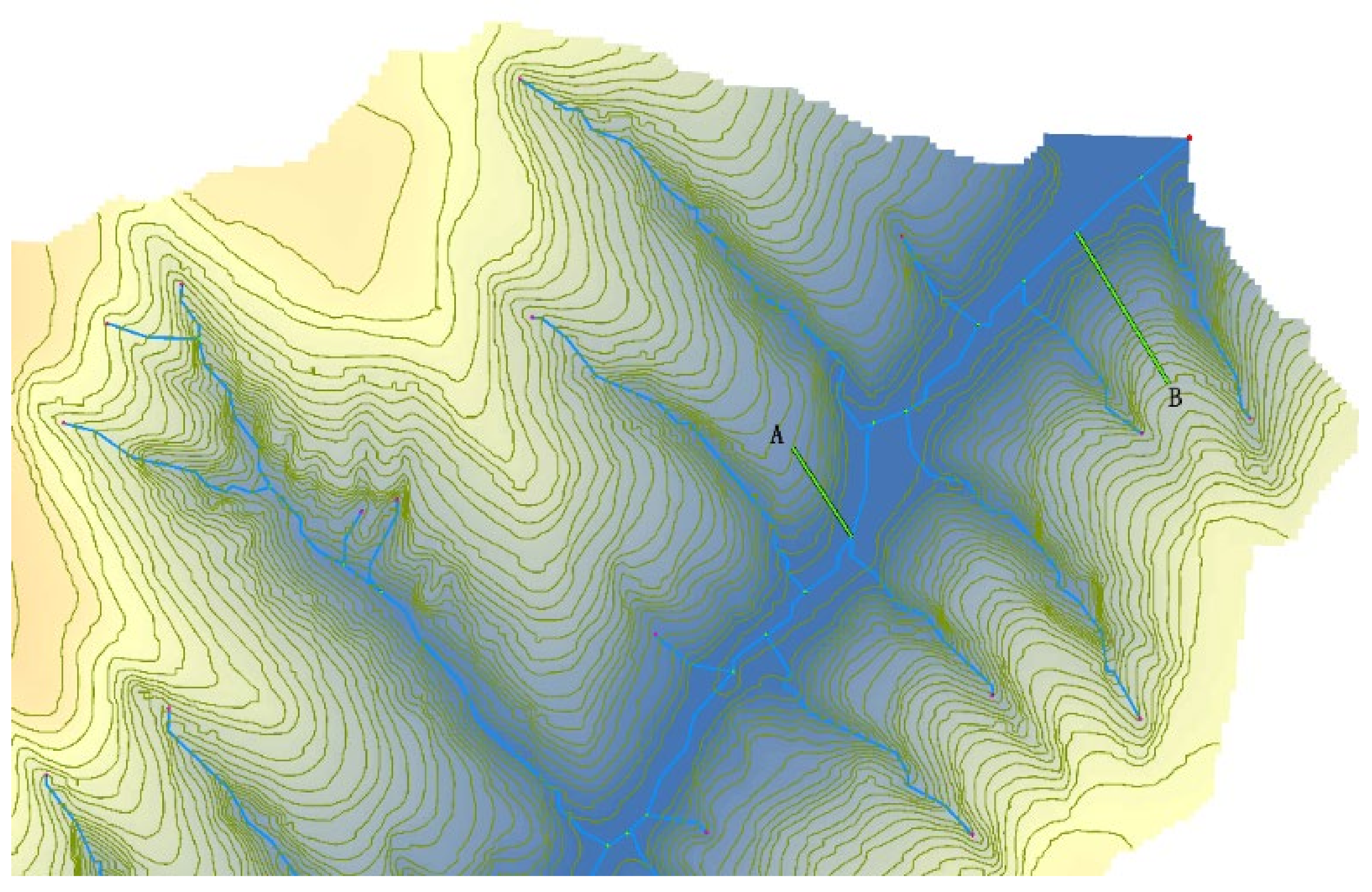
The watershed area continuously expanded by adding the new watershed unit to the catchment area. When there were 30 continuous cases where ${\mathrm{E}}_1<0.001$ and ${\mathrm{E}}_2<0.001$, we viewed ${\mathrm{P}}_1$ as the stable slope spectrum and the watershed area of the first case as the stable watershed area (see Figure 5).

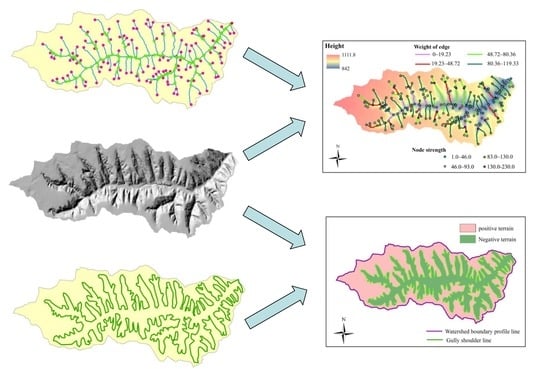
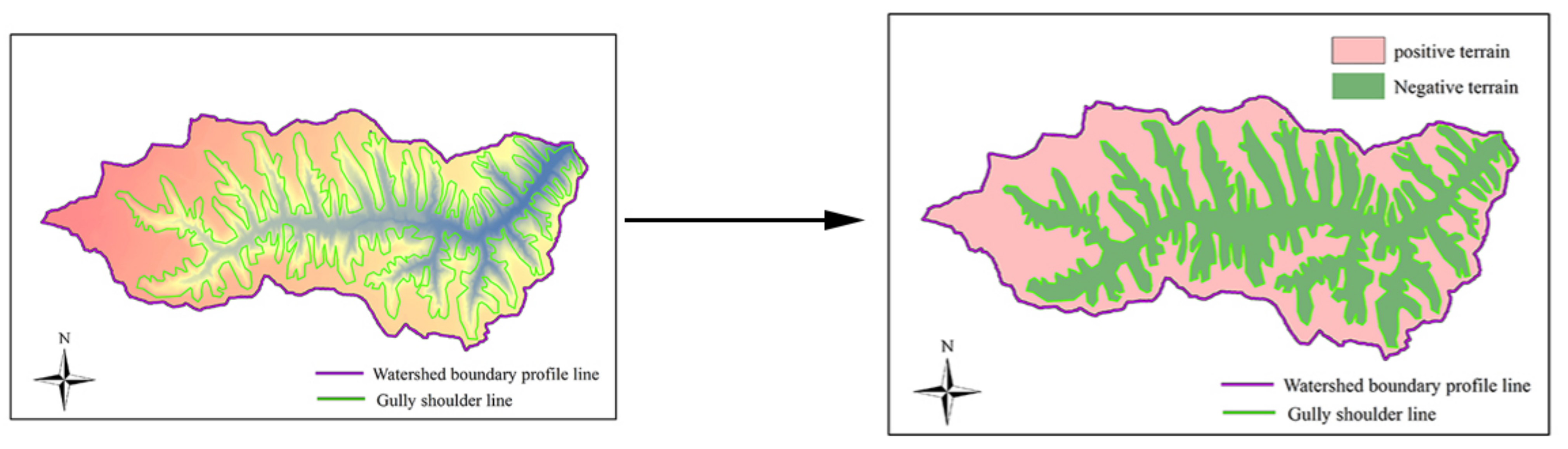
2.2.2. Extracting the P–N Spatial Structure of the Watershed

To extract the positive–negative (P–N) terrain, extracting the watershed boundary profile line and gully shoulder line is needed. The gully shoulder line can be extracted by combining the slope variation [97,98,99] and verified using the window smoothing method [100]. The watershed boundary profile line can be extracted by the scope extracting function of the ArcGIS. As the overall periphery of the catchment geomorphology, the watershed boundary line is the highest and the boundary line in the whole watershed, which is almost unaffected by the erosion of flowing water [101]. The Gully shoulder line is the important feature line that divides the positive and negative terrain in the loess watershed, which is also the boundary line of the soil erosion area and land utilization area [63]. Then, the P–N terrain can be further extracted by the division of the watershed boundary profile line and gully shoulder line (see Figure 6).

In the development process of the P–N terrain structure, on the one hand, with the continuous erosion by the severe water and gravity erosion, the positive terrain is gradually divided and nibbled away by the negative terrain, and the gully shoulder line gradually approached the watershed boundary profile line. On the other hand, the energy and material are in the process of mutual migration and transformation. These lead to the result that there are huge differences in the internal topographic features of the P–N terrain in different landform types. The relationship of composition between the P–N terrain is one of the five basic relationships in geomorphic classification [102]. The spatial structures of the P–N terrain are the marks for distinguishing different landform types.

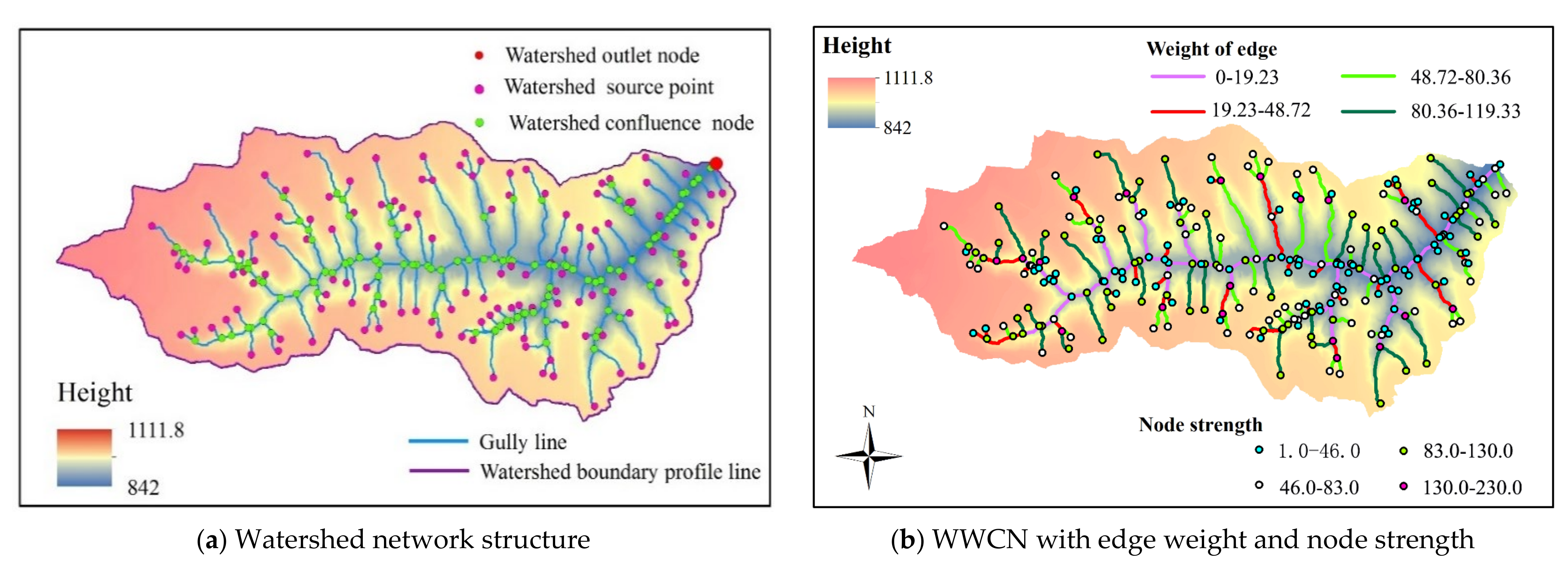
2.2.3. Extracting the WWCN Spatial Structure of the Watershed

The process to extract the gully feature nodes and connectivity relations between different nodes can be given in the following steps: (1) extract the watershed feature node layer via establishing stream network dataset; (2) extract watershed feature nodes possessing confluence level information through spatial join function of ArcGIS; and (3) obtain connectivity relation between different nodes through the spatial query.

To derive the weight further (i.e., the height differences of the interconnecting watershed feature nodes), the following procedures were adopted. Firstly, we obtained the watershed connecting edge element by attribute query. Then, to extract height differences between the watershed feature nodes that are connected, overlay analysis of ArcGIS was conducted between the watershed connecting edge elements and the corresponding watershed unit. For each watershed edge, the height difference between the watershed feature nodes that it linked was viewed as the weight for it.

Nodes, edges, and weight are the basic three elements for constructing the weight complex network. From the respect of complex network theory, a watershed can be viewed as the gully spatial structure that is made up of a series of watershed feature nodes connected by gullies [67,103]. The types of watershed feature nodes can be divided into the watershed outlet node, the watershed source point, and the watershed confluence node (see Figure 7a).To construct the watershed weighted complex network (called WWCN for short), we herein defined the watershed feature nodes as the network nodes and defined the topological connection (gullies) between the neighboring watershed feature nodes as the network edge, and defined the height differences between the neighboring nodes as the weight of the edge.

The red points are the watershed outlet points, which are the outlets of the watershed and are the points with the lowest height as well as the largest flow amount in the watershed. The pink points are the watershed source nodes, the source of the watershed. The green points are the watershed confluence nodes, which are the intersect nodes between different streams. The gully nodes are not only different in form and quantity, but also have a strong combination of spatial relations, forming an orderly whole through a mutual connection. As seen in Figure 7b, following the topological relation of the simulated WWCN spatial structure, each node and edge were given their unique attribute value (i.e., node strength and edge weight).

2.2.4. The Quantitative Description of the WWCN Spatial Structure and P–N Terrain Spatial Structure

Combining the complex network theory and the watershed geomorphology, the gully line density, average node strength, fractal dimension, structure entropy, average path length, network density, and modularity were proposed to quantitatively describe the WWCN spatial structure (see

Table 2. The quantitative indexes of WWCN spatial structure and their corresponding algorithm.

Quantitative Indexes	Algorithm	Remark
Average node strength (NS)	$N{S}_i=\frac{{{\displaystyle \sum }}_{i=1}^N\left({{\displaystyle \sum }}_{j\in N_i}{a}_{ij}{w}_{ij}\right)}{N}$	$w_{ij}$ is the edge weight (height differences) between node $i$ and node $j$; $a_{ij}$ is the element of the network adjacency matrix
Average path length (AL)	$AL=\frac{1}{\frac{1}{2}n\left(n-1\right)}{\displaystyle {\displaystyle \sum }_{i>j}}{d}_{ij}$	$n$ is the total number of the nodes in the network;$d_{ij}$ is the distance between node $i$ and node j (i.e., the sum number of edges in the shortest path of two nodes);
Fractal dimension (FD)	$d=-lim\frac{\ln t\left(r\right)}{ln r}$	Box dimension method is a common and effective approach [104]. For any watershed network, we used the box whose length is r to cover it. We computed the number of nonempty boxes (t(r)) with the case that watershed under setting different lengths (r = 1, 2, 3, 4, …, M). By defining r as the x-axis and $\ln t\left(r\right)$ as the y-axis, least-square method was utilized to conduct linear regression. The negative slope for the fitted equation is the fractal dimension.
structure entropy (SE)	$H_i=\frac{d\left(i\right)}{{{\displaystyle \sum }}_{i=1}^{n}d\left(i\right)};SE=-{\displaystyle {\displaystyle \sum }_{i=1}^n}{H}_{i}ln{H}_i$	$H_i$ is the importance of i-th node; $n$ is the total number of the network node; $d\left(i\right)$ is the degree of the i-th node.
network density (ND)	$d\left(G\right)=2m/\left[n\left(n-1\right)\right]$	m is the actual number of connected edges in the network; $n$ is the sum number of the nodes;
Modularity (M)	$M=\frac{1}{2m}{\displaystyle {\displaystyle \sum }_{i,j}}(A_{ij}-k_i{k}_j/\left(2m\right)\delta \left(C_i,C_j\right)$	$m$ is the total edges of the network; $k_i$ is the sum of the weights for node $i$; $A_{ij}$ represents the weight of the edge between node $i$ and node $i$;$\delta \left(a,b\right)$ is the function that set $\delta$ = 1 when a = b, otherwise $\delta$ = 0;$C_i$ is the community to which node $i$ belonged.
gully line density	$GL=\frac{L}{A}$	GL is the gully line density, $L$ is the total length of the gully lines in the sample area, $A$ is the watershed area.

). According to the P–N spatial structure, Extent for nibbling away ($\mathit{EN}$), Cutting Depth ($C_d$), Shape Metrics ($S_d$), Homogeneous index ($H$), Fragmentation ($F$), and Mean-Slope-Difference ($\mathit{MSD}$) were proposed to quantitatively depict the P–N terrain spatial structure (see

Table 3. The quantitative indexes of P–N terrain spatial structure and their corresponding algorithms.

Quantitative Indexes	Algorithm	Remark
Extent for nibbling away ($EN$)	$EN=\frac{S_n}{S_p}$	$S_a$ is the horizontal projection area of the negative terrain; $S_b$ is the horizontal projection area of the positive terrain
Cutting Depth ($C_d$)	$C_d=Mean\left(H_p\right)-Mean\left(H_n\right)$	$H_p$ is the height of the positive terrain; $H_n$ is the height of the negative terrain;
Shape Metrics ($S_d$)	$S_d={\displaystyle {\displaystyle \sum }_{i=1}^N}{W}_i\frac{L_i}{2\sqrt{\pi S_i} }$	$S_d$ is the shape metric; $W_i$ is area weight of the $i$-th patch; $S_i$ is area of the $i$-th patch; $L_i$ is the perimeter of the $i$-th patch
Homogeneous index ($H$)	$H=\sqrt{\frac{{\sum }_{i=1}^N {\left[A_i-\left({\sum }_{i=1}^n{A}_i/n\right)\right]}^2}{N}\ast {10}^6}$	$n$ is the number of positive patch; $A_i$ is the area of each positive patch;
Fragmentation ($F$)	$F=\frac{n}{{{\displaystyle \sum }}_{i=1}^N A_i}$	$n$ is the number of positive patch; $A_i$ is the area of each positive patch;
Mean-Slope-Difference ($MSD$)	$MSD=Mean\left(S_p\right)-Mean\left(S_n\right)$	$S_p$ is the slope of the positive terrain; $S_n$ is the slope of the negative terrain;

).

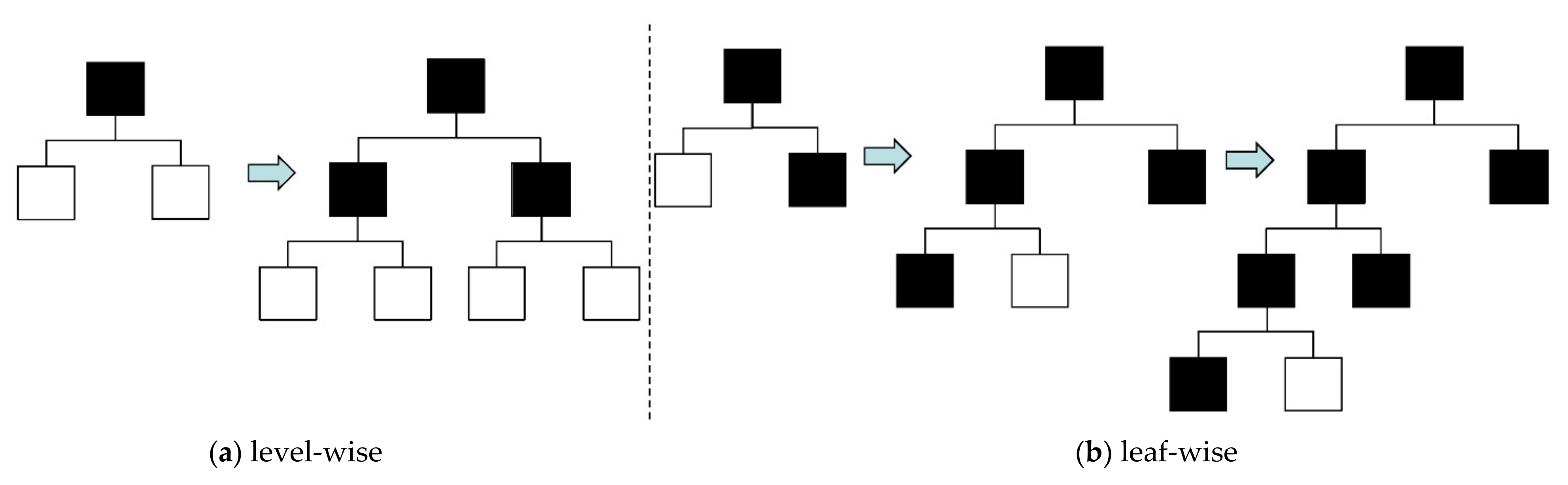
2.3. Light Gradient Boosting Machine

LightGBM (Light Gradient Boosting Machine) is a new gradient Boosting Decision tree frame with high efficiency, fast training speed, and distributed support [105]. Since its good performance in different machine learning tasks such as sorting, classification, and regression, it has been widely employed in different academic fields [105,106,107,108]. However, its application on landform auto-classification is rare, though it has shown enough potential in landform application. Thus, this paper adopted it to conduct the loess landform auto-classification.

Two key differences between it and other gradient boosting tree algorithms were the histogram-based algorithms in the search of split points (see Figure 8) and the leaf-wise tree growth strategy with depth limit (see Figure 9). The basic idea of the histogram algorithm is to discretize the continuous feature values into K integers and a histogram of K bins can be constructed by that. By traversing the data, the discretized values are used as indexes to accumulate statistics in the histogram. After traversing the data once, the required statistics were accumulated in the histogram. According to the discrete value of the histogram, the optimal split points can be found. Since the number of the bins were less than the data amount, compared to the presorting algorithm used by another gradient boosting tree algorithm, the time complexity, and memory footprint of the histogram algorithm dramatically decreased. That is, the root node is determined first, and then the branches are determined according to the information gain and other indicators. The structure of the tree is formed by analogy.

Alternatively, in the direction of tree growth, the general decision tree algorithm adopts the level-wise method (see Figure 9a). That is, the root node is determined first and the branches are divided indiscriminately. However, many branches of low gains are unnecessary. Differently, the leaf-wise tree growth strategy was adopted in the LightGBM. In each branch, the leaf with the largest gain was found from all the current branches, then split (see Figure 9b). The strategy will circulate constantly. Therefore, when the trees are increased to the same branch, the algorithm based on leaf-wise strategy may decrease more errors and obtain more accuracy. However, when sample data are little, leaf-wise may lead to overfitting. Based on this, the depth-limit parameter can limit the depth of trees to avoid overfitting.

2.4. Evaluation Criterion and Experimental Design

The recall rate, precision, F1 values, and confusion matrix are the basic evaluation metrics in classification based on machine learning, which is extensively used. For one landform type, precision measures the ratio of correct classification results to the classification results. For one landform type, recall rate refers to the ratio of correct classified landform numbers to the actual landform numbers. To comprehensively estimate the classification performance for one landform type, the F1 value is the mean of the recall rate and the precision. The confusion matrix is a statistic table produced by the actual landform types and the landform classification result, which is generally used to analyze the errors and confusion of the landform classification results.

Moreover, overall accuracy and Kappa coefficient are adopted to comprehensively evaluate the overall performance of the landform classification result. The overall accuracy is the proportion of correctly classified samples to total samples. Kappa coefficient denotes the ratio of error reduction in classification to a completely random classification. It can be given by the following:

$$Kappa=\frac{P{\sum }_{i=1}^n{T}_{ii}-{\sum }_{i=1}^n{T}_{i+}{T}_{+i}}{P^2-{\sum }_{i=1}^m{T}_{i+}x{T}_{+i}}$$

(2)

where $P$ is the sample number, m is the total number of the classes, $T_{ii}$ is the number of the correctly classified samples, $T_{i+}$ is the classified sample number of the i-th class, and $T_{+i}$ is the total sample number of the i-th class.

The dataset was divided into the training dataset and test dataset by the ratio of 8:2. To prevent the problem of overfitting, five folds cross validation was conducted in the training datasets. Moreover, based on the five folds cross validation, grid search was employed to find the optimal model. Grid search is a method to find the optimal parameters of the machine learning methods [109,110]. It is an algorithm that calculates the parameters of the function by cross validation, in the form of the permutations and combinations for the possible values of each parameter. Although the grid search is time-consuming, it has a wide search range and is likely to find the optimal parameter combination.

3. Results and Discussions

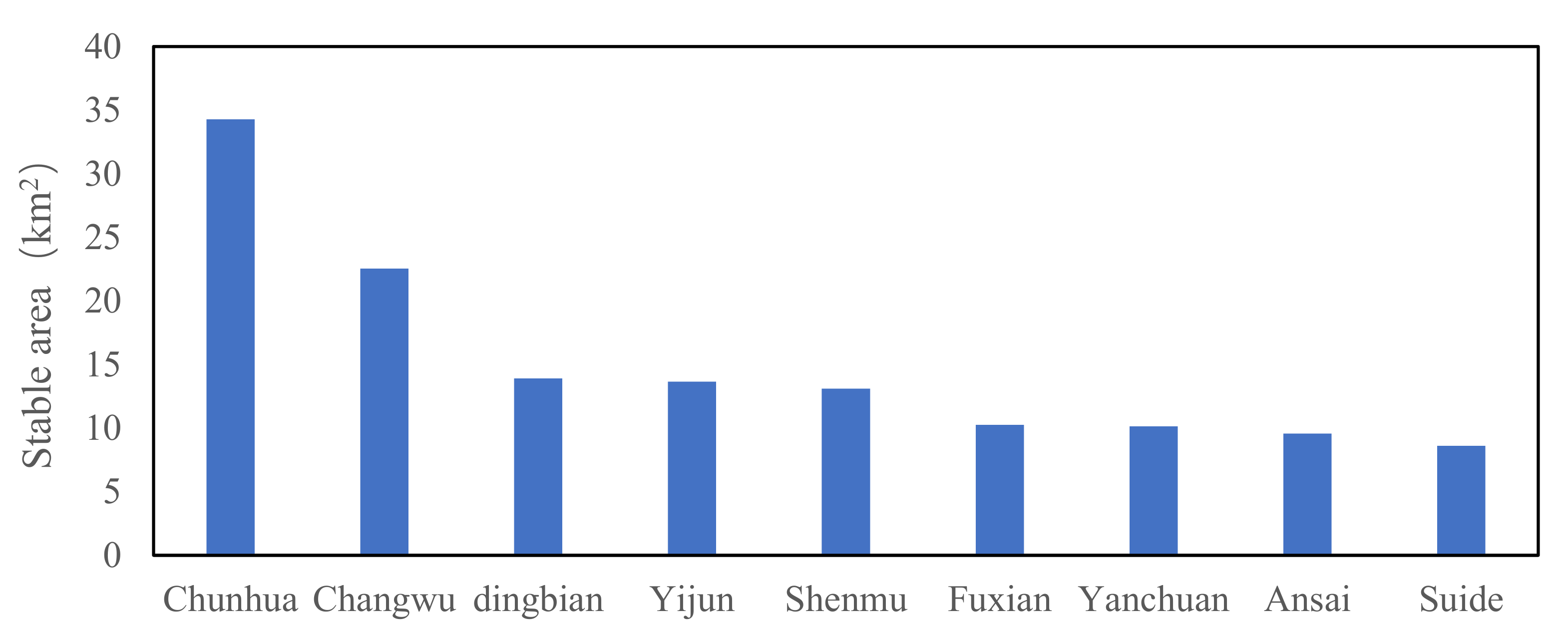
3.1. The Stable Area of the Watershed

The stable area of the watershed unit for different landforms is different. Previous scholars generally control the size of each watershed unit at a uniform value, such as 10 [27,28], 30 [88], and 100 km² [61]. A segmentation area of a watershed that is too small may mean that the watershed cannot fully contain the terrain features of the sample area and, thus, affect the recognition accuracy. Values that are too large may contain the “noise signals” of the terrain and bring heavy work for the studiers. Thus, slope spectrum, which is an effective method to determine the landform spatial structure, was adopted in this paper to control the size of the watershed unit.

To investigate the stable area of the extracted watershed, we used the slope spectrum method to extract the stable area of the nine typical loess landforms (see Figure 10). We ranged the size of the watershed stable areas to find the laws. Combining Table 1 and Figure 10, the watershed showed a regular descending trend with the landform evolution. The more evolution the loess terrain is, the lower the size of the stable area is. The reasons for that can be explained as follows. For the landforms in high evolution, the landform features are complex and, thus, obvious. Only a small watershed area is needed to present the whole terrain’s features. It was consistent with the regularity of “the more complex the loess terrain is, the lower stable area will be” [64]. On the other hand, the different landform types generally showed different watershed stable areas. Most of the stable watershed area was around 10 km², which corresponded to the stable area determination of previous scholars [27,28]. However, for the 300 watersheds, the size of the stable area that was between 10–15 km² accounted for only 63.33%. It suggested that the uniform stable area for all the watersheds is unsuitable; the stable watershed areas for some regional landform sites are not around 10 km².

Obviously, with a uniform value of 30 or 10 km², it may be suitable for most of the areas. However, there will always be some watershed units whose stable area is greater than the fixed value. It can be noted that the stable watershed areas of the 300 watersheds were all less than 100 km². The uniform value of 100 km² is superfluous, which brings too much work for researchers. Thus, the method of determining the stable area via slope spectrum may be better than the traditional method of determining by unifying the watershed area.

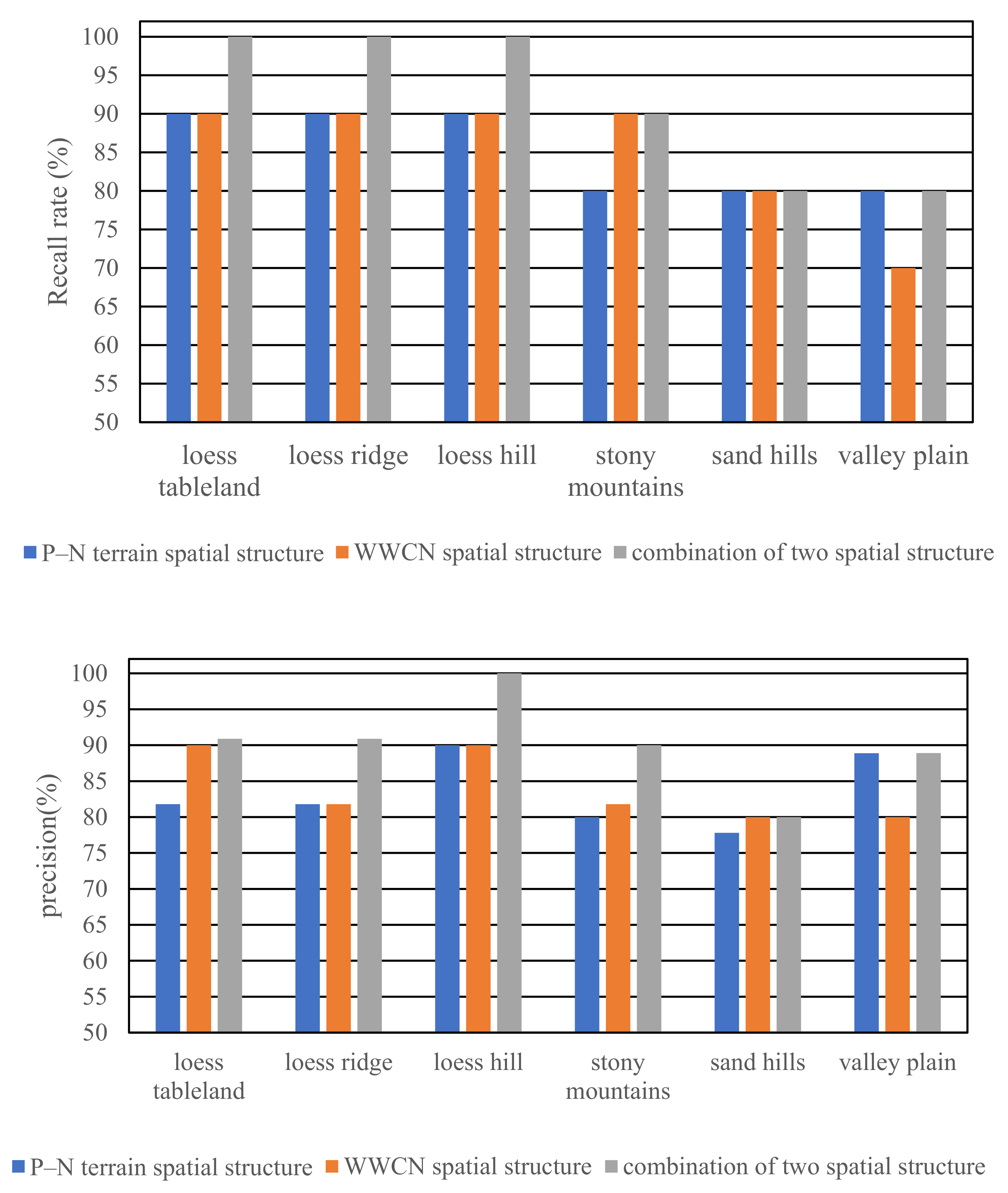
3.2. Recognition Result Based on Different Watershed Spatial Structures

Based on the watershed stable area of different sites, we extracted the corresponding watersheds. Then, we first constructed the P–N terrain spatial structure and the WWCN spatial structure to extract the 13 comprehensive quantitative indexes as the feature matrix. A total of 240 watersheds were taken as the training datasets to construct the classified model via the LightGBM and the remaining 60 watersheds were adopted as the test datasets to verify the recognition effect. A grid search with cross validation was conducted to construct the basic LightGBM model. Via the LightGBM model, we, respectively, conducted the landform recognition based on the single spatial structure and the combination of the two spatial structures.

To comprehensively compare the performances between these three classification methods, Figure 11 shows the recall rate and precision of these three classification results. As can be seen in Figure 11, most of the recall rates and precision are beyond 80%, which suggests the good performance of these two landform recognition methods. These indicated that by depicting the terrain spatial structure of the landform from different angles, the WWCN spatial structure and the P–N terrain spatial structure are feasible for the classification of landforms. The accuracy and recall rate of the P–N terrain spatial structure is generally lower than that based on the WWCN spatial structure. Moreover, for the WWCN spatial structure, the overall accuracy is 85% and the kappa coefficient is 0.82; for the P–N terrain spatial structure, the overall accuracy is 83.333% and the kappa coefficient is 0.80066. Thus, for the single quantitative description of the watershed spatial structure, the WWCN spatial structure exhibited a better identification effect than the P–N terrain spatial structure.

It was noted that although for most landform types, the performances of the WWCN-based recognition are better than the P–N terrain-based classification, the recognition result of the recall rate and precision for valley plain are reverse to the other results. This result indicated that the valley plain is not easy to distinguish based on the angle of the WWCN terrain spatial structure due to its flat and wide terrain. In this case, the P–N terrain theory provided another better angle for the quantitative description of the landform spatial structure. Moreover, for the landform of obvious spatial structure, the P–N terrain-based methods and the WWCN-based methods all showed good performance. In terms of the recall rate, the loess tableland, loess ridge, and loess hill all reached 90%, whereas the sandhill and valley plain are lower. The same phenomenon can be observed in the F1 values, the loess tableland, loess ridge, and loess hill, which also reached higher values than the other three landform types. The much-developed ravines and the broken landform surface of typical loess landforms led to the obvious spatial structure. Adversely, with slight terrain relief, sand hill and valley plain were full of sand or plain and the terrains were flat. It may suggest that the quantitative description method via considering the spatial structure has a positive response to the landform types with an obvious spatial structure such as loess hill and loess ridge. Another evidence is that when we combine the two spatial structures to conduct the landform recognition, the F1 values of the loess typical landforms (loess tableland, loess ridge, loess hill) all increased and were greater than the sand hill and valley plain.

Table 4. The confusion matrix produced by combining the WWCN spatial structure and the P–N terrain spatial structure.

	Loess Tableland	Loess Ridge	Loess Hill	Stony Mountain	Sand Hill	Valley Plain	Precision (%)	Recall Rate (%)	F1 (%)
Loess tableland	10	0	0	0	0	0	90.9	100	95.45
Loess ridge	0	10	0	0	0	0	90.9	100	95.45
Loess hill	0	0	10	0	0	0	100	100	100
Stony mountain	0	1	0	9	0	0	90	90	90
sand hill	1	0	0	0	8	1	80	80	80
valley plain	0	0	0	0	2	8	88.9	80	84.45
	Overall accuracy, 91.67%
	Kappa coefficient, 0.9004

shows the confusion matrix of the recognition result based on the combination of these two structures. The recall rate and precision generally increased. The F1 values all have a certain increase. The overall accuracy reached 91.67% and the Kappa coefficient reached 0.9004. By contrast, the classified result (Figure 12a) fitted well with the actual results (Figure 12b). It suggested that the recognition performance of the data fusion schemes of two watershed spatial structures is greater than the other two methods. This also indicated that the quantitative description of the WWCN spatial structure and that of the P–N terrain spatial structure are complementary. Combining the data of quantitative description for the WWCN spatial structure and that for the P–N terrain spatial structure can significantly improve the geomorphic recognition ability.

One finding to be noted is that the distinction between loess ridge and loess mound is successful. However, differing loess ridge from loess hill was generally difficult [24]. The morphology of the two landform types are similar, and their definitions are ambiguous, making the classification difficult. The proposed method may provide a good approach for distinguishing the two kinds of landform types.

We can observe that the greatest confusion was in the sand hill, valley plain, and the loess tableland, which may be attributed to the presence of similar patterns between the relatively flat landforms. In these landforms, the terrains suffering from weaker erosion were, thus, in low evolution. For the relatively smooth and unbroken terrain, compared to loess hill or loess ridge with the rough topography and great relief intensity, the spatial structure or morphology may be similar or inconspicuous, thereby being difficult to distinguish.

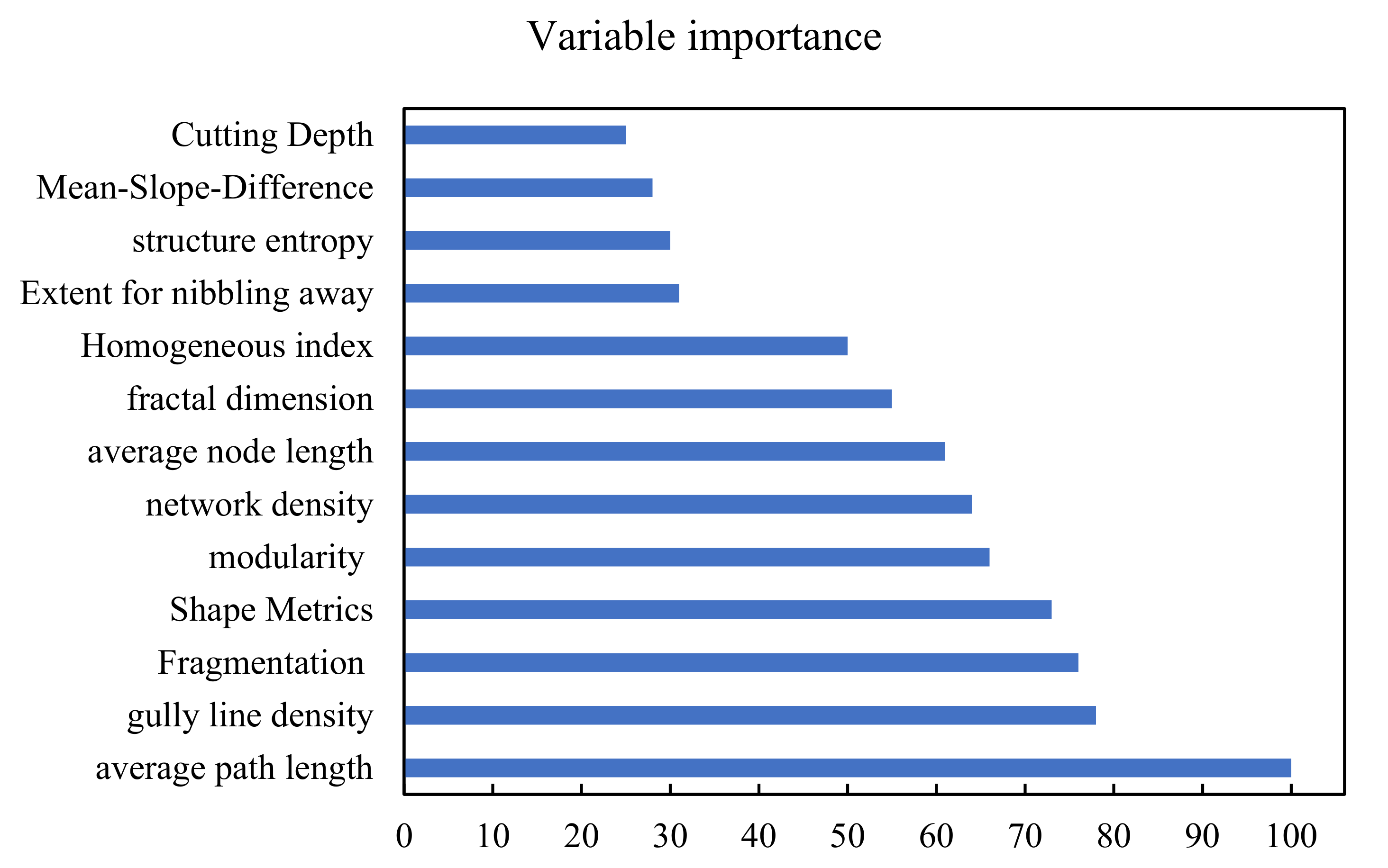
3.3. Importances of Different Comprehensive Quantitative Indexes

The LightGBM based on the machine learning database of python offers a series of simple internal measures to estimate the importance of employed feature variables. In this paper, the importance of the feature variables can reflect the quantitative description extent of the feature variable to the watershed spatial structure. Figure 13 shows the importance of the different feature variables.

The importance of most WWCN indices was greater than the importance of the P–N terrain indices. It may suggest that the contribution of the WWCN indices was greater than the P–N terrain indices in the landform recognition process. The finding may explain the result that the recognition performance based on the quantitative description of the WWCN spatial structure is worse than that based on the quantitative description of the P–N terrain spatial structure.

Furthermore, we observed that the parameters that were closely related to the combined watershed structure (such as the average node strength, gully line density, fragmentation, network density, etc.) were, generally, at the relative front of the order of importance. These indices were closely related to the basic combination of the watershed structure, which is the gullies, gully nodes, P–N patches, etc. The finding proved that the basic combination of the watershed spatial structure has good explanatory power for the landform recognition, which is, to some extent, strong support for the study base in this paper.

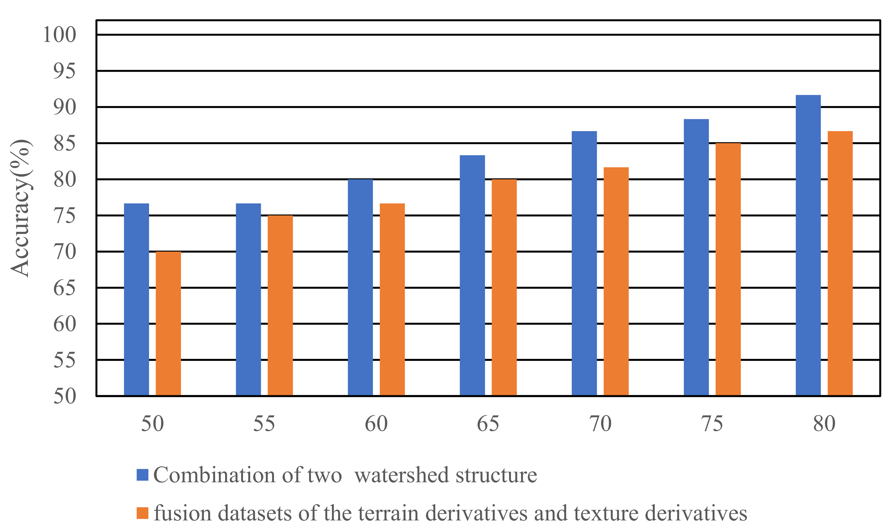
3.4. Comparison with the Fusion of Terrain Derivatives and Texture Derivatives

Previous scholars invariably recognized landforms by extracting terrain derivatives and texture derivatives. To compare the landform recognition by the combination of the two spatial structures with the landform recognition based on the terrain derivatives and texture derivatives, thirteen quantitative indices were extracted from the 300 watersheds as the terrain feature datasets. These quantitative indices were the terrain derivatives or texture derivatives, which have been found to be of high importance in landform recognition by previous investigations [13]. A grid search with cross validation was also conducted to construct the optimum LightGBM model.

Table 5. The confusion matrix produced by the fusion datasets of the terrain derivatives and texture derivatives. Noted that the fusion datasets included average slope, variance of slope, variance of curvature, entropy of slope, average slope of slope, elevation range, hillshading entropy, slope entropy, elevation variance, standard deviation of slope of slope, standard deviation of curvature, hillshading contrast, and the maximum slope.

	Loess Tableland	Loess Ridge	Loess Hill	Stony Mountain	Sand Hill	Valley Plain	Precision (%)	Recall Rate (%)	F1 (%)
Loess tableland	9	1	0	0	1	0	90	90	90
Loess ridge	1	8	1	0	0	0	66.67	80	73.34
Loess hill	0	2	8	0	0	0	88.89	80	84.45
Stony mountain	0	1	0	9	0	0	90	90	90
sand hill	1	0	0	0	8	1	88.89	80	84.4
valley plain	0	0	0	1	0	9	90	90	90
	Overall accuracy, 86.67%
	Kappa coefficient, 0.8404

shows the confusion matrix based on the fusion datasets of the terrain derivatives and texture derivatives. The kappa coefficient is 0.8404 and the overall accuracy is 86.67%, which showed that the recognition effect is worse than the recognition effect based on the combination of the two watershed structures.

In terms of the landform types, the F1 values of loess hill and loess ridge were relatively lower, which corresponds to the findings of Zhao [13]. On the contrary, the F1 values of valley plain and stony mountain were greater than that based on the combination of the two watershed structures. This may indicate valley plain and stony mountain have relatively obvious terrain features and texture features. On the other hand, the proposed method can be complementary to the previous methods.

Several experiments were conducted to further evaluate the differences in the landform recognition methods. Specifically, we took 50, 55, 60, 65, 70, 75, and 80% of the sample datasets as the training datasets and the remaining datasets as the test datasets. Based on these dataset’s division, the landform recognitions were, respectively, conducted to study how the number of training samples affects the recognition accuracy [10,111]. Figure 14 shows the results using two kinds of methods in terms of different training–test ratios. Furthermore, in different dataset divisions, the accuracies of the proposed method were generally greater than the accuracies based on the fusion datasets of the terrain derivatives and texture derivatives. The recognition accuracies based on different methods were regularly enhanced with the increase in training datasets. Moreover, the mean increase in the accuracy of the proposed method is about 2.5%, whilst the accuracy increase in the previous method is about 2%. It suggested that the proposed method is more robust.

3.5. Comparison with Other Popular Machine Learning Methods

To quantitatively evaluate the performance of the LightGBM, the proposed method was compared with the other three popular machine learning methods (Random forest (RF), Extreme Gradient Boosting algorithm (XGBoost), Gradient-boosted decision trees (GBDT), support vector machine (SVM)). To fairly compare the recognition performance, the ratio of training datasets to the test datasets was in line with that based on the LightGBM. A grid search with five folds cross validation was performed to find the optimum model of the different machine learning methods.

Under different machine learning methods,

Table 6. Comparisons between the five kinds of machine learning methods. The bold number represents the greatest values in each column.

	Loess Tableland	Loess Ridge	Loess Hill	Stony Mountain	Sand Hill	Valley Plain	Total Accuracy
LightGBM	95.45	95.45	100	90	80	84.45	91.67
RF	95	90	90	90	80	84.44	88.34
XGBoost	95.45	90.91	95	90	90	84.45	90
GBDT	90	90	90	84.44	85.91	80	86.67
SVM	90	85.91	90	90	85.91	80.00	86.67

shows the F1 values of different landforms and the total accuracy. It is not difficult to find that for different machine learning algorithms, the landform recognition based on the combination of the two watershed structures generally showed good performances. All of the total accuracies were greater than 80%. It can be noted that the recognition effect of XGBoost, whose total accuracy reaches 90%, nearly weighs against XGBoost. However, the time consumption of XGBoost is often several times greater than that of the LightGBM [106,112,113]. The LightGBM is a better choice when the recognition accuracy of both is similar. Meanwhile, we observed that the F1 values of the proposed method outperform all the other algorithms for all the six landform types. Thus, we can conclude that the LightGBM based on the combination of the two watershed structures is an effective method with high accuracy in conducting landform recognition.

3.6. Innovations of This Study

Watershed-based landform recognition has been a new spot in the field of landform classification. However, there are still some unexplored but significant bottlenecks in this field.

Firstly, the divided small watershed area must ensure the property stability of the small watershed [37]. The extracted area size of the watershed must ensure the property stability of the watershed. Previous scholars generally employed a uniform sized area of the watershed to extract each watershed. However, for different landforms, the stable spatial structure area of the watershed is different [114]. When the area size of the extracted watershed is small, the watershed is unstable; therefore the terrain indices derived from the watershed cannot represent the overall landform type [27,29,115,116,117]. In this paper, the slope spectrum method is used to extract the stable area of the watershed, which provides a new insight for solving this issue.

Secondly, traditional landform recognition methods mainly rely on basic terrain derivatives and texture derivatives such as slope, elevation, hillshading, and other terrain factors [29,36,38,118,119]. The watershed object-based landform recognition method also relies on the original method’s system used in previous studies. Thus far, there is no basic theory that is separated from the original method of the landform recognition system.

Based on this, we, for the first time, proposed an effective methodology to conduct landform recognition from the perspective of the watershed spatial structure. In terms of the watershed, the spatial structure is diverse, complex, and dynamic. As an effective method for a quantitative description of a spatial structure [44,59,119], the complex network method has not been used in landform recognition based on watershed units. The P–N terrain theory is also a common and effective method in landform demarcation for the landform spatial structure. Thus, a series of carefully designed experiments were conducted on the 300 watersheds of the Loess Plateau to extract the P–N terrain and the WWCN for simulating the watershed spatial structure. Then, a series of quantitative indices were proposed to quantify the spatial structure and composition of the watershed from multiple angles. Via the LightGBM, we found that the simulation and quantification of the watershed spatial structure can effectively recognize the geomorphology with high accuracy. Thus, the proposed method provides new methodology and insights for landform recognition in the field of using watersheds as a basic unit.

By contrast, for the combination of two kinds of watershed spatial structures, the comprehensive performance was better than that based on the basic terrain derivatives and texture derivatives in the landform recognition on Loess Plateau. Furthermore, the proposed method possesses better robustness. It is noted that in the previous loess landform studies, the recognition of the loess hill and loess ridge is generally difficult due to its complex but similar morphology. Indeed, even for some terrain experts, it is not easy to identify. However, by combining the WWCN spatial structure and the P–N terrain structure to conduct the landform recognition, the performance is good and outperformed that based on basic terrain indices. It may suggest that, except for not being inferior to the inherent landform recognition methods based on the terrain factor, the proposed method is more effective than the previous methods in some landforms where the spatial structure or morphology is complex.

Moreover, in comparison with other popular machine learning methods, we investigated the adaptation of the watershed structure-based approach to the LightGBM. The experiments’ result showed that the combination of the LightGBM and the watershed structure-based approach achieved the greatest comprehensive performance, which provided references for upcoming research.

3.7. Possible Limitations

The quantification of the watershed is inevitably affected by DEM resolution. It may lead to local feature error, which will affect the classification accuracy. However, this is an unavoidable problem for digital terrain analysis based on DEM.

We compared the proposed method with the method based on the basic terrain indices and proved its good performance. However, further improvements are possible, e.g., can the proposed method be further combined with a method based on the basic terrain indices? This is a valuable but difficult theme that can be further explored. Due to the limitation of the paper content, this paper focus on exploring the potential of the proposed method in the field of landform classification using watershed as a basic unit.

4. Conclusions

This paper firstly proposed a landform recognition method from the view of the watershed spatial structure and composition. The methodology combines the WWCN and P–N terrain to simulate and quantify the watershed spatial structure, which breaks out the fixed theory of landform recognition based on the terrain indices. The proposed method showed convincing performance on the landform recognition to the six landform types. The observation and conclusion can be given as follows:

(1)

The watershed structure-based method is an effective landform recognition theory with rich potential in the landform recognition field of using the watershed as a basic unit. The fusion of the WWCN spatial structure and the P–N terrain structure can significantly improve the landform recognition performance. It is noted that the WWCN is the first attempt of the complex network theory in the landform recognition field.

(2)

Without using a uniform area as a criterion for watershed area division, the slope spectrum method is used to determine the stable area of the watershed. It provides additional insights for the area determination of the watershed.

(3)

The landform recognition performance and robustness based on the combination of the WWCN and P–N terrain outperformed that based on the terrain derivatives and texture derivatives, thereby suggesting the great significance of our study.

(4)

The methods from the angle of the watershed spatial structure and composition seemed to be well adapted to some similar or complex landforms. The loess ridge and loess hill are generally difficult to distinguish via landform recognition or artificial discrimination. The proposed method is effective in alleviating the confusion of the two kinds of similar landforms. By adopting the combination of the WWCN and P–N terrain to simulate the watershed spatial structure, the F1 values reached 95.4% and 100%, respectively, which was better than the method based on the basic terrain indices.

(5)

The LightGBM algorithm is suitable to be employed for the landform recognition of the watershed structure-based method since it showed better performance than the other machine learning methods.

In brief, the proposed method, from the view of the watershed spatial structure and composition, is a new methodology differing from the previous method that fairly relies on the terrain indices. It further provides additional insights and enriches the theory for the landform recognition field of using the watershed as a basic unit.

References

1. Mokarram, M.; Sathyamoorthy, D. A review of landform classification methods. Spat. Inf. Res. 2018, 26, 647–660. [Google Scholar] [CrossRef]
2. Moreno, M.; Levachkine, S.; Torres, M.; Quintero, R. Landform classification in raster geo-images. In Progress in Pattern Recognition, Image Analysis and Applications; Sanfeliu, A., Trinidad, J.F.M., Ochoa, J.A.C., Eds.; Lecture Notes in Computer Science; Springer: Berlin, Germany, 2004; Volume 3287, pp. 558–565. [Google Scholar]
3. Wang, Y.; Qin, C. Review of automatic classification methods for geomorphic morphological types. Geogr. Geo Inf. Sci. 2017, 33, 16–21. [Google Scholar]
4. Kilic Gul, F. Geomorphometry-Automatic Landform Classification. J. Geogr. Cograf. Derg. 2018, 36, 15–26. [Google Scholar] [CrossRef] [Green Version]
5. Wang, D.; Laffan, S.W.; Liu, Y.; Wu, L. Morphometric characterisation of landform from DEMs. Int. J. Geogr. Inf. Sci. 2010, 24, 305–326. [Google Scholar] [CrossRef] [Green Version]
6. Evans, I.S. Geomorphometry and landform mapping: What is a landform? Geomorphology 2012, 137, 94–106. [Google Scholar] [CrossRef]
7. Jasiewicz, J.; Stepinski, T.F. Geomorphons—A pattern recognition approach to classification and mapping of landforms. Geomorphology 2013, 182, 147–156. [Google Scholar] [CrossRef]
8. Hiller, J.; Smith, M. Residual relief separation: Digital elevation model enhancement for geomorphological mapping. Earth Surf. Process. Landf. 2008, 33, 2266–2276. [Google Scholar] [CrossRef] [Green Version]
9. Drăguţ, L.; Blaschke, T. Automated classification of landform elements using object-based image analysis. Geomorphology 2006, 81, 330–344. [Google Scholar] [CrossRef]
10. Du, L.; You, X.; Li, K.; Meng, L.; Cheng, G.; Xiong, L.; Wang, G. Multi-modal deep learning for landform recognition. ISPRS J. Photogramm. Remote Sens. 2019, 158, 63–75. [Google Scholar] [CrossRef]
11. Xiong, L.; Tang, G.; Yang, X.; Li, F. Geomorphology-oriented digital terrain analysis: Progress and perspectives. J. Geogr. Sci. 2021, 31, 456–476. [Google Scholar] [CrossRef]
12. Burrough, P.A.; van Gaans, P.F.; MacMillan, R. High-resolution landform classification using fuzzy k-means. Fuzzy Sets Syst. 2000, 113, 37–52. [Google Scholar] [CrossRef]
13. Zhao, W.-F.; Xiong, L.-Y.; Ding, H.; Tang, G.-A. Automatic recognition of loess landforms using Random Forest method. J. Mt. Sci. 2017, 14, 885–897. [Google Scholar] [CrossRef]
14. Tribe, A. Automated recognition of valley heads from digital elevation models. Earth Surf. Process. Landf. 1991, 16, 33–49. [Google Scholar] [CrossRef]
15. Bishop, M.P.; James, L.A.; Shroder, J.F., Jr.; Walsh, S.J. Geospatial technologies and digital geomorphological mapping: Concepts, issues and research. J. Geomorphol. 2012, 137, 5–26. [Google Scholar] [CrossRef]
16. Hammond, E.H. Analysis of properties in land form geography: An application to broad-scale land form mapping. Ann. Assoc. Am. Geogr. 1964, 54, 11–19. [Google Scholar] [CrossRef]
17. MacMillan, R.A.; Pettapiece, W.W.; Nolan, S.C.; Goddard, T.W. A generic procedure for automatically segmenting landforms into landform elements using DEMs, heuristic rules and fuzzy logic. Fuzzy Sets Syst. 2000, 113, 81–109. [Google Scholar] [CrossRef]
18. Saha, K.; Wells, N.A.; Munro-Stasiuk, M. An object-oriented approach to automated landform mapping: A case study of drumlins. Comput. Geosci. 2011, 37, 1324–1336. [Google Scholar] [CrossRef]
19. Smith, M.J. Digital Mapping: Visualisation, interpretation and quantification of landforms. In Developments in Earth Surface Processes; Elsevier: Amsterdam, The Netherlands, 2011; Volume 15, pp. 225–251. [Google Scholar]
20. Stepinski, T.F.; Ghosh, S.; Vilalta, R. Automatic recognition of landforms on Mars using terrain segmentation and classification. In Proceedings of the International Conference on Discovery Science, Barcelona, Spain, 7–10 October 2006; pp. 255–266. [Google Scholar]
21. Migoń, P.; Woo, K.-S.; KaSprzaK, M. Landform recognition in granite mountains in East Asia (Seoraksan, Republic of Korea, and Huangshan and Sanqingshan, China)—A contribution of geomorphology to the UNESCO World Heritage. Quaest. Geogr. 2018, 37, 103–115. [Google Scholar] [CrossRef] [Green Version]
22. Kasprzak, M.; Jancewicz, K.; Różycka, M.; Kotwicka, W.; Migoń, P. Geomorphology-and geophysics-based recognition of stages of deep-seated slope deformation (Sudetes, SW Poland). Eng. Geol. 2019, 260, 105230. [Google Scholar] [CrossRef]
23. Yang, X.; Tang, G.; Meng, X.; Xiong, L. Classification of Karst Fenglin and Fengcong Landform Units Based on Spatial Relations of Terrain Feature Points from DEMs. Remote Sens. 2019, 11, 1950. [Google Scholar] [CrossRef] [Green Version]
24. Li, S.; Xiong, L.; Tang, G.; Strobl, J. Deep learning-based approach for landform classification from integrated data sources of digital elevation model and imagery. Geomorphology 2020, 354, 107045. [Google Scholar] [CrossRef]
25. Zhou, X.; Xie, X.; Xue, Y.; Xue, B.; Qin, K.; Dai, W. Bag of Geomorphological Words: A Framework for Integrating Terrain Features and Semantics to Support Landform Object Recognition from High-Resolution Digital Elevation Models. ISPRS Int. J. Geo-Inf. 2020, 9, 620. [Google Scholar] [CrossRef]
26. Janušaitė, R.; Jukna, L.; Jarmalavičius, D.; Pupienis, D.; Žilinskas, G. A Novel GIS-Based Approach for Automated Detection of Nearshore Sandbar Morphological Characteristics in Optical Satellite Imagery. Remote Sens. 2021, 13, 2233. [Google Scholar] [CrossRef]
27. Xiong, L.-Y.; Zhu, A.-X.; Zhang, L.; Tang, G.-A. Drainage basin object-based method for regional-scale landform classification: A case study of loess area in China. Phys. Geogr. 2018, 39, 523–541. [Google Scholar] [CrossRef]
28. Cao, Z.; Fang, Z.; Yao, J.; Xiong, L.I. Study on loess landform classification based on random forest. J. Geo Inf. Sci. 2020, 22, 452–463. [Google Scholar]
29. Verhagen, P.; Drăguţ, L. Object-based landform delineation and classification from DEMs for archaeological predictive mapping. J. Archaeol. Sci. 2012, 39, 698–703. [Google Scholar] [CrossRef]
30. Drăguţ, L.; Eisank, C. Object representations at multiple scales from digital elevation models. Geomorphology 2011, 129, 183–189. [Google Scholar] [CrossRef] [Green Version]
31. Blaschke, T. Object based image analysis for remote sensing. ISPRS J. Photogramm. Remote Sens. 2010, 65, 2–16. [Google Scholar] [CrossRef] [Green Version]
32. Blaschke, T.; Hay, G.J.; Kelly, M.; Lang, S.; Hofmann, P.; Addink, E.; Feitosa, R.Q.; Van der Meer, F.; Van der Werff, H.; Van Coillie, F. Geographic object-based image analysis–towards a new paradigm. ISPRS J. Photogramm. Remote Sens. 2014, 87, 180–191. [Google Scholar] [CrossRef] [Green Version]
33. Chen, G.; Weng, Q.; Hay, G.J.; He, Y. Geographic object-based image analysis (GEOBIA): Emerging trends and future opportunities. GIScience Remote. Sens. 2018, 55, 159–182. [Google Scholar] [CrossRef]
34. Strahler, A.N. Quantitative analysis of watershed geomorphology. Eos Trans. Am. Geophys. Union 1957, 38, 913–920. [Google Scholar] [CrossRef] [Green Version]
35. Cao, M.; Tang, G.a.; Zhang, F.; Yang, J. A cellular automata model for simulating the evolution of positive–negative terrains in a small loess watershed. Int. J. Geogr. Inf. Sci. 2013, 27, 1349–1363. [Google Scholar] [CrossRef]
36. Huang, S.-L.; Ferng, J.-J. Applied land classification for surface water quality management: II. Land process classification. J. Environ. Manag. 1990, 31, 127–141. [Google Scholar] [CrossRef]
37. Wang, L.; Zhou, Y. Study on the classification of typical loess geomorphology facing sub-basin units. Arid Zone Res. 2019, 36, 1592–1598. [Google Scholar]
38. Caratti, J.F.; Nesser, J.A.; Lee Maynard, C. Watershed classification using canonical correspondence analysis and clustering techniques: A cautionary note 1. J. Am. Water Resour. Assoc. 2004, 40, 1257–1268. [Google Scholar] [CrossRef]
39. Monteiro, F.C.; Campilho, A. Watershed framework to region-based image segmentation. In Proceedings of the 2008 19th International Conference on Pattern Recognition, Tampa, FL, USA, 8–11 December 2008; pp. 1–4. [Google Scholar]
40. Zuecco, G.; Rinderer, M.; Penna, D.; Borga, M.; Van Meerveld, H. Quantification of subsurface hydrologic connectivity in four headwater catchments using graph theory. Sci. Total Environ. 2019, 646, 1265–1280. [Google Scholar] [CrossRef]
41. Rong, J.; Pan, Y.L. Accuracy improvement of graph-cut image segmentation by using watershed. Adv. Mater. Res. 2012, 341, 546–549. [Google Scholar] [CrossRef]
42. Pirzada, S.; Dharwadker, A. Applications of graph theory. J. Korean Soc. Ind. Appl. Math. 2007, 7, 2070013. [Google Scholar]
43. Phillips, J.D.; Schwanghart, W.; Heckmann, T. Graph theory in the geosciences. Earth Sci. Rev. 2015, 143, 147–160. [Google Scholar] [CrossRef]
44. Strogatz, S.H. Exploring complex networks. Nature 2001, 410, 268–276. [Google Scholar] [CrossRef] [Green Version]
45. Poulter, B.; Goodall, J.L.; Halpin, P.N. Applications of network analysis for adaptive management of artificial drainage systems in landscapes vulnerable to sea level rise. J. Hydrol. 2008, 357, 207–217. [Google Scholar] [CrossRef]
46. Abe, S.; Suzuki, N. Complex-network description of seismicity. Nonlinear Process. Geophys. 2006, 13, 145–150. [Google Scholar] [CrossRef]
47. Tian, Z.; Jia, L.m.; Dong, H.h.; Su, F.; Zhang, Z.D. Analysis of Urban Road Traffic Network Based on Complex Network. Procedia Eng. 2016, 137, 537–546. [Google Scholar] [CrossRef] [Green Version]
48. Yu, F.; Xue, L.; Sun, C.; Zhang, C. Product transportation distance based supplier selection in sustainable supply chain network. J. Clean. Prod. 2016, 137, 29–39. [Google Scholar] [CrossRef]
49. Hossmann, T.; Spyropoulos, T.; Legendre, F. A complex network analysis of human mobility. In Proceedings of the 2011 IEEE Conference on Computer Communications Workshops, Shanghai, China, 10–15 April 2011; pp. 876–881. [Google Scholar]
50. Kaluza, P.; Kölzsch, A.; Gastner, M.T.; Blasius, B. The complex network of global cargo ship movements. J. Royal Soc. Interface 2010, 7, 1093–1103. [Google Scholar] [CrossRef]
51. Lin, J.; Ban, Y. Complex network topology of transportation systems. Transp. Rev. 2013, 33, 658–685. [Google Scholar] [CrossRef]
52. Prabakaran, G.; Vaithiyanathan, D.; Ganesan, M. Application of fuzzy combined SVM & graph theory for agriculture productivity prediction. J. Phys. Conf. Ser. 2020, 1706, 012039. [Google Scholar]
53. Cantwell, M.D.; Forman, R.T. Landscape graphs: Ecological modeling with graph theory to detect configurations common to diverse landscapes. Landsc. Ecol. 1993, 8, 239–255. [Google Scholar] [CrossRef]
54. Wu, X.; Yu, K.; Wang, X. On the growth of Internet application flows: A complex network perspective. In Proceedings of the 2011 IEEE INFOCOM, Shanghai, China, 10–15 April 2011; pp. 2096–2104. [Google Scholar]
55. Gan, C.; Yang, X.; Liu, W.; Zhu, Q.; Jin, J.; He, L. Propagation of computer virus both across the Internet and external computers: A complex-network approach. Commun. Nonlinear Sci. Numer. Simul. 2014, 19, 2785–2792. [Google Scholar] [CrossRef]
56. Heckmann, T.; Schwanghart, W.; Phillips, J.D. Graph theory—Recent developments of its application in geomorphology. Geomorphology 2015, 243, 130–146. [Google Scholar] [CrossRef]
57. Beauguitte, L.; Ducruet, C. Scale-free and small-world networks in geographical research: A critical examination. In Proceedings of the 17th European Colloquium on Theoretical and Quantitative Geography, Athens, Greece, 1 September 2011; pp. 663–671. [Google Scholar]
58. Suweis, S.; Konar, M.; Dalin, C.; Hanasaki, N.; Rinaldo, A.; Rodriguez-Iturbe, I. Structure and controls of the global virtual water trade network. Geophys. Res. Lett. 2011, 38, L10403. [Google Scholar] [CrossRef] [Green Version]
59. Halverson, M.J.; Fleming, S.W. Complex network theory, streamflow, and hydrometric monitoring system design. Hydrol. Earth Syst. Sci. 2015, 19, 3301–3318. [Google Scholar] [CrossRef] [Green Version]
60. Rinaldo, A.; Banavar, J.R.; Maritan, A. Trees, networks, and hydrology. Water Resour. Res. 2006, 42, W06D07. [Google Scholar] [CrossRef]
61. Zhou, Y.; Yang, X.; Xiao, C.; Zhang, Y.; Luo, M. Positive and negative terrains on northern Shaanxi Loess Plateau. J. Geogr. Sci. 2010, 20, 64–76. [Google Scholar] [CrossRef]
62. Xiong, L.; Tang, G.; Yan, S.; Zhu, S.; Sun, Y. Landform-oriented flow-routing algorithm for the dual-structure loess terrain based on digital elevation models. Hydrol. Process. 2014, 28, 1756–1766. [Google Scholar] [CrossRef]
63. Yang, F.; Zhou, Y. Quantifying spatial scale of positive and negative terrains pattern at watershed-scale: Case in soil and water conservation region on Loess Plateau. J. Mt. Sci. 2017, 14, 1642–1654. [Google Scholar] [CrossRef]
64. Tang, G.; Song, X.; Li, F.; Zhang, Y.; Xiong, L. Slope spectrum critical area and its spatial variation in the Loess Plateau of China. J. Geogr. Sci. 2015, 25, 1452–1466. [Google Scholar] [CrossRef] [Green Version]
65. Zhou, Y. Study on Positive and Negative Topography and Spatial Differentiation of Loess Plateau Based on DEM. Ph.D. Thesis, Nanjing Normal University, Nanjing, China, 2011. [Google Scholar]
66. Strahler, A.N. Quantitative slope analysis. Geol. Soc. Am. Bull. 1956, 67, 571–596. [Google Scholar] [CrossRef]
67. Zhu, H.; Zhao, Y.; Xu, Y.; Liu, H. Hierarchy structure characteristics analysis for the China Loess watersheds based on gully node calibration. J. Mt. Sci. 2018, 15, 2637–2650. [Google Scholar] [CrossRef]
68. Li, C.; Li, F.; Dai, Z.; Yang, X.; Cui, X.; Luo, L. Spatial variation of gully development in the loess plateau of China based on the morphological perspective. Earth Sci. Inform. 2020, 13, 1103–1117. [Google Scholar] [CrossRef]
69. Wang, K.; Chen, N. Extraction method for terrain feature point considering spatial feature. Sci. Surv. Mapp. 2021, 46, 192–202. [Google Scholar]
70. Lai, H.; Bing, X.; Liang, H.; Bi, X.; Yang, Z.; Lu, J. Extraction of River Network in Three Gorges Reservoir Area Based on Mean Change Point Analysis. Sci. Surv. Mapp. 2012, 37, 173–175. [Google Scholar]
71. Tucker, G.E.; Bras, R.L. Hillslope processes, drainage density, and landscape morphology. Water Resour. Res. 1998, 34, 2751–2764. [Google Scholar] [CrossRef] [Green Version]
72. Wang, T. A Preliminary Study on Population Characteristics of Gullies in Small Watershed of the Loess Plateau. Doctoral Dissertation, Nanjing Normal University, Nanjing, China, 2015. [Google Scholar]
73. Zhu, M.; Li, F. Study on the influence of slope classification on surface slope spectrum. Sci. Surv. Mapp. 2009, 34, 165–167. [Google Scholar]
74. Dang, X.; Zhou, C.; Wang, B.; Wei, W. Evolution of slope spectrum of construction land in China and influence of slope climbing. Acta Geogr. Sin. 2021, 76, 1747–1762. [Google Scholar]
75. Yang, Q.; Wang, C. Study on minimum area threshold for slope statistical analysis. Sci. Surv. Mapp. 2020, 45, 172–177. [Google Scholar]
76. Zhao, W.; Dong, Q.; Yan, T.; Qin, W.; Zhu, Q. Analysis of the relationship between slope spectrum information entropy and topographic factors in purple soil water erosion area in southwest China. Trans. Chin. Soc. Agric. Eng. 2020, 36, 160–167. [Google Scholar]
77. Zhao, M.; Tang, G.; Chen, Z.; Zhu, H.C. Comparison of different slope classification systems and surface slope spectrum in loess hilly and gully region. Bull. Soil Water Conserv. 2002, 33–36. [Google Scholar]
78. Yi, X.; Zhou, F.; Wang, X.; Yang, Y.; Guo, H. Watershed classification and runoff simulation in no data area based on SOM. Progress Geogr. 2014, 33, 1109–1116. [Google Scholar]
79. Wu, S.; Rao, L. Characteristics and spatial differentiation of slope spectrum in different types of arsenic sandstone. Trans. Chin. Soc. Agric. Eng. 2021, 37, 125–132. [Google Scholar]
80. Tang, G. Exploration and Practice of Digital Terrain Analysis on Loess Plateau; Science Press: Beijing, China, 2015. [Google Scholar]
81. Wang, C.; Tang, G.; Li, F.; Zhu, X.; Jia, Y. Uncertainty of slope spectrum information extraction based on DEM. Geoinf. Sci. 2008, 10, 539–544. [Google Scholar] [CrossRef]
82. Wang, C.; Tang, G.; Li, F.; Yang, X.; Ge, S. Basic regional conditions for extraction and application of slope spectrum. Sci. Geogr. Sin. 2007, 27, 587–592. [Google Scholar]
83. Tang, G.; Zhao, M.; Li, T.; Liu, Y.; Xie, Y. Uncertainty of ground slope in loess Plateau extracted from DEM. Acta Geogr. Sin. 2003, 58, 824–830. [Google Scholar]
84. Li, F.; Tang, G.; Wang, C.; Cui, L.; Zhu, R. Slope spectrum variation in a simulated loess watershed. Front. Earth Sci. 2016, 10, 328–339. [Google Scholar] [CrossRef]
85. Tang, G.; Na, J.; Cheng, W. Research progress of digital topographic analysis of regional geomorphology in China. Acta Geod. Et Cartogr. Sin. 2017, 46, 1570–1591. [Google Scholar]
86. Tang, G.; Li, F. Xiong LI-yang. Research progress of digital topographic analysis on loess Plateau. Geogr. Geo Inf. Sci. 2017, 33, 1–7. [Google Scholar]
87. Peng, Q.; Tang, L.; Chen, J.; Chen, Y. Study on slope spectrum evolution of construction land in Shenzhen in 2000 and 2015. J. Nat. Resour. 2018, 33, 2200–2212. [Google Scholar]
88. Liu, S.; Li, F.; Jiang, R.; Chang, R.; Liu, W. Automatic identification and analysis of slope spectrum of loess landform types. J. Geo Inf. Sci. 2015, 17, 1234–1242. [Google Scholar]
89. Li, H.; Wu, J.; Wang, X. Object-oriented land use classification in Dongjiang River Basin based on GF-1 image. Trans. Chin. Soc. Agric. Eng. 2018, 34, 245–252. [Google Scholar]
90. Li, F.; Tang, G.; Jia, P.; Cao, Z. Scale effect and spatial differentiation of slope spectrum information entropy. Geoinf. Sci. 2007, 9, 13–18. [Google Scholar] [CrossRef]
91. Ju, Z.; Zhang, J.; Bai, Z. Study on the relationship between information entropy of mountain slope spectrum and topographic factors of soil and water loss. Sci. Surv. Mapp. 2019, 44, 86–90. [Google Scholar]
92. Chu, Y.; Zhu, L.; Tang, B.; Li, X. Characteristics of surface slope spectrum in the upper reaches of Shule River basin. Arid Land Geogr. 2015, 38, 345–350. [Google Scholar]
93. Chen, J.; Zou, Y. Study on soil and water conservation based on slope spectrum and information entropy: A case study of three counties in Hunan Province. Geomat. Spat. Inf. 2016, 39, 97–101. [Google Scholar]
94. Zhao, S.; Cheng, W. Transitional relation exploration for typical loess geomorphologic types based on slope spectrum characteristics. Earth Surf. Dyn. 2014, 2, 433–441. [Google Scholar] [CrossRef] [Green Version]
95. Zevenbergen, L.W.; Thorne, C.R. Quantitative Analysis of Land Surface Topography. Earth Surf. Process. Landf. 1987, 12, 47–56. [Google Scholar] [CrossRef]
96. Tang, G.; Li, F.; Liu, X.; Long, Y.; Yang, X. Research on the slope spectrum of the Loess Plateau. Sci. China Ser. E Technol. Sci. 2008, 51, 175–185. [Google Scholar] [CrossRef]
97. Zhang, L.; Tang, G.; Li, F.; Xiong, L. Review of research along loess landform gully. Geogr. Geo Inf. Sci. 2012, 28, 44–48. [Google Scholar]
98. Zhou, Y.; Tang, G.; Wang, C.; Xiao, C.; Dong, Y.; Sun, J. Study on automatic segmentation of positive and negative terrain of loess landform based on high-resolution DEM. Sci. Geogr. Sin. 2010, 30, 261–266. [Google Scholar]
99. Zhu, H.; Tang, G.; Zhang, Y.; Yi, H.; Li, M. Extraction of gully line in loess hilly region based on DEM. Bull. Soil Water Conserv. 2003, 43–45. [Google Scholar]
100. Tang, G.; Yang, X. ArcGIS Gis Spatial Analysis Experiment Course; Version 2; Science Press: Bejing, China, 2012. [Google Scholar]
101. Lu, Z. Watershed Geomorphic System; Dalian Press: Dalian, China, 1991. [Google Scholar]
102. Zhou, C.; Cheng, W.; Qian, J.; Li, B.; Zhang, B. Study on the classification system of 11 million digital landforms in China. J. Geo Inf. Sci. 2009, 11, 707–724. [Google Scholar]
103. Zhu, H.; Tang, G.; Wu, L.; Qian, K. Extraction and analysis of gully nodes based on geomorphological structures and catchment characteristics: A case study in the Loess Plateau of north Shaanxi province. Adv. Water Sci. 2012, 23, 7–13. [Google Scholar]
104. Tricot, C. Curves and Fractal Dimension; Springer: New York, NY, USA, 1995. [Google Scholar] [CrossRef]
105. Zhang, J.; Mucs, D.; Norinder, U.; Svensson, F. LightGBM: An effective and scalable algorithm for prediction of chemical toxicity–application to the Tox21 and mutagenicity data sets. J. Chem. Inf. modeling 2019, 59, 4150–4158. [Google Scholar] [CrossRef] [PubMed]
106. Al Daoud, E. Comparison between XGBoost, LightGBM and CatBoost using a home credit dataset. Int. J. Comput. Inf. Eng. 2019, 13, 6–10. [Google Scholar]
107. Chen, X.; Hu, J.; Chen, X.; Zhang, W. Simulation and effectiveness evaluation of network warfare based on LightGBM algorithm. J. Comput. Appl. 2020, 40, 2003–2008. [Google Scholar]
108. Wang, D.; Zhang, Y.; Zhao, Y. LightGBM: An effective miRNA classification method in breast cancer patients. In Proceedings of the 2017 International Conference on Computational Biology and Bioinformatics, Budapest, Hungary, 18 October 2017; pp. 7–11. [Google Scholar]
109. Syarif, I.; Prugel-Bennett, A.; Wills, G. SVM parameter optimization using grid search and genetic algorithm to improve classification performance. Telkomnika 2016, 14, 1502. [Google Scholar] [CrossRef]
110. Lerman, P. Fitting segmented regression models by grid search. J. R. Stat. Soc. Ser. C 1980, 29, 77–84. [Google Scholar] [CrossRef]
111. Dietterich, T.G. Approximate statistical tests for comparing supervised classification learning algorithms. Neural Comput. 1998, 10, 1895–1923. [Google Scholar] [CrossRef] [Green Version]
112. Mei, Z.; Xiang, F.; Zhen-hui, L. Short-term traffic flow prediction based on combination model of xgboost-lightgbm. In Proceedings of the 2018 International Conference on Sensor Networks and Signal Processing (SNSP), Xi’an, China, 1 October 2018; pp. 322–327. [Google Scholar]
113. Ma, X.; Sha, J.; Wang, D.; Yu, Y.; Yang, Q.; Niu, X. Study on a prediction of P2P network loan default based on the machine learning LightGBM and XGboost algorithms according to different high dimensional data cleaning. Electron. Commer. Res. Appl. 2018, 31, 24–39. [Google Scholar] [CrossRef]
114. Li, F.; Tang, G.; Wang, C.; Zhang, T. Quantitative analysis and spatial distribution of slope spectrum: A case study in the Loess Plateau in north Shaanxi province. Geoinformatics 2007 Geospat. Inf. Sci. 2007, 6753, 67531R. [Google Scholar] [CrossRef]
115. Zhang, L. Study on Spatial Pattern of Loess Landform Based on Core Topographic Factor Analysis. Master’s Thesis, Nanjing Normal University, Nanjing, China, 2013. [Google Scholar]
116. Zhang, W. Study on the Watershed Profile Spectrum of Loess Plateau in Northern Shaanxi Based on DEM. Master’s Thesis, Nanjing Normal University, Nanjing, China, 2011. [Google Scholar]
117. Zhu, S. Study on the Elevation Integral Pedigree of Loess Plateau Watershed Area Based on DEM. Ph.D. Thesis, Nanjing Normal University, Nanjing, China, 2013. [Google Scholar]
118. Guth, P.L. Quantifying and visualizing terrain fabric from Digital Elevation Models. In Proceedings of the Geocomputacion 99: Proceedings of the 4th International Conference of GeoComputacion, Fredericksburg, VA, USA, 1 January 1999. [Google Scholar]
119. Sivakumar, B.; Puente, C.E.; Maskey, M.L. Complex Networks and Hydrologic Applications. In Advances in Nonlinear Geosciences; Springer: Cham, Switzerland, 2018; pp. 565–586. [Google Scholar] [CrossRef]
Figure 1. Location of the Loess Plateau and the distribution of the test sites.
Remotesensing 13 03926 g001
Figure 2. Two kinds of spatial structures for the watershed. (a) is the P–N terrain structure. The watershed spatial structure can be divided by the watershed boundary profile line and gully shoulder line into positive terrain and negative terrain. On the other hand, the watershed is a complete gully spatial structure, as shown in (b). From the perspective of the complex network, the watershed can be also abstracted as a watershed network structure composed of different types of gully feature nodes linked by gullies (c).
Remotesensing 13 03926 g002
Figure 3. Technical route for constructing the two kinds of watershed spatial structures.
Remotesensing 13 03926 g003
Figure 4. The diagram of the remaining parallel river networks. It is widely accepted that the true gully line should be in the direction of the projecting contour lines just as the blue gully lines in the figure. Based on this, the green line A and B can be determined as the remaining parallel river networks.
Remotesensing 13 03926 g004
Figure 5. The variation of the slope spectrum with the increase in the critical area.
Remotesensing 13 03926 g005
Figure 6. The translation of initial spatial structure to the P–N terrain spatial structure.
Remotesensing 13 03926 g006
Figure 7. The form of the watershed network (a) and the WWCN spatial structure with the edge weight and node strength (b).
Remotesensing 13 03926 g007
Figure 8. The diagram of the histogram-based algorithms in the search of split points.
Remotesensing 13 03926 g008
Figure 9. The diagram of the leaf-wise (a,b) tree growth strategy with a depth limit.
Remotesensing 13 03926 g009
Figure 10. The size for the watershed stable areas of the nine typical loess landforms.
Remotesensing 13 03926 g010
Figure 11. The comparison between the P–N terrain spatial structure, WWCN spatial structure, and the combination of the two structures.
Remotesensing 13 03926 g011aRemotesensing 13 03926 g011b
Figure 12. The comparison of the actual landform types (a) and the recognition results via the combination of P–N terrain spatial structure and the WWCN spatial structure (b).
Remotesensing 13 03926 g012
Figure 13. The variable importance for different quantitative indices based on the combination of watershed structures.
Remotesensing 13 03926 g013
Figure 14. The overall accuracies of the two kinds of methods with the variation of the train–test dataset ratio.
Remotesensing 13 03926 g014