
Glacier Velocity Changes in the Himalayas in Relation to Ice Mass Balance


Abstract
:
1. Introduction
2. Study Area
3. Data and Methods


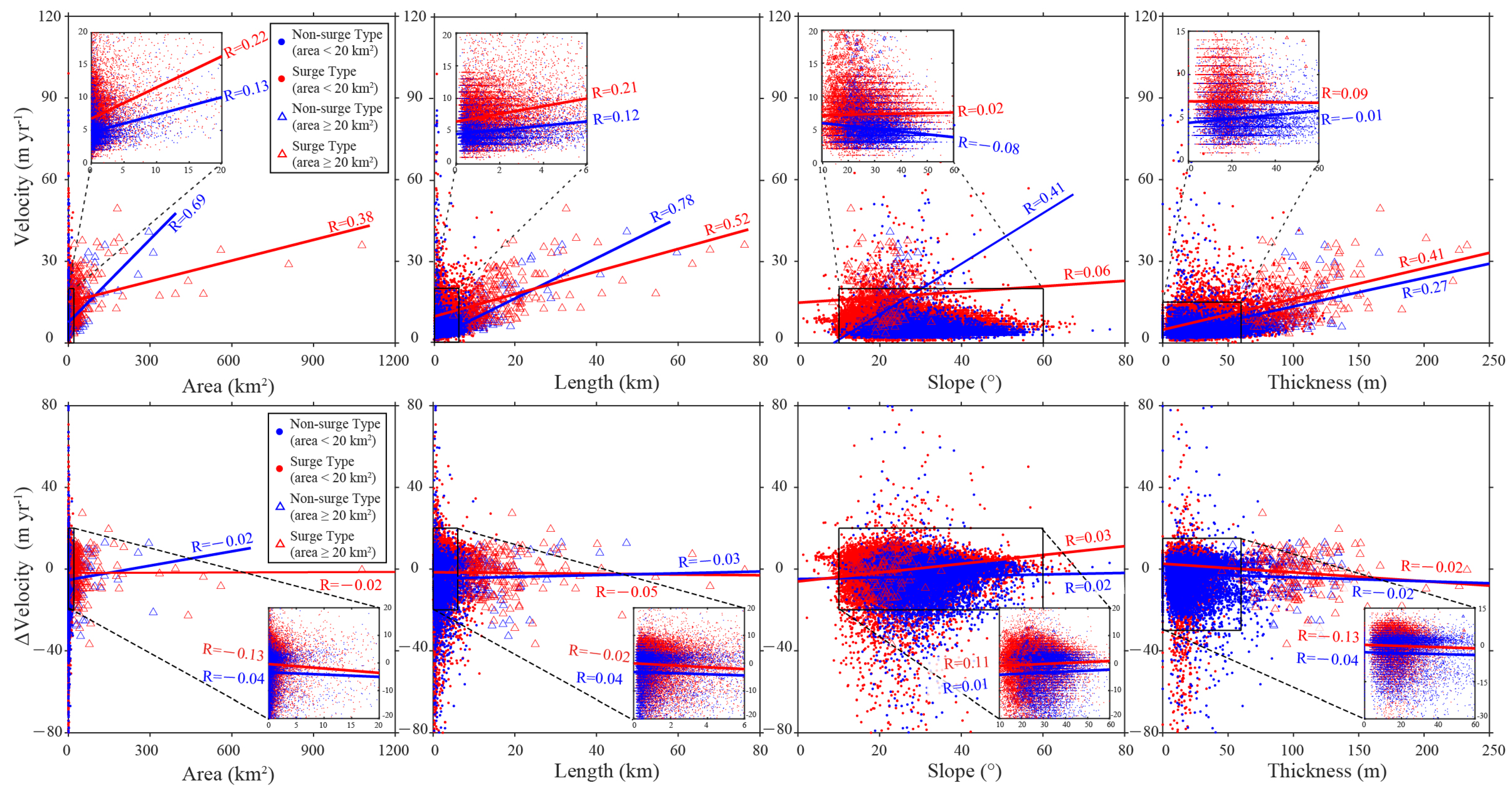
4. Results

| Number of Glaciers | Speedup | Slowdown | Stable | Speedup (m yr) | Slowdown (m yr) | Overall (m yr dec) | ||||
|---|---|---|---|---|---|---|---|---|---|---|
| Average | Maximum | Average | Maximum | This Study | [9] | |||||
| Hindu Kush | 4206 | 22.6% | 28.3% | 49.1% | 5.2 | 29.6 (RGI60-14.24088) | −11.5 | −186.0 (RGI60-14.22312) | −1.0 | −1.4 |
| Karakoram | 12,822 | 17.3% | 31.5% | 51.2% | 6.6 | 127.7 (RGI60-14.04875) | −13.7 | −256.7 (RGI60-14.03000) | −1.6 | 0.8 |
| Spiti Lahaul | 7796 | 19.6% | 18.7% | 61.7% | 6.4 | 81.5 (RGI60-14.19261) | −12.1 | −179.0 (RGI60-14.17193) | −0.4 | −4.6 |
| West Nepal | 3906 | 33.4% | 29.1% | 37.5% | 5.5 | 27.2 (RGI60-14.12426) | −9.7 | −51.4 (RGI60-15.05231) | −0.5 | −2.2 |
| East Nepal | 3563 | 56.2% | 19.6% | 24.2% | 6.3 | 55.8 (RGI60-15.09859) | −12.3 | −62.0 (RGI60-15.09861) | 0.7 | −1.8 |
| Bhutan | 1547 | 34.1% | 22.1% | 43.8% | 6.6 | 39.5 (RGI60-15.02102) | −8.5 | −61.3 (RGI60-15.01907) | 0.2 | −2.1 |
| Nyainqentanglha | 2882 | 41.3% | 21.9% | 36.8% | 6.9 | 95.9 (RGI60-15.12714) | −12.4 | −135.6 (RGI60-15.12081) | 0.2 | −6.4 |
| Total | 36,722 | 32.0% | 24.5% | 43.5% | 6.3 | 127.7 (Karakoram) | −12.3 | −256.7 (Karakoram) | −0.3 | / |
5. Discussion
5.1. Regional Patterns of Surface Velocity Changes
5.2. Linking Surface Velocity Changes with Glacier Mass Balance
6. Conclusions
Author Contributions
Funding
Data Availability Statement
Acknowledgments
Conflicts of Interest
References
- Kaser, G.; Großhauser, M.; Marzeion, B. Contribution potential of glaciers to water availability in different climate regimes. Proc. Natl. Acad. Sci. USA 2010, 107, 20223–20227. [Google Scholar] [CrossRef] [PubMed] [Green Version]
- Kääb, A.; Berthier, E.; Nuth, C.; Gardelle, J.; Arnaud, Y. Contrasting patterns of early twenty-first-century glacier mass change in the Himalayas. Nature 2012, 488, 495–498. [Google Scholar] [CrossRef] [PubMed]
- Bolch, T.; Kulkarni, A.; Kääb, A.; Huggel, C.; Paul, F.; Cogley, J.G.; Frey, H.; Kargel, J.S.; Fujita, K.; Scheel, M.; et al. The state and fate of Himalayan glaciers. Science 2012, 336, 310–314. [Google Scholar] [CrossRef] [PubMed] [Green Version]
- Yao, T.; Thompson, L.; Yang, W.; Yu, W.; Gao, Y.; Guo, X.; Yang, X.; Duan, K.; Zhao, H.; Xu, B.; et al. Different glacier status with atmospheric circulations in Tibetan Plateau and surroundings. Nat. Clim. Chang. 2012, 2, 663–667. [Google Scholar] [CrossRef]
- Kraaijenbrink, P.; Bierkens, M.; Lutz, A.; Immerzeel, W. Impact of a global temperature rise of 1.5 degrees Celsius on Asia’s glaciers. Nature 2017, 549, 257–260. [Google Scholar] [CrossRef] [PubMed]
- Ren, J.; Jing, Z.; Pu, J.; Qin, X. Glacier variations and climate change in the central Himalaya over the past few decades. Ann. Glaciol. 2006, 43, 218–222. [Google Scholar] [CrossRef] [Green Version]
- Brun, F.; Berthier, E.; Wagnon, P.; Kääb, A.; Treichler, D. A spatially resolved estimate of High Mountain Asia glacier mass balances from 2000 to 2016. Nat. Geosci. 2017, 10, 668–673. [Google Scholar] [CrossRef]
- Lutz, A.; Immerzeel, W.; Shrestha, A.; Bierkens, M. Consistent increase in High Asia’s runoff due to increasing glacier melt and precipitation. Nat. Clim. Chang. 2014, 4, 587–592. [Google Scholar] [CrossRef] [Green Version]
- Dehecq, A.; Gourmelen, N.; Gardner, A.S.; Brun, F.; Goldberg, D.; Nienow, P.W.; Berthier, E.; Vincent, C.; Wagnon, P.; Trouvé, E. Twenty-first century glacier slowdown driven by mass loss in High Mountain Asia. Nat. Geosci. 2019, 12, 22–27. [Google Scholar] [CrossRef]
- Immerzeel, W.W.; Droogers, P.; De Jong, S.; Bierkens, M. Large-scale monitoring of snow cover and runoff simulation in Himalayan river basins using remote sensing. Remote Sens. Environ. 2009, 113, 40–49. [Google Scholar] [CrossRef]
- Guo, W.; Liu, S.; Xu, J.; Wu, L.; Shangguan, D.; Yao, X.; Wei, J.; Bao, W.; Yu, P.; Liu, Q.; et al. The second Chinese glacier inventory: Data, methods and results. J. Glaciol. 2015, 61, 357–372. [Google Scholar] [CrossRef] [Green Version]
- Bookhagen, B.; Burbank, D.W. Toward a complete Himalayan hydrological budget: Spatiotemporal distribution of snowmelt and rainfall and their impact on river discharge. J. Geophys. Res. Earth Surf. 2010, 115. [Google Scholar] [CrossRef] [Green Version]
- Neckel, N.; Kropáček, J.; Bolch, T.; Hochschild, V. Glacier mass changes on the Tibetan Plateau 2003–2009 derived from ICESat laser altimetry measurements. Environ. Res. Lett. 2014, 9, 014009. [Google Scholar] [CrossRef]
- Kääb, A.; Treichler, D.; Nuth, C.; Berthier, E. Brief Communication: Contending estimates of 2003–2008 glacier mass balance over the Pamir–Karakoram–Himalaya. Cryosphere 2015, 9, 557–564. [Google Scholar] [CrossRef] [Green Version]
- Maurer, J.; Schaefer, J.; Rupper, S.; Corley, A. Acceleration of ice loss across the Himalayas over the past 40 years. Sci. Adv. 2019, 5, eaav7266. [Google Scholar] [CrossRef] [PubMed] [Green Version]
- Ragettli, S.; Bolch, T.; Pellicciotti, F. Heterogeneous glacier thinning patterns over the last 40 years in Langtang Himal, Nepal. Cryosphere 2016, 10, 2075–2097. [Google Scholar] [CrossRef] [Green Version]
- Zhou, Y.; Li, Z.; Li, J.; Zhao, R.; Ding, X. Glacier mass balance in the Qinghai–Tibet Plateau and its surroundings from the mid-1970s to 2000 based on Hexagon KH-9 and SRTM DEMs. Remote Sens. Environ. 2018, 210, 96–112. [Google Scholar] [CrossRef]
- Dehecq, A.; Gourmelen, N.; Trouvé, E. Deriving large-scale glacier velocities from a complete satellite archive: Application to the Pamir–Karakoram–Himalaya. Remote Sens. Environ. 2015, 162, 55–66. [Google Scholar] [CrossRef] [Green Version]
- Shugar, D.; Jacquemart, M.; Shean, D.; Bhushan, S.; Upadhyay, K.; Sattar, A.; Schwanghart, W.; McBride, S.; de Vries, M.V.W.; Mergili, M.; et al. A massive rock and ice avalanche caused the 2021 disaster at Chamoli, Indian Himalaya. Science 2021, 373, 300–306. [Google Scholar] [CrossRef] [PubMed]
- Muhuri, A.; Gascoin, S.; Menzel, L.; Kostadinov, T.; Harpold, A.; Sanmiguel-Vallelado, A.; Moreno, J.I.L. Performance Assessment of Optical Satellite Based Operational Snow Cover Monitoring Algorithms in Forested Landscapes. IEEE J. Sel. Top. Appl. Earth Obs. Remote Sens. 2021, 14, 7159–7178. [Google Scholar] [CrossRef]
- Kääb, A.; Winsvold, S.H.; Altena, B.; Nuth, C.; Nagler, T.; Wuite, J. Glacier remote sensing using Sentinel-2. part I: Radiometric and geometric performance, and application to ice velocity. Remote Sens. 2016, 8, 598. [Google Scholar] [CrossRef] [Green Version]
- Azam, M.F.; Ramanathan, A.; Wagnon, P.; Vincent, C.; Linda, A.; Berthier, E.; Sharma, P.; Mandal, A.; Angchuk, T.; Singh, V.; et al. Meteorological conditions, seasonal and annual mass balances of Chhota Shigri Glacier, western Himalaya, India. Ann. Glaciol. 2016, 57, 328–338. [Google Scholar] [CrossRef] [Green Version]
- Sun, Y.; Jiang, L.; Liu, L.; Sun, Y.; Wang, H. Spatial-temporal characteristics of glacier velocity in the Central Karakoram revealed with 1999–2003 Landsat-7 ETM+ Pan Images. Remote Sens. 2017, 9, 1064. [Google Scholar] [CrossRef] [Green Version]
- Fujita, K. Effect of precipitation seasonality on climatic sensitivity of glacier mass balance. Earth Planet. Sci. Lett. 2008, 276, 14–19. [Google Scholar] [CrossRef]
- Immerzeel, W.; Wanders, N.; Lutz, A.; Shea, J.; Bierkens, M. Reconciling high-altitude precipitation in the upper Indus basin with glacier mass balances and runoff. Hydrol. Earth Syst. Sci. 2015, 19, 4673–4687. [Google Scholar] [CrossRef] [Green Version]
- Dumont, M.; Gascoin, S. Optical remote sensing of snow cover. In Land Surface Remote Sensing in Continental Hydrology; Elsevier: Amsterdam, The Netherlands, 2016; pp. 115–137. [Google Scholar]
- Farr, T.G.; Rosen, P.A.; Caro, E.; Crippen, R.; Duren, R.; Hensley, S.; Kobrick, M.; Paller, M.; Rodriguez, E.; Roth, L.; et al. The shuttle radar topography mission. Rev. Geophys. 2007, 45. [Google Scholar] [CrossRef] [Green Version]
- Farinotti, D.; Huss, M.; Fürst, J.J.; Landmann, J.; Machguth, H.; Maussion, F.; Pandit, A. A consensus estimate for the ice thickness distribution of all glaciers on Earth. Nat. Geosci. 2019, 12, 168–173. [Google Scholar] [CrossRef] [Green Version]
- Leprince, S.; Barbot, S.; Ayoub, F.; Avouac, J.P. Automatic and precise orthorectification, coregistration, and subpixel correlation of satellite images, application to ground deformation measurements. Geosci. Remote Sens. IEEE Trans. 2007, 45, 1529–1558. [Google Scholar] [CrossRef] [Green Version]
- Ayoub, F.; Leprince, S.; Keene, L. Users Guide to COSI-CORR Co-Registration of Optically Sensed Images and Correlation; California Institute of Technology: Pasadena, CA, USA, 2009; p. 38. [Google Scholar]
- Hooke, R.L.; Calla, P.; Holmlund, P.; Nilsson, M.; Stroeven, A. A 3 year record of seasonal variations in surface velocity, Storglaciären, Sweden. J. Glaciol. 1989, 35, 235–247. [Google Scholar] [CrossRef] [Green Version]
- Lemos, A.; Shepherd, A.; McMillan, M.; Hogg, A.E. Seasonal variations in the flow of land-terminating glaciers in Central-West Greenland using Sentinel-1 imagery. Remote Sens. 2018, 10, 1878. [Google Scholar] [CrossRef] [Green Version]
- Kraaijenbrink, P.; Meijer, S.W.; Shea, J.M.; Pellicciotti, F.; De Jong, S.M.; Immerzeel, W.W. Seasonal surface velocities of a Himalayan glacier derived by automated correlation of unmanned aerial vehicle imagery. Ann. Glaciol. 2016, 57, 103–113. [Google Scholar] [CrossRef] [Green Version]
- Glen, J. Experiments on the deformation of ice. J. Glaciol. 1952, 2, 111–114. [Google Scholar] [CrossRef] [Green Version]
- Glen, J.W. The creep of polycrystalline ice. Proc. R. Soc. Lond. Ser. A Math. Phys. Sci. 1955, 228, 519–538. [Google Scholar]
- Weertman, J. On the sliding of glaciers. J. Glaciol. 1957, 3, 33–38. [Google Scholar] [CrossRef] [Green Version]
- Goldsby, D.; Kohlstedt, D.L. Superplastic deformation of ice: Experimental observations. J. Geophys. Res. Solid Earth 2001, 106, 11017–11030. [Google Scholar] [CrossRef]
- MacAyeal, D.R. Large-scale ice flow over a viscous basal sediment: Theory and application to ice stream B, Antarctica. J. Geophys. Res. Solid Earth 1989, 94, 4071–4087. [Google Scholar] [CrossRef]
- Bocchiola, D.; Bombelli, G.M.; Camin, F.; Ossi, P.M. Field Study of Mass Balance, and Hydrology of the West Khangri Nup Glacier (Khumbu, Everest). Water 2020, 12, 433. [Google Scholar] [CrossRef] [Green Version]
- Pelto, M.; Panday, P.; Matthews, T.; Maurer, J.; Perry, L.B. Observations of Winter Ablation on Glaciers in the Mount Everest Region in 2020–2021. Remote Sens. 2021, 13, 2692. [Google Scholar] [CrossRef]
- Wagnon, P.; Vincent, C.; Arnaud, Y.; Berthier, E.; Vuillermoz, E.; Gruber, S.; Ménégoz, M.; Gilbert, A.; Dumont, M.; Shea, J.; et al. Seasonal and annual mass balances of Mera and Pokalde glaciers (Nepal Himalaya) since 2007. Cryosphere 2013, 7, 1769–1786. [Google Scholar] [CrossRef] [Green Version]
- Wagnon, P.; Brun, F.; Khadka, A.; Berthier, E.; Shrestha, D.; Vincent, C.; Arnaud, Y.; Six, D.; Dehecq, A.; Ménégoz, M.; et al. Reanalysing the 2007–19 glaciological mass-balance series of Mera Glacier, Nepal, Central Himalaya, using geodetic mass balance. J. Glaciol. 2021, 67, 117–125. [Google Scholar] [CrossRef]

Publisher’s Note: MDPI stays neutral with regard to jurisdictional claims in published maps and institutional affiliations. |
© 2021 by the authors. Licensee MDPI, Basel, Switzerland. This article is an open access article distributed under the terms and conditions of the Creative Commons Attribution (CC BY) license (https://creativecommons.org/licenses/by/4.0/).
Share and Cite
Zhou, Y.; Chen, J.; Cheng, X. Glacier Velocity Changes in the Himalayas in Relation to Ice Mass Balance. Remote Sens. 2021, 13, 3825. https://doi.org/10.3390/rs13193825
Zhou Y, Chen J, Cheng X. Glacier Velocity Changes in the Himalayas in Relation to Ice Mass Balance. Remote Sensing. 2021; 13(19):3825. https://doi.org/10.3390/rs13193825
Chicago/Turabian StyleZhou, Yu, Jianlong Chen, and Xiao Cheng. 2021. "Glacier Velocity Changes in the Himalayas in Relation to Ice Mass Balance" Remote Sensing 13, no. 19: 3825. https://doi.org/10.3390/rs13193825
APA StyleZhou, Y., Chen, J., & Cheng, X. (2021). Glacier Velocity Changes in the Himalayas in Relation to Ice Mass Balance. Remote Sensing, 13(19), 3825. https://doi.org/10.3390/rs13193825