Abstract
A current hindrance to the scientific use of available bathymetric lidar point clouds is the frequent lack of accurate and thorough segmentation of seafloor points. Furthermore, scientific end-users typically lack access to waveforms, trajectories, and other upstream data, and also do not have the time or expertise to perform extensive manual point cloud editing. To address these needs, this study seeks to develop and test a novel clustering approach to seafloor segmentation that solely uses georeferenced point clouds. The proposed approach does not make any assumptions regarding the statistical distribution of points in the input point cloud. Instead, the approach organizes the point cloud into an inverse histogram and finds a gap that best separates the seafloor using the proposed peak-detection method. The proposed approach is evaluated with datasets acquired in Florida with a Riegl VQ-880-G bathymetric LiDAR system. The parameters are optimized through a sensitivity analysis with a point-wise comparison between the extracted seafloor and ground truth. With optimized parameters, the proposed approach achieved F1-scores of 98.14–98.77%, which outperforms three popular existing methods. Further, we compared seafloor points with Reson 8125 MBES hydrographic survey data. The results indicate that seafloor points were detected successfully with vertical errors of −0.190 ± 0.132 m and −0.185 ± 0.119 m (μ ± σ) for two test datasets.
1. Introduction
The volume of bathymetric lidar point clouds available to coastal scientists, engineers, and coastal zone managers is increasing rapidly. Many datasets are available on portals, such as the National Oceanic and Atmospheric Administration (NOAA) Digital Coast [1], state GIS clearinghouses, and others. However, a current impediment to effective use of these bathymetric lidar point clouds is that many lack accurate point classification (specifically, the segmentation of points into water surface, water column noise, and seafloor points) [2,3]. Accurate segmentation of seafloor (or lakebed or riverbed, depending on the area) points, often referred to as “bathymetric bottom”, is critically important to a number of processing and analysis tasks, including hydrodynamic modeling, benthic habitat mapping, and sediment transport studies [4,5,6,7].
There are a number of reasons why a given bathymetric lidar point cloud may lack accurate point classification. In a few cases, point classification may never have been performed. As just one example, while many studies have documented the presence of bathymetry in geolocated photon returns from NASA’s ICESat-2 ATLAS [8,9,10], the processing algorithms used to generate the point datasets make no attempt to assign bathymetric point classes. More often (and especially in the case of airborne lidar) point classification has been performed, but sometimes only through rough, automated routines, which can result in a number of errors of both omission and commission in segmenting bathymetric bottom points. Depending on the processing settings used by the data provider, the bathymetric bottom will often be under-segmented, meaning that actual bathymetric returns end up in a noise class (see Figure 1). In turn, this can lead to sparse bathymetry and poor or incomplete seafloor models. In other cases, depending on the processing stream prior to a bathymetric lidar point cloud being made available to an end-user, the point class assignments may simply have been lost (inadvertently removed) at some point in the processing. Regardless of the cause, it is not at all uncommon for an end user to receive a bathymetric lidar point cloud with no point classes assigned (just an undifferentiated conglomeration of seafloor, water surface, and water column points), or with rough point classification that may not meet scientific needs (Figure 1).
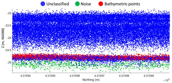
Figure 1.
Bathymetric point cloud data acquired in Marco island located in Miami, Florida, USA [11], indicating possible under-segmentation of bathymetric bottom. Note the presence of a gap between the lowest water column points and the bathymetric bottom, which is leveraged in this work.
For scientific end users who need to perform their own bathymetric bottom point segmentation on a lidar point cloud, there are numerous challenges. First, end-users typically do not have access to the lidar waveforms, trajectories, or other “upstream” data that would be available to the data acquisition organization or others in earlier stages of the processing stream. Second, such users generally do not have access to specialized software for bathymetric lidar processing or expertise in such processing. And, while there are a number of commercial processing software tools that provide functionality for manual point classification (often by presenting to the user profile views or vertical slices of points, such that they can manually draw boxes around different point classes), this is a very laborious process that would take time away from scientific analysis. For these reasons, there is a current need for algorithms and workflows for straightforward, automated segmentation of bathymetric bottom points in lidar point clouds. Desirable characteristics of such algorithms are: (1) efficiency; (2) ease of implementation; (3) avoidance of the need to have waveforms, trajectories, or other ancillary data; and (4) avoidance of any assumptions regarding point distributions (for example, the requirement that points be normally distributed). Some existing methods [2,3,12,13,14] that use machine learning algorithms have demonstrated good results in seafloor segmentation, but do not meet the needs outlined above, due to necessitating a large number of input variables (in some cases, including full waveforms or waveform-derived features) and data labeling, which would not be available to many scientific users of the data.
Fortunately, a salient characteristic of point clouds from conventional airborne, linear-mode bathymetric lidar systems is the presence of a vertical gap between the lowest water column points and the bathymetric bottom [15]. This gap is clearly discernable in Figure 1. As explained in [15], the general cause of this gap is the range discrimination threshold, or the size of the “dead zone” following each detected return before another return can be resolved. In theory, the range resolution is given by , where υ is the velocity of the laser light in the applicable medium (air or water) and is the transmit pulse width [16]. In practice, the actual range resolution can be longer or shorter, depending on the ranging hardware or software used [17,18]. For the Riegl VQ-880-G used to acquire the Florida datasets used in this study, the transmit pulse width is 1.3 ns [19], such that the expected width of the water column-seafloor gap is ~15 cm.
The existence of the water column-seafloor gap suggests the feasibility of a straightforward approach to seafloor point segmentation that meets all of the desired characteristics listed above and can easily be applied by scientific end-users to existing bathymetric lidar point clouds lacking accurate seafloor point segmentation. The approach developed and tested in this work does not assume any particular statistical distribution of points. Instead, it finds a gap between the seafloor and non-seafloor (e.g., water surface and water column) points by investigating the distribution of the points in the z-direction. It is important to note that the input for the proposed approach is solely geometric information (i.e., x, y, and z coordinates) of the point cloud; it does not require waveforms, intensity values, aircraft trajectories, or other data that may not be available to end-users.
2. Methods
We propose a simple, effective approach to seafloor segmentation from the bathymetric lidar point cloud using an inverse histogram with the proposed peak detection method. Note that all of the symbols used in the proposed algorithm are listed in Table A1. Prior to organizing the point cloud into a histogram, it is desirable to discretize the point cloud into smaller groups of points in x-y dimension to reduce the z-variations of the seafloor over a localized area, and thus increasing the gap between the seafloor and non-seafloor points. For this purpose, the original input point cloud is organized into a regularly spaced 2D grid cell structure using the x and y values. This step contains an inherent tradeoff in selecting the grid cell size, . A smaller value of yields a more distinguishable z value distribution between the seafloor and other points but increases the computational load and over-segmentation. The selection of the input grid-cell size will be further discussed in Section 3.
After organizing the point cloud into the grid cells, the proposed seafloor segmentation is performed separately for the points of each grid cell. The points in a grid cell are sorted in descending order of z-value to compute a histogram. The points may include some outliers due primarily to birds or diffused noisy points, which can incur the largest gap above the sea surface or below the seafloor. Since the proposed algorithm assumes that the largest gap exists between the seafloor and non-seafloor points, it is desirable to discard the outliers from the histogram-based clustering. To that end, the points within the lower or upper bounds are identified with a pre-specified value, (%), as shown in Figure 2, which limits the algorithm to find a gap only between the lower and upper bounds, such that the outliers within the bounds are excluded from the histogram clustering. If is too small, the lower or upper bounds may not be large enough to include all outliers within the bounds, whereas too large of a value could lead to the largest gap within either the lower or upper bound. The selection of the input bound rate will be discussed in Section 3. In addition, was used to remove the small bins that fall within the bottom percentile of the bin containing the largest number of points in the histogram. Figure 2 shows an example of the histogram created using a cell size of 10 m, where the bin size () and the bound rate were determined to be 0.05 m and 2.5%, respectively.
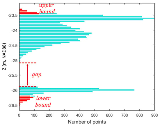
Figure 2.
Histogram representing the number of points of a grid cell. The gap between the seafloor and non-seafloor and the bins within the lower and upper bounds are highlighted in red.
Figure 2 also highlights the gap that best divides the seafloor and non-seafloor. In order to identify the gap, we propose a peak detection using an inverse histogram. Figure 3 provides an example of the inverse histogram generated after removing the points within the upper and lower bounds. The algorithm visits each bin (, where is the total number of bins) and evaluates the count of with its two neighbors ( and ). If the count of is greater than that of , is stored into a candidate peak () and evaluated further with . If the count of is less than that of , the algorithm deletes ; otherwise, if the count of is equal to , is retained. Finally, if the count of is greater than , is stored as a detected peak. The algorithm iterates to grow as long as the count of is equal to , allowing a single peak to contain multiple bins. Algorithm 1 includes the details of the proposed peak detection method. In Figure 3, the purple bins represent the three peaks (, , and ) detected using the proposed peak detection method.
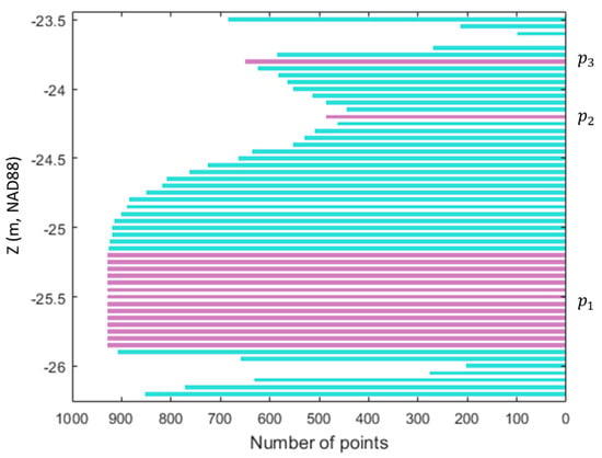
Figure 3.
Examples of detected peaks (
, , and ) in the inverse histogram.
| Algorithm 1. Peak Detection Method | |
| 1 | Input: histogram bins (), Output: peaks () |
| 2 | Set |
| 3 | Set |
| 4 | While , where is the total number of bins |
| 5 | If the count of > |
| 6 | While true |
| 7 | Add current to candidate peak () |
| 8 | If |
| 9 | is deleted |
| 10 | Break; |
| 11 | Else if the count of |
| 12 | Add current to detected peak () |
| 13 | is deleted |
| 14 | Set |
| 15 | Break |
| 16 | Set |
| 17 | End While |
| 18 | Set |
| 19 | End While |
| 20 | Return , where is the total number of detected peaks |
After detecting the peaks, the one that best divides the seafloor and non-seafloor is identified. For this purpose, the total number of points for each peak is counted from the inverse histogram to select the peak with the largest number of points. This gives a larger weight to the peak with a greater number of empty bins in the original histogram, enabling one to maximize the gap between the seafloor and non-seafloor. For example, among the detected peaks (, , and ) in Figure 3, the algorithm selects with the largest number of points in the inverse histogram as the best peak which corresponds to the gap in the original histogram in Figure 2.
Subsequently, the median of the z-values of the bins contained in the selected best peak is used as a threshold to divide the original histogram into the lower and upper segments, respectively. Figure 4 shows that the original histogram is divided into two segments, where the one with the lower mean z values is chosen as the seafloor. Note that if no peak is found in the inverse histogram (i.e., there is only one peak in the original histogram), there is a good chance that the cell does not contain the points returned from the seafloor. Accordingly, in this case, the entire points in the cell are segmented into non-seafloor. Finally, using the threshold, the original point cloud within the cell is segmented into the seafloor and non-seafloor as shown in Figure 5. This process is repeated iteratively until all of the cells are tested and segmented.
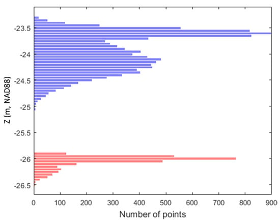
Figure 4.
Histogram divided into upper and lower segments. The lower segment is determined to be the seafloor.
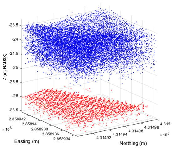
Figure 5.
Segmented seafloor (red) and non-seafloor (blue) points.
3. Results
The proposed approach was tested on airborne lidar bathymetry (ALB) datasets acquired offshore of Marco Island and Virginia Key, Florida, using the NOAA National Geodetic Survey (NGS) Remote Sensing Division’s Riegl VQ-880-G system (532 nm wavelength). Marco Island is a barrier island in the Gulf of Mexico in southwest Florida, with offshore areas containing primarily sandy substrate and some seagrass beds [20]. Virginia Key in Miami, Florida, is a barrier island in Biscayne Bay, and the location of NOAA’s Atlantic Oceanographic and Meteorological Laboratory (AOML). Surrounding substrate types include sand, mud, coarse shell, and rubble, with cover including seagrass [21]. The Marco Island datasets were chosen to evaluate the algorithm on the near-shore area, while Virginia Key datasets were chosen for the comparison with the multibeam echosounder (MBES) hydrographic survey data. Figure 6 and Table 1 shows test sites and the details of ALB datasets relevant to the experiment. Note that the Marco Island datasets were provided in NAD83(2011) ellipsoid height, and the Virginia Key datasets were provided in NAVD88 orthometric height at the time of file downloading. In Figure 6b, Virginia Key datasets were transformed to NAD88 for consistency. Also, the ESRI ArcGIS satellite background images and the ALB data in Figure 6a were obtained at different tidal levels. Therefore, the digital elevation model was added to show the exact shoreline when the lidar data was obtained. The reported accuracy of the ALB data is ±0.15 m () vertical and ±1.0 m () horizontal [11,22]. Before the experiments, the outliers (e.g., returns from birds, atmospheric particles, and/or system noise) in the datasets were reduced using a statistical outlier removal filter in the point cloud processing software CloudCompare v 2.11.3. The algorithm computes the average distance and standard deviation of each point to its neighbors and then removes the outlier points using the sigma rules [23]. In this study, we empirically set the number of neighbors to 10 and the standard deviation multiplier threshold to 3 (i.e., 3 sigma), considering the point density and noise level of the datasets. The Marco Island datasets # 1 and 2 were used to evaluate the developed approach’s sensitivity to the three input parameters (, , and ) and the datasets # 3 to 6 were used to evaluate the developed approach’s robustness against other three existing clustering methods (Expectation and Maximization, Otsu, and k-means algorithms). For ground-truthing, the seafloor points were labeled manually using the classification features in Maptek I-Site Studio 7.0. For a robust comparison, we evaluated the methods under challenging testing conditions with shallow areas of water depth < 5–7 m.
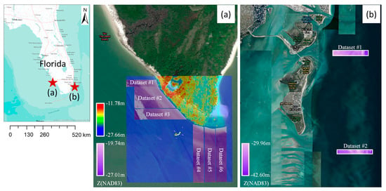
Figure 6.
Test sites: (a) Marco Island and (b) Virginia Key located in Miami, Florida, USA.

Table 1.
Data set and acquisition parameters. Note that the point densities refer to all returns (e.g., seafloor, water column, and sea surface) and encompass overlapping flight lines. LMSL refers to the local mean sea level tidal datum.
The Virginia Key datasets were used to compare the seafloor point cloud segmented by the proposed approach with the MBES data acquired by NOAA in 2009 using a Reson 8125 MBES. According to the metadata, the reported accuracy of the MBES data satisfied the IHO Order 1 total uncertainty standards (95% confidence level) [24]. For direct comparison, a vertical datum transformation using VDatum v4.1.1 from mean lower low water (MLLW) to NAVD88 was performed. Note that due to the eight-year temporal offset between the MBES and lidar data acquisition, we purposefully selected comparison sites far enough offshore to be less impacted by nearshore processes (e.g., breaking waves and nearshore currents) and shifting sandbars in the Virginia Key dataset.
3.1. Sensitivity Analysis
The optimal parameters of the proposed approach were determined through a sensitivity analysis of the test variables listed in Table 2 using Marco Island datasets # 1 and #2. The experiments were conducted in a MATLAB implementation running on a computer with an Intel® Core™ i7-4712MQ CPU (2.3 GHz, 16 GB RAM). To evaluate the performance, a pointwise comparison was performed between the segmented seafloor and the ground truth in terms of precision, recall, and F1 score calculations. We investigated all the combinations of three parameters (, , and ) with five to six test variables, which results in a total of 5 × 5 × 6 = 150 combinations.

Table 2.
Test variables for sensitivity analysis.
The range of the test variables had been determined from the preliminary experimentation. The cell size, , plays a pivotal role in the overall behavior of seafloor segmentation. The smaller the value of , the more details of the seafloor can be segmented. However, the smaller leads to a high computational load and over-segmentation for the cells containing no points returned from the seafloor. We found that the cell sizes of less than 2.0 m led to many cells containing no seafloor points, and therefore, the test variables were set between 2.0 and 10.0 m in 2.0 m increments. The test variables for were set between 0.02 and 0.10 m in 0.02 m increments. The larger the value, the fewer the bins that are evaluated, enabling the computational load to be reduced. However, too large values may not preserve the variability in the distribution, thus leading to a failure in the peak detection. Finally, the test variables for were set between 0 and 5% in 1% increments. Too small of a value may increase the chance of finding an incorrect gap, due to remaining outliers, whereas too large of a value may increase the chance of having both the seafloor and non-seafloor points in either an upper or lower bound. Note that the minimum value was set to 0% to demonstrate the usefulness of compared with its absence results.
Table 3 and Table 4 list the top and bottom 10 combinations of the seafloor segmentation parameters in the descending and ascending order of F1 scores, respectively. The efficiency in the tables does not include time elapsed for loading the lidar data. In Table 3, the proposed approach achieved the best F1-score of 98.85% with the optimized parameter set (: 10 m, : 0.02 m, and : 1%). The cell sizes of both the top and bottom 10 combinations tend to have large values of 10 m. This is due to the fact that, although large cell sizes help prevent over-segmentation with small bin sizes, large bin sizes can lead large cell sizes to more over-segmentation due to the low variability in the distribution. Table 3 and Table 4 also show that larger cell sizes are desirable for more efficient processing. The bin sizes of the top 10 combinations in Table 3 have small values ranging from 0.02 to 0.04 m, whereas all the bottom 10 combinations in Table 4 have the same largest value of 0.10 m. Compared with the cell size, efficiency is less sensitive to the bin size (for example, 186 thousand points/s with : 8 m, : 0.02 m, : 3% in Table 3 and 249 thousand points/s with : 8 m, : 0.10 m, : 3% in Table 4), so it is recommended to use small bin sizes. Finally, the bound of the top 10 combinations in Table 3 tends to have small values between 1 and 2%, whereas the bottom 10 combinations in Table 4 have large values between 3 and 5%. As with the bin size, the efficiency is less sensitive to bound (for example, 301 thousand points/s with : 10 m, : 0.10 m, : 2% and 326 thousand points/s with : 10 m, : 0.10 m, : 5% in Table 4), so the use of small values is desirable.

Table 3.
Top 10 combinations of parameters for the seafloor segmentation with Marco dataset # 1 and 2.

Table 4.
Bottom 10 combinations of parameters for the seafloor segmentation with Marco dataset # 1 and 2.
3.2. Comparison with Other Methods
With the optimized parameters (λ: 10 m, β: 0.02 m, and ω: 1%) determined from the sensitivity analysis, we further investigated the feasibility of the proposed approach with the Marco Island datasets # 3 to 6. In Table 5, the performance of the proposed approach is compared with three popular clustering methods, Expectation Maximization for Gaussian Mixture Models (EM-GMM) [25,26], Otsu [27], and k-means [28]. Otsu’s method has been widely adopted in image binarization. The algorithm organizes the pixel values into a histogram. For every bin (1, 2, 3, …, m = total number of bins of the histogram), the histogram is divided into a left histogram (1, …, n) and a right histogram (n + 1, …, m) to calculate their variances, respectively. Finally, the algorithm returns n that results in two histograms with minimum intra-class variance. Otsu’s method is known to work well on the clustering of a bi-modal distribution [29]. k-means algorithm first reassigns points to their nearest cluster centroid and then recalculates the cluster centroids. This process is repeated to minimize the sum of point-to-centroid distances of all k clusters until a new iteration does not reassign any points. k-means clustering can be improved by selecting the initial seeds [30]. In this study, the bottom and top points in the z-axis were selected for the seeds of the seafloor and non-seafloor, respectively. EM-GMM is similar to k-means in the sense that it iteratively refines the clusters through the two steps: expectation and maximization. However, unlike the k-means algorithm that uses the Euclidean distance, EM-GMM is predicated on the underlying distributions being Gaussian. The expectation step estimates the latent value (i.e., the probability of belonging to a certain cluster) for each point, and the maximization step uses maximum likelihood to optimize the parameters of the Gaussian distributions [25,26]. Like the proposed approach, the three existing methods were performed separately for the points of each grid cell with a cell size of 10 m.

Table 5.
Performance comparison of four segmentation methods (Otsu, EM-GMM, k-means, and the proposed) using Marco datasets # 3, 4, 5, and 6.
Overall, the experimental results in Figure 7 and Table 5 demonstrate that the proposed approach outperforms the other methods in terms of the F1-scores while maintaining high efficiency. The poor F1-scores (81.77–95.29% in Table 5) achieved with Otsu and EM-GMM methods are primarily due to the fact that they assume a bi-modal distribution for clustering, which does not hold true for many cases as can be seen in Figure 8a due to the points returned from the water column. On the other hand, k-means, which uses spatial extent to split the data, achieved F1-scores of 92.15–98.16%. While this performance exceeded that of the Otsu and EM-GMM methods, it still did not match that of our approach (98.14–98.77%) since k-means tends to not converge to solution especially for imbalanced datasets as can be seen in Figure 8b. In addition, all the approaches including the proposed one are susceptible to over-segmentation for the cells with no seafloor points (Figure 8c) or with mixed bins that cannot be segmented using a single threshold (Figure 8d), which will be studied in future works.
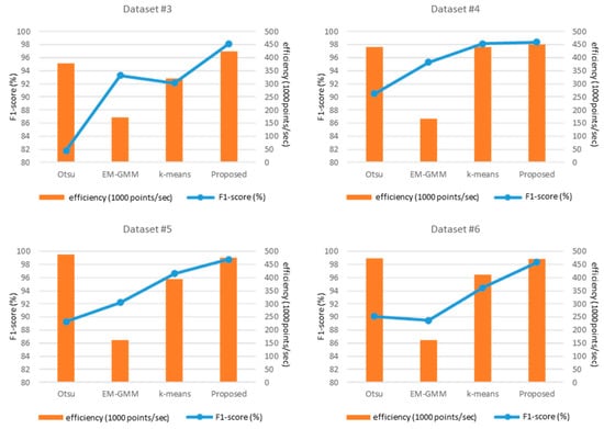
Figure 7.
Performance comparison of four segmentation methods (Otsu, EM-GMM, k-means, and the proposed) using Marco datasets # 3, 4, 5, and 6.
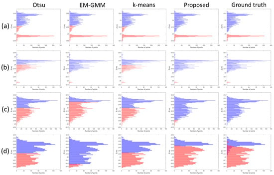
Figure 8.
Example histograms showing segmented seafloor (red) and non-seafloor (blue) segments of Marco datasets with cell number: (a) 4–149; (b) 3–6; (c) 3–52; and (d) 5–148. All the example datasets are in NAD88 height.
3.3. Comparison with MBES Hydrographic Data
Finally, with the optimized parameters, the Virginia Key datasets # 1 and # 2 were segmented and compared with the MBES hydrographic survey data collected over the same area. The MBES datasets were provided online in a raster format with a cell size of 1 m [31]. The seafloor points segmented using the proposed approach were projected onto the MBES data to calculate difference maps in the z-direction using the CloudCompare v 2.11.3. Since NOAA only provides the MBES datasets in the grid (rasterized) format for the study site (Virginia Key), vertical accuracy was assessed by comparing the elevation of the represented surface of the MBES dataset to elevations of the segmented ALB points at their horizontal (x and y) coordinates [32].
The results indicate that seafloor points were detected successfully with errors calculated to be −0.190 ± 0.132 m and −0.185 ± 0.119 m (μ ± σ) for the Virginia Key datasets # 1 and # 2, respectively. It is worth noting that the vertical datum transformation uncertainty of ~7 cm [19,33] may have contributed to the computed errors. Figure 9a shows the MBES dataset used for the comparison with the Virginia dataset # 1, Figure 9b shows the difference map between the segmented seafloor and the MBES dataset, and Figure 9c shows the histogram of the pixel values of the difference map, respectively. In Figure 9c, it can be seen that the pixel values are distributed randomly over the test site.
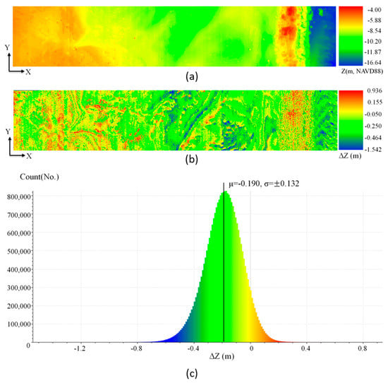
Figure 9.
Error distribution in the z-direction (z) of Virginia dataset # 1; (a) MBES data of Virginia test site # 1 (b) The difference map of z (c) Frequency histogram of z ( < z < ).
4. Discussion
Although the proposed approach was proven to be an effective means of seafloor segmentation, there are some issues requiring further investigation. As with other clustering methods, the proposed approach is set to split two clusters (i.e., seafloor and non-seafloor), thereby leading to over-segmentation in some areas containing no points returned from the seafloor. This could possibly be addressed by using other attributes in the bathymetric point cloud data, such as intensity and return number, to identify and remove the over-segmented clusters. Another issue is the mixed bins that cannot be split using a single threshold. There is an inherent tradeoff in tackling both challenges since a large cell size is required to reduce the cells with no seafloor points while a small cell size is conducive to the mixed bins to ensure more distinguishable z variation between the seafloor and non-seafloor. The authors are currently investigating the integration of a dynamic cell sizing approach that detects those areas with no seafloor points and with mixed bins and applies different cell sizes to improve the segmentation. Moreover, the proposed approach can fail if the bathymetric lidar system has a very small transmit pulse width or small receiver “dead zone”, since this will have the tendency to improve the range resolution (decrease the distance between detected returns) and, hence, decrease the width of the gap that we utilize for seafloor segmentation. While this was not an issue with the datasets in this study, the ability to handle smaller gap widths is a necessary enhancement for the wider use of the proposes approach. For example, integration of intensity values into the z values may enable the increased gap size, and this will be investigated in upcoming research.
Further, we visually inspected a number of subsets of the input point clouds along with the algorithm output, as a means of qualitative assessment and, in particular, to gain insight any possible incorrect seafloor segmentation. A key finding from this analysis was that in the few cases in which the algorithm did not detect the seafloor, the clear cause was the lack of a distinct gap between the lowest water column (volume backscatter) points and the bathymetric bottom. This makes sense, as the algorithm is predicated on the existence of this gap. This leads to the question of when the expected gap would not exist. From visual inspection of the point clouds, it was determined that there are two situations in which the expected gap is not present: (1) there is no detectable seafloor in the point cloud, which could be due to the water being deeper than the lidar extinction depth or the bottom return signal dropping below the detection threshold due to low-reflectance substrates, slope, or other seafloor characteristics [34]; or (2) there are (barely) detectable seafloor returns, but they are simply too sparse to yield a bottom return peak in the histograms. Both of these scenarios are cases in which the algorithm could not be expected to detect the seafloor, thereby forcing the algorithm to over-segment seafloor from the sea surface or column. Figure 10 shows an example of the seafloor points segmented from the Virginia Key area, containing some over-segmented points (highlighted in red) due to the missing seafloor returns. Note that Figure 10 is not the Virginia Key datasets used for the comparison but obtained from another dataset to show the over-segmentation issue. Future work could investigate the ability to utilize intensity data (beyond just the point cloud 3D spatial coordinates) to reduce the over-segmentation. Another approach to densifying seafloor returns, which involves interpolation of missing points with a priori information, will be investigated in future work. It is also worth investigating the ability to constrain the seafloor segmentation algorithm using estimates of maximum achievable depth, which, in turn, may be estimated from knowledge of diffuse attenuation coefficient of downwelling irradiance, Kd, and system and environmental parameters.
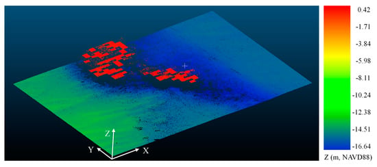
Figure 10.
An example of the seafloor points segmented from the Virginia Key area, representing an over-segmentation issue due to the missing seafloor returns.
5. Conclusions
In this study, we proposed and tested a novel clustering approach to seafloor segmentation using bathymetric lidar data. The approach uses only the geometric information of point cloud data and avoids any assumptions regarding statistical distributions of points. The approach was evaluated with datasets acquired by a Riegl VQ-880-G bathymetric lidar system. The experimental results obtained from comparisons against existing approaches demonstrated the robustness of the proposed approach in shallow areas with high F1-scores ranging from 98.14 to 98.77% while maintaining high efficiency from 0.42 to 0.47 million points/s. The output of the proposed approach was also compared against Reson 8125 MBES hydrographic survey data, and the results showed that the seafloor point cloud was segmented successfully with vertical errors of −0.190 ± 0.132 m and −0.185 ± 0.119 m (μ ± σ) for both test sites. Future work will consider expanding the current workflow to classify the segmented seafloor points into specific objects, such as coral reef, rock, sand, and noise. Further, it would be valuable to test the approach on bathymetric point clouds generated from other sources, such as structure from motion (SfM) photogrammetric workflows.
Author Contributions
Conceptualization, J.J. and J.L.; methodology, J.J.; software, J.J.; validation, J.J. and J.L.; formal analysis, J.J. and J.L.; investigation, J.J. and J.L.; resources, J.J. and J.L.; data curation, J.L.; writing—original draft preparation, J.J., J.L. and C.E.P.; writing—review and editing, C.E.P.; review of related works, C.E.P.; visualization, J.J. and J.L.; supervision, J.L.; project administration, J.L.; funding acquisition, C.E.P. and J.L. All authors have read and agreed to the published version of the manuscript.
Funding
This research was supported by Basic Science Research Program through the National Research Foundation of Korea(NRF) funded by the Ministry of Education (No. 2021R1I1A3059263) and Oregon State University internal research funds.
Institutional Review Board Statement
Not applicable.
Informed Consent Statement
Not applicable.
Data Availability Statement
The ALB datasets used for this study are available at the following web links: https://www.fisheries.noaa.gov/inport/item/48178 (accessed on 21 March 2021) and https://www.fisheries.noaa.gov/inport/item/48180 (accessed on 8 January 2021). The MBES datasets are available at the following web link: NOAA National Center for Environmental Information Bathymetric attributed grid (BAG) data H11898 Available online: https://www.ngdc.noaa.gov/nos/H10001-H12000/H11898.html (accessed on 12 June 2020).
Conflicts of Interest
The authors declare no conflict of interest. The funders had no role in the design of the study; in the collection, analyses, or interpretation of data; in the writing of the manuscript; or in the decision to publish the results.
Appendix A

Table A1.
Symbols used in the proposed algorithm.
Table A1.
Symbols used in the proposed algorithm.
| Symbol | Definition |
|---|---|
| Grid cell size (m) | |
| Upper and lower bounds in algorithm (%) | |
| Number of histogram bins | |
| Histogram bin | |
| ith detected peak | |
| c | Candidate peak |
References
- Davidson, M.A.; Miglarese, A.H. Digital coast and the national map: A seamless coorperative. Photogramm. Eng. Remote Sens. 2003, 69, 1127–1131. [Google Scholar] [CrossRef]
- Lowell, K.; Calder, B.; Lyons, A. Measuring shallow-water bathymetric signal strength in lidar point attribute data using machine learning. Int. J. Geogr. Inf. Sci. 2020, 35, 1–19. [Google Scholar]
- Lowell, K.; Calder, B. Assessing Marginal Shallow-Water Bathymetric Information Content of Lidar Sounding Attribute Data and Derived Seafloor Geomorphometry. Remote Sens. 2021, 13, 1604. [Google Scholar] [CrossRef]
- Irish, J.L.; White, T.E. Coastal engineering applications of high-resolution lidar bathymetry. Coast. Eng. 1998, 35, 47–71. [Google Scholar] [CrossRef]
- Wedding, L.M.; Friedlander, A.M.; McGranaghan, M.; Yost, R.S.; Monaco, M.E. Using bathymetric lidar to define nearshore benthic habitat complexity: Implications for management of reef fish assemblages in Hawaii. Remote Sens. Environ. 2008, 112, 4159–4165. [Google Scholar] [CrossRef]
- Chust, G.; Grande, M.; Galparsoro, I.; Uriarte, A.; Borja, Á. Capabilities of the bathymetric Hawk Eye LiDAR for coastal habitat mapping: A case study within a Basque estuary. Estuar. Coast. Shelf Sci. 2010, 89, 200–213. [Google Scholar] [CrossRef]
- Kumpumäki, T.; Ruusuvuori, P.; Kangasniemi, V.; Lipping, T. Data-driven approach to benthic Cover type classification using bathymetric LiDAR waveform analysis. Remote Sens. 2015, 7, 13390–13409. [Google Scholar] [CrossRef] [Green Version]
- Parrish, C.E.; Magruder, L.A.; Neuenschwander, A.L.; Forfinski-Sarkozi, N.; Alonzo, M.; Jasinski, M. Validation of ICESat-2 ATLAS bathymetry and analysis of ATLAS’s bathymetric mapping performance. Remote Sens. 2019, 11, 1634. [Google Scholar] [CrossRef] [Green Version]
- Albright, A.; Glennie, C. Nearshore Bathymetry From Fusion of Sentinel-2 and ICESat-2 Observations. IEEE Geosci. Remote Sens. Lett. 2020, 18, 900–904. [Google Scholar] [CrossRef]
- Thomas, N.; Pertiwi, A.P.; Traganos, D.; Lagomasino, D.; Poursanidis, D.; Moreno, S.; Fatoyinbo, L. Space-Borne Cloud-Native Satellite-Derived Bathymetry (SDB) Models Using ICESat-2 And Sentinel-2. Geophys. Res. Lett. 2021, 48, e2020GL092170. [Google Scholar] [CrossRef]
- NOAA National Geodetic Survey. 2016 NOAA NGS Topobathy Lidar: Marco Island (FL). Available online: https://www.fisheries.noaa.gov/inport/item/48178 (accessed on 21 March 2021).
- Sun, Y.-D.; Shyue, S.-W. A hybrid seabed classification method using airborne laser bathymetric data. J. Mar. Sci. Technol. 2017, 25, 12. [Google Scholar]
- Kogut, T.; Slowik, A. Classification of Airborne Laser Bathymetry Data Using Artificial Neural Networks. IEEE J. Sel. Top. Appl. Earth Obs. Remote Sens. 2021, 14, 1959–1966. [Google Scholar] [CrossRef]
- Eren, F.; Pe’eri, S.; Rzhanov, Y.; Ward, L. Bottom characterization by using airborne lidar bathymetry (ALB) waveform features obtained from bottom return residual analysis. Remote Sens. Environ. 2018, 206, 260–274. [Google Scholar] [CrossRef]
- Mandlburger, G.; Jutzi, B. On the feasibility of water surface mapping with single photon lidar. ISPRS Int. J. Geo-Inf. 2019, 8, 188. [Google Scholar] [CrossRef] [Green Version]
- Wehr, A. LiDAR Systems and Calibration, Topographic Laser Ranging and Scanning: Principles and Processing; Shan, J., Toth, C.K., Eds.; CRC Press, Taylor and Francis Group: Boca Raton, FL, USA, 2009. [Google Scholar]
- Jutzi, B.; Stilla, U. Range determination with waveform recording laser systems using a Wiener Filter. ISPRS J. Photogramm. Remote Sens. 2006, 61, 95–107. [Google Scholar] [CrossRef]
- Parrish, C.E.; Jeong, I.; Nowak, R.D.; Smith, R.B. Empirical comparison of full-waveform lidar algorithms. Photogramm. Eng. Remote Sens. 2011, 77, 825–838. [Google Scholar] [CrossRef]
- Philpot, W. Airborne Laser Hydrography II. Available online: https://ecommons.cornell.edu/handle/1813/66666 (accessed on 24 July 2021).
- Weinstein, M.P.; Heck, K.L. Ichthyofauna of seagrass meadows along the Caribbean coast of Panama and in the Gulf of Mexico: Composition, structure and community ecology. Mar. Biol. 1979, 50, 97–107. [Google Scholar] [CrossRef]
- Jarossy, S.M. An Evaluation of the Seagrass Habitat in North Biscayne Bay, Florida, in Relation to a Changing Environment and Urbanization in the Port of Miami Harbor Basin 2005–2011. Master’s Thesis, Nova Southeastern University, Fort Lauderdale-Davie, FL, USA, 2016. [Google Scholar]
- NOAA National Geodetic Survey. 2017 NOAA NGS Topobathy Lidar: Florida Keys Outer Reef, Block 04. Available online: https://www.fisheries.noaa.gov/inport/item/48180 (accessed on 8 January 2021).
- Cloud Compare. SOR Filter—Cloud Compare Wiki. Available online: https://www.cloudcompare.org/doc/wiki/index.php?title=SOR_filter (accessed on 6 February 2021).
- NOAA National Center for Environmental Information. Descriptive Report to Accompany Hydrographic Survey H11898. Available online: https://data.ngdc.noaa.gov/platforms/ocean/nos/coast/H10001-H12000/H11898/DR/H11898.pdf (accessed on 12 June 2020).
- Moon, T.K. The expectation-maximization algorithm. IEEE Signal. Process. Mag. 1996, 13, 47–60. [Google Scholar] [CrossRef]
- Chen, Y.; Gupta, M.R. EM demystified: An expectation-maximization tutorial. In Electrical Engineering; University of Washington: Seattle, WA, USA, 2010. [Google Scholar]
- Otsu, N. A threshold selection method from gray-level histograms. IEEE Trans. Syst. Man. Cybern. 1979, 9, 62–66. [Google Scholar] [CrossRef] [Green Version]
- Lloyd, S. Least squares quantization in PCM. IEEE Trans. Inf. Theory 1982, 28, 129–137. [Google Scholar] [CrossRef]
- Balarini, J.P.; Nesmachnow, S. A C++ implementation of Otsu’s image segmentation method. Image Process. Line 2016, 6, 155–164. [Google Scholar] [CrossRef] [Green Version]
- Fränti, P.; Sieranoja, S. How much can k-means be improved by using better initialization and repeats? Pattern Recognit. 2019, 93, 95–112. [Google Scholar] [CrossRef]
- NOAA National Center for Environmental Information. Bathymetric Attributed Grid (BAG) Data H11898. Available online: https://www.ngdc.noaa.gov/nos/H10001-H12000/H11898.html (accessed on 12 July 2020).
- Sensing, R. ASPRS positional accuracy standards for digital geospatial data. Photogramm. Eng. Remote Sens. 2015, 81, A1–A26. [Google Scholar]
- NOAA. Estimation of Vertical Uncertainties in VDatum. Available online: https://vdatum.noaa.gov/docs/estuncertainties.html#references (accessed on 25 July 2020).
- Pe’eri, S.; Gardner, J.V.; Ward, L.G.; Morrison, J.R. The seafloor: A key factor in lidar bottom detection. IEEE Trans. Geosci. Remote Sens. 2010, 49, 1150–1157. [Google Scholar] [CrossRef]
Publisher’s Note: MDPI stays neutral with regard to jurisdictional claims in published maps and institutional affiliations. |
© 2021 by the authors. Licensee MDPI, Basel, Switzerland. This article is an open access article distributed under the terms and conditions of the Creative Commons Attribution (CC BY) license (https://creativecommons.org/licenses/by/4.0/).