Abstract
Although considerable success has been achieved in change detection on optical remote sensing images, accurate detection of specific changes is still challenging. Due to the diversity and complexity of the ground surface changes and the increasing demand for detecting changes that require high-level semantics, we have to resort to deep learning techniques to extract the intrinsic representations of changed areas. However, one key problem for developing deep learning metho for detecting specific change areas is the limitation of annotated data. In this paper, we collect a change detection dataset with 862 labeled image pairs, where the urban construction-related changes are labeled. Further, we propose a supervised change detection method based on a deep siamese semantic segmentation network to handle the proposed data effectively. The novelty of the method is that the proposed siamese network treats the change detection problem as a binary semantic segmentation task and learns to extract features from the image pairs directly. The siamese architecture as well as the elaborately designed semantic segmentation networks significantly improve the performance on change detection tasks. Experimental results demonstrate the promising performance of the proposed network compared to existing approaches.
1. Introduction
Image change detection aims at recognizing specific changes between bitemporal images of the same scene or region [1,2]. It has attracted interest in the area of remote sensing image analysis, since it is a key technique in many application scenarios, e.g., land use management [3,4,5], resource monitoring [6], and urban expansion tracking [7].
In the literature, change detection algorithms are divided into two categories according to detection strategies: pixel-based and object-based methods. Pixel-based methods consist of two stages: difference image (DI) generation and changed pixel detection. In the first stage, a DI is generated pixel by pixel out of the original bitemporal images through certain algebraic operations, e.g., subtracting, log-ratio [8], combined difference image [9], and wavelet fusion [10]. Then, the DI is analyzed to discriminate between the changed and unchanged pixels. A common analysis strategy is to search for an optimal threshold of the difference magnitude for classification [11,12]. Object-based methods are different from pixel-based ones. These approaches firstly group the pixels of an image into adjacent semantic objects, instead of comparing the pixels independently. Then the changes are highlighted through object-wise comparisons [13,14,15].
The long record of research on image change detection has made a significant contribution, but further improvement in terms of both approaches and performance is limited by the scarcity of annotated data. In many previous studies [16,17,18,19], various datasets are involved in the validation experiments, but each of them consists of a few pairs of bi-temporal images. Moreover, the task of these datasets is usually to detect all changes of landforms. Due to the lack of abundant bi-temporal image data, classical methods are not capable of detecting specific changes, which is a common demand in practical scenarios such as urban building tracking and land use management. There are two main reasons. First, the datasets do not contain enough information that can support proper feature extraction. Second, in classical methods, heuristic pre-detection operations are often adopted, which are not well targeted to specific tasks. For instance, in pixel-based methods, the final detections are generated based on the DI. However, in practice, the pixel difference is not strictly related to changes of interest. For optical remote sensing images, spectral information is often influenced by weather, sunlight and atmospheric transmission condition, which cause pixel value differences on unchanged regions. Such a problem will become more serious when training deep learning based methods with few images. Although methods designing networks requiring fewer images to train are also proposed [20], abundant samples seems still necessary for accurately detecting specific change areas.
To address the aforementioned limitation, we collect a change detection dataset, which consists of 862 labeled remote sensing optical image pairs captured in 2017 and 2018 in urban areas. The proposed dataset is built for detecting the urban construction-related changes, and therefore, only areas related to urban construction changes are labeled. Moreover, the images contain sufficient various categories of landforms, e.g., buildings, roads, trees and rivers, which help the deep learning based methods to reduce the possible negative effects caused by weather, sunlight and atmospheric transmission condition.
For detecting specific change areas, in this paper, we further design a siamese neural network for change detection based on optical remote sensing images from the perspective of image segmentation. Essentially, with the coregistered two images, change detection can be viewed as a case of binary image segmentation where the pixels will be categorized as changed or not. The proposed network receives bi-temporal images as input, and the final binary segmentation map is the output, thus accomplishing change detection in an end-to-end manner.
A major difference between this segmentation task and the classical ones is that the inputs in our network are pairwise. Segmentation based on the comparison of a sequence of same-scene images requires the model to learn features representing the changes other than the image semantics. In our network, to extract features that contain bi-temporal change information while preserving the semantic similarity of the images, a siamese structure is introduced into a semantic segmentation model. The architecture of the network is elaborately designed such that specific changes can be detected from the extracted features. To conclude, the contributions of this paper are as follow:
- A change detection dataset containing 862 pairs of optical remote sensing images is collected. Each pair of images contains two images of the same region taken in 2017 and 2018, respectively. The dataset are with different landforms, and is suitable for training a model for detecting the urban construction-related changes.
- We propose an end-to-end neural network for remote sensing image change detection. The change detection is treated as image segmentation, and therefore, the network is designed following classical image segmentation networks. A siamese structure is used in our network. Features from two same-scene images are extracted respectively and then fused for analysis and comparison.
- Comprehensive experiments are conducted to demonstrate the effectiveness of the proposed network.
2. Related Work
In this section, we briefly introduce some related works focusing on change detection and semantic segmentation.
2.1. Change Detection
Classical change detection methods can be divided into pixel-based and object-based ones. For pixel-based methods, studies mainly focus on the analysis of difference image (DI). Mainstream techniques include thresholding methods [21,22], clustering methods [23,24,25], graph cuts [26,27,28] and level set methods [29]. These methods are specifically designed and selected to extract information regarding changes from the DI.
Object-based methods involve image segmentation as one of their stages [30]. Im et al. [31] incorporate object correlation analysis into image segmentation. The segmented objects related information is further utilized for change detection. Wang et al. [15] use the modified seed-region growing algorithm for multitemporal image segmentation. In [32], multiresolution segmentation is implemented to extract geostatistical features. In these methods, segmentation is one of a series of steps, and needs separate operations such as feature extraction and classification.
In recent years, deep learning has attracted attention from the remote sensing image analysis community. A series of work on deep learning based change detection has been made. Gong et al. [18] apply a fully connected deep neural network for change detection. The neighborhood of one single pixel is input and the classification result of the pixel is output. Liu et al. [16] propose a bipartite differential neural network in which two change disguise maps (CDM), which recognize the changed regions, are superimposed on the input image pair, respectively. An objective function defined via the network output is optimized regarding the CDMs. These models are trained on small-scale datasets. Therefore, they do not output the change map directly by inputting two images, and thus are not “end-to-end” architectures.
Convolutional neural networks (CNN) have shown their success in image processing including change detection [33,34,35,36,37,38]. In [35,36,37], researchers design various fully convolutional networks to perform end-to-end detection. In [33,34], recurrent neural networks are combined with CNN to extract features from multitemporal images. Moreover, convolutional multiple-layers recurrent neural networks are further proposed for change detection with multisource VHR images [39]. These networks learn image features either through a two-stream structure, or by concatenating two images as one multi-channel input. Our model, however, adopts a siamese architecture in which the two images are passed forward through respectively with shared weights in bottom layers. Since the two images are taken in the same scene at different times, the process of learning common features through shared weights is reasonable. In [19], a siamese convolutional network is proposed for change detection. While fusing the information obtained by the siamese CNN, the model of [19] adopts the simple Euclidean distance based thresholding segmentation separate from the network. In our model, we design deeper modules for better information fusion and segmentation.
2.2. Semantic Segmentation
The Fully Convolutional Network (FCN) [40] is the most popular convolutional model for semantic image segmentation for its strong power of exploiting contextual information. There are several types of FCN architectures. The most relating types to this paper are the encoder-decoder model and the spatial pyramid pooling model.
Encoder-decoder model consists of an encoder and a decoder. The encoder captures high-level information along the spatial dimension of feature maps, and the decoder recovers the details and outputs the segmentation map. Ref. [41] employs deconvolution as the high-level feature recovery. U-Net [42] links the encoder features and the same-level decoder output with skip connections.
Spatial pyramid pooling [43] is a popular technique for extracting multi-scale features. DeepLabv2 [44] proposes atrous spatial pyramid pooling (ASPP) in which atrous convolutions with different rates are implemented on the feature map parallelly, and the captured multi-scale features are concatenated and fused.
In this work, we use the basic architecture of DeepLabv3 [45], where the encoder-decoder structure and ASPP block are involved. The encoder layers are siamese, i.e., receives the two images as input simultaneously. The decoder layers, along with an ASPP block, implement the information fusion and classification.
3. The Proposed Dataset and The Change Detection Network
3.1. Problem Setup and the Proposed Dataset
Given a series of image pairs (N is the number of image pairs), where each image-pair contains two RGB images at the same viewpoint captured on different dates and , we aim to find specific changes between these image pairs at the pixel level. The change areas can be labeled by , where , 1 represents the change happens and is the image size.
In the proposed dataset, we aim to detect the urban construction-related change areas during the given time period. The dataset contains 862 optical image pairs with the size of for each image and their corresponding pixel-wise change label masks. The Ground Sampling Distance (GSD) of the images is around 1m/pixel. Figure 1 shows some images in the dataset. If the urban construction-related changes happen in certain areas, we label the corresponding pixel in these areas as 1, and 0 otherwise.
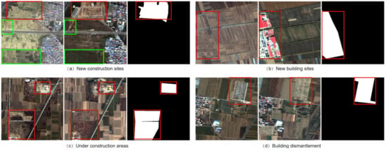
Figure 1.
The illustration of the change detection problem. The images of each sub-figure are corresponding to images at and and the given change label mask. (a–d) are the examples of four different kinds of urban construction-related changes in our dataset. The red boxes bound the urban construction-related change areas and the green boxes mark the change areas we do not consider.
As shown in Figure 1, the left two images of each sub-figure are captured on and , respectively. The right one is their corresponding pixel-wise label mask, which labels the changes related to urban construction. The target urban construction-related changes can be comprehended as follow:
- New construction sites (Figure 1a). It is worth noting that the construction sites are always featured by the blue dust protection canvas (white box a) and the building construction traces (white box b).
- New building sites (Figure 1b). This indicates that new buildings are built up in this area.
- Under construction areas (Figure 1c). This means that this area is under construction during the time period.
- Building dismantlement(Figure 1d). If buildings are dismantled during the time period in some areas, it is also considered as a changed area in our task setting.
It should be mentioned that although geographical changes also happen in some areas, such as the farmland changes (bounded by green boxes), we do not take these changes into consideration, which is essentially different from some other researches. On the one hand, the datasets used in [24,46], such as Yellow River dataset and urban Mexico dataset, simply search for the significant surface changes instead of high-level semantic changes in the time period. On the other hand, although the dataset in [17] considers five kinds of changes, the scale of the dataset (The dataset only contains 13 image pairs with the size of .) prevents it from well training a deep neural network for intelligent detection. Our proposed dataset, however, provides the precondition for applying a deep segmentation network to automatic change detection in an end-to-end manner.
3.2. Proposed Network
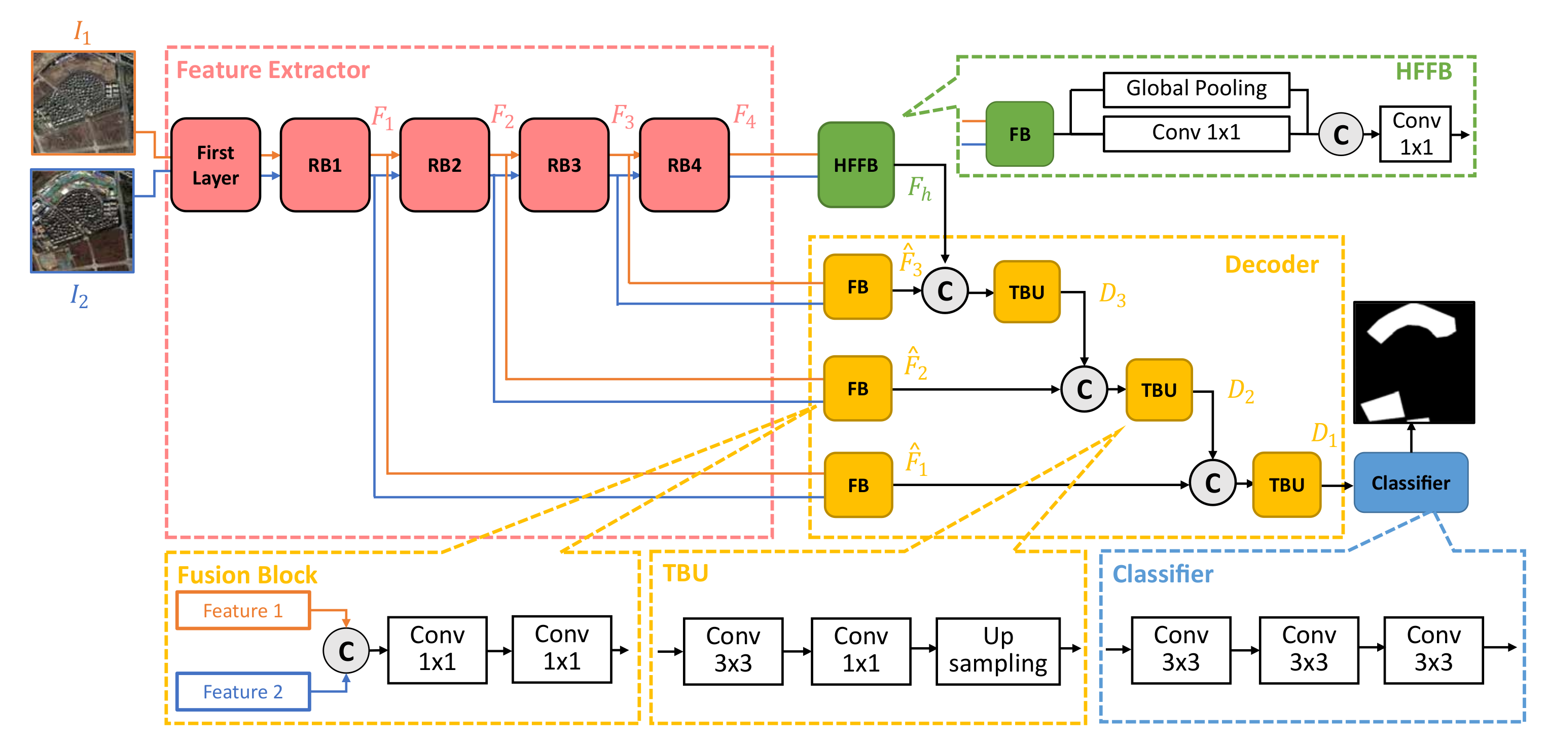
In this subsection, a change detection method based on a deep segmentation network is introduced. We treat the change detection task as a semantic segmentation problem. The network consists of a feature extractor, a high-level feature fusion block (HFFB), a decoder and a pixel classifier. In general, the feature extractor transforms a pair of images, and , to a feature space where they have more consistent representations by gradually reducing the spatial resolution and increasing the number of feature maps. Then the decoder works as an up-sampling network to transform the low-resolution features to high-resolution change predictions. This transformation is achieved by efficiently blending the change information from high-level layers with fine details from bottom layers. The overall illustration and the size of corresponding feature maps are provided in Figure 2 and Table 1.
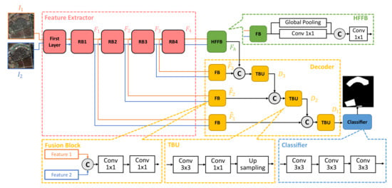
Figure 2.
Illustration of the architecture of the proposed network. It mainly consists of four parts: Feature extractor (in siamese architecture), HFFB, Decoder and Pixel classifier.

Table 1.
Feature map size.
3.2.1. Feature Extractor
Similar to many previous works [44,45,47], our model uses ResNet [48] as the backbone of our network, which is responsible for feature extracting from the original image pairs. Motivated by the design in [45], the ResNet backbone involves 4 Residual Blocks (RB) according to the resolutions of the feature maps, where we implement a multi-grid method on the RB4 to enlarge the receptive field of the network. However, different from the [45], the proposed feature extractor is modified to a siamese architecture, which indicates that two images and are fed into the network simultaneously with shared weights. The outputs of each RB are then utilized in deeper layers.
The procedure can be described as follow: The feature extractor first preprocesses two input images and the resulting features are fed into RB1 to generate feature maps by reducing the spatial resolutions while increasing the number of channels. Then the obtained is connected to RB2 for subsequent feature extraction to calculate . This process is repeated when two images pass all 4 RBs. The resulting features, , are then prepared for detecting the change areas on pixel-level.
3.2.2. High-Level Feature Fusion
Although atrous spatial pyramid pooling (ASPP) [44] has shown its strong ability in many segmentation architectures [44,45,47], we find that the ASPP can negatively affect the network performance in our change detection tasks. Different from the semantic segmentation tasks on traditional datasets, such as the Cityscapes [49], within which the images are all in a perspective view and always contain the same kind of object with an arbitrary scale, all image pairs in our change detection dataset are not in a perspective view, which leads to that all objects with the same category in the images are approximately with the same scale.
Therefore, we directly use a global average pooling layer and a Conv layer (In this paper, a Conv layer includes a convolutional layer with kernel of , a batch normalization layer [50] and a ReLu layer [51].) to conduct the high-level representation fusion. We call the proposed block a High-level feature fusion block (HFFB). Ablation studies further demonstrate that the network with HFFB is superior to the one with ASPP in the change detection tasks.
As shown in Figure 2, the HFFB has a fusion block (FB, which is introduced in the next subsection.) and 2 parallel data paths including (a) one global average pooling layer, and (b) one Conv layer (with 256 filters). The HFFB firstly applies a FB to compress the . Then it extracts the high-level change features. The resulting features are concatenated and compressed to by another Conv layer for later use.
3.2.3. Decoder
As the feature extractor and HFFB have already generated the features from low to high semantic levels ( and ), the decoder is responsible for detecting whether changes happen between the image pairs on the pixel level. The proposed decoder (Figure 2) consists of FBs and transition up-sampling blocks (TBU). It provides a generic way to refine the coarse high-level semantic change information by exploiting low-level features. Generally, the coarse features from deeper layers (such as ) contain the change information including the existence and the location of the change areas. However, this is not enough for many change detection tasks. We thus implement the decoder shown in Figure 2 to further recover fine details of the change areas which are lost due to the down-sampling operations in the feature extractor.
The architecture of FB is shown in Figure 2. The feature maps from and are directly concatenated by the FB. A Conv layer is then applied to fuse these features. We further implement another Conv layer to reduce the channel number of the resulting fused feature maps. This balances the relative influence of the two data paths and allows to blend the two representations by a subsequent simple concatenation, where the outputs of FB with as input are denoted as , where .
After concatenation of the feature maps from different levels, a TBU is utilized for blending the coarse change areas and their fine details. After the feature blending, TBU then up-samples the resulting features with bilinear interpolation to ensure that the spatial resolution of the features are the same as the low-level representations, which is necessary for subsequent detail recovering.
The feature fusion in the decoder can be described as follow: The decoder firstly blends the feature maps in by a FB, and generates . Then we concatenate and . The obtained features are fed to a TBU to generate , where the up-sampling operation ensures that has the same spatial resolution as calculated by . is then concatenated with and fed to another TBU to generate . The blending procedure is recursively repeated along the decoder data path with connections with the output of each RB. The final TBU generates , which contains all change information on different semantic levels (global information and details).
3.2.4. Pixel Classifier
A fully convolutional sub-network is implemented as a pixel classifier (Figure 2) to generate the final dense predictions. We a two Conv layers and one Conv layer to predict scores for each pixel. Two dropout layers [52] with ratio 0.5 and 0.1, respectively, are also implemented in the second Conv layer and the final Conv layer.
The cross-entropy (CE) loss for binary classification is implemented as the loss function. Due to that the number of pixels for unchanged areas is much more than that of the changed areas in the dataset, we introduce a weighting factor for the positive and negative classes. In this paper, can be set by inverse class frequency. We denote as network’s estimated probability for the changed pixel and define analogously to . We write the -balanced CE loss as
Furthermore, the target ground truths are down-sampled to the size of the output features. We find this operation important, since it removes many high-frequency labeling noises and results in back-propagation of high quality information. In our experiments, the original ground truths are with the size of , and the output of our network is . We down-sample the label mask to instead of up-sampling the final logits to conduct the back-propagation.
4. Experiments
4.1. Dataset Description
We give a brief introduction to the proposed change detection dataset in this subsection. The proposed dataset contains 876 optical remote sensing image pairs with the size of for each image. Their corresponding label masks marking the urban construction-related change areas are also provided with the same size of each image. Some samples of this dataset are shown in Figure 1. The code and dataset can be available online: https://github.com/yangle15/Deep-Siamese-Networks-based-Change-Detection (accessed on 26 July 2021).
4.2. Implementation Details
The implementation details of our model are described as follows:
Learning rate policy: We train our models using a step learning rate policy. Specifically, the initial learning rate will be multiplied by after every 20 epoch. The initial learning rate is set to . We use momentum of 0.9 and weight decay of . The total number of training epochs is set as 90 in all experiments.
Data augmentation: We apply data augmentation by randomly left-right and up-down flipping with the probability of 0.5 during training to enhance the robustness of our model.
Batch normalization: Our added modules on top of ResNet all include batch normalization parameters [50]. Since a large batch size is required to train batch normalization parameters, we employ synchronized batch normalization in our network, where the batch size of 8 is provided in the experiments.
Up-sampling logits: As we have described before, we down-sample the target ground truths to the size of output feature maps of the network instead of up-sampling the outputs, i.e., the provided label masks are down-sampled from to in the experiments.
Weighting factors: We weight the loss terms for changed and unchanged pixels with factors of 0.5223 and 11.7198, respectively, by inverse class frequency.
4.3. Evaluation Criteria
We represent the change detection results in the form of a binary map in which pixel value 1 (white) and 0 (black) denote changed and unchanged regions, respectively. We further consider the changed pixels as positive samples and unchanged ones as negative ones. The following quantitative analysis is provided to evaluate the performance of different change detection methods.
(1) Confusion Matrix: We first calculate the confusion matrix of the positive samples, including false negative (FN), false positive (FP), true negative (TN) and true positive (TP), where FN represents the number of changed pixels that are classified as unchanged ones, and TP denotes the number of pixels correctly classified as changed ones.
(2) Acc: To evaluate the overall performance of methods, the pixel classification accuracy (Acc) is provided, which is calculated by
(3) cIoU: The intersection over union (IoU) rate is a commonly used metric in semantic segmentation tasks to evaluate the effectiveness of a method in segmenting a certain object. Therefore, we provide the intersection over union rate of the changed pixels (cIoU) of different methods in experiments. cIoU can be calculated by
(4) Precision, Recall and F-score: Precision and Recall are import measurements for the performance of a change detection model. Precision and Recall can be calculated by
The Precision-Recall curve (PR curve) is also provided to illustrate the performance of different change detection methods. A high quality curve should have a tendency of touching the top-right corner of the coordinate.
F-score is also provided to evaluate the model, which can be represented as
F-score equally pay attention to the precision and recall, and provides an overall measurement for the performance of a change detection model. A higher F-score represents a better performance.
(5) ROC and AUC: We also evaluate the quality of the final result by using the receiver operating characteristics (ROC) plot, which is depicted by TP rate (TPR) and FP rate (FPR).
The better the ROC curve is, the closer it should be to the top-left corner of the coordinate. Furthermore, the area under the ROC curve (AUC) provides a numerical measure for the prediction result, where the AUC of a ideal result should be equal to 1.
4.4. Change Detection Results on Deep Segmentation Networks
4.4.1. Experimental Settings
As the proposed network is based on the deep semantic segmentation networks, in this subsection, we evaluate different segmentation architectures in the change detection task on the proposed dataset. Two different backbones, ResNet101 and ResNet50, are used in our experiments. Our siamese change detection method is compared with popular segmentation networks, including, DeeplabV1 [47], DeeplabV2 [44], DeeplabV3 [45] and Dual-Attention net [53]. Moreover, we compare the results of the Deep Siamese Convolutional Network (denoted as DSCN in our experiments) proposed in [19] and our method to further verify the effectiveness.
To implement the semantic segmentation networks in the change detection task, we modify the number of input channels as 6. Then the image pairs can be fed directly and the change detection task is transformed into a two-class segmentation problem. In the experiments, we apply the same learning rate policy and data augmentation which are utilized in our method for all tested networks. Moreover, we apply the same weighting factors for positive and negative samples to guarantee the algorithms pay the same attention to positive samples. We randomly divide the original dataset into five equal subsets, among which four subsets are used for training and one for test.
4.4.2. Change Detection Results
The experimental results are shown in Table 2. From experimental results, we can conclude the proposed method outperform other semantic segmentation deep networks in general.

Table 2.
Change detection performance. *: Since the DA-net does not perform well on our change detection task, we do not provide the ROC and AUC of DA-net. -: Since DSCN does not generate the results through a softmax layer, we can not compare the AUC.
Compared with other segmentation networks, the proposed method can achieve higher accuracy, cIoU and F-score, which demonstrates the effectiveness of our method in our change detection task. From the distinguished performance of our method, we can infer that utilizing the siamese architecture in the segmentation network helps improve the network performance in change detection tasks significantly. Although semantic segmentation tasks and change detection problems have some characteristics in common, the difference between these two problems limits the performance of segmentation networks applied in change detection tasks. To cope with the change detection problem under the segmentation setting, the image pairs should be directly fed into the network to generate the feature maps. This can result in the mixing up of important features in the early layers, which confuses the network and restricts the performance of segmentation networks in change detection problems. Different from segmentation architectures, the siamese structure in the proposed network enables the network to learn the similarity between the image pairs as well as to find the target change areas, which leads to improvement of performance.
We further find that the performance of DA-net is quite unsatisfied. It achieves a low cIoU and F-score even with a relatively high pixel classification accuracy. As the number of negative samples (unchanged pixels) is much larger than the positive ones (changed pixels), we indicate that DA-net has difficulty in addressing the imbalanced data problem even provided the weighting factors during the training. The Fully Convolutional Network (FCN) [40] suffers this problem more heavily in our experiments, It classifies all the pixels as negative and can not be implemented in our change detection task with the provided weight factors.
Although the Deep Siamese Convolutional Network in [19] also utilizes the siamese architecture to conduct change detection tasks, our method is obviously superior to it in the experiments. Since DSCN is designed based on a relatively shallow network, it has difficulty in modeling the change features under such a large dataset. Furthermore, with a much deeper network, the proposed methods further apply the techniques in semantic segmentation, such as atrous convolution and skip connection, which strengthens our method to detect the target change areas from global and regional view, and thus results in a better performance in the experiments.
4.4.3. ROC and PR Curves
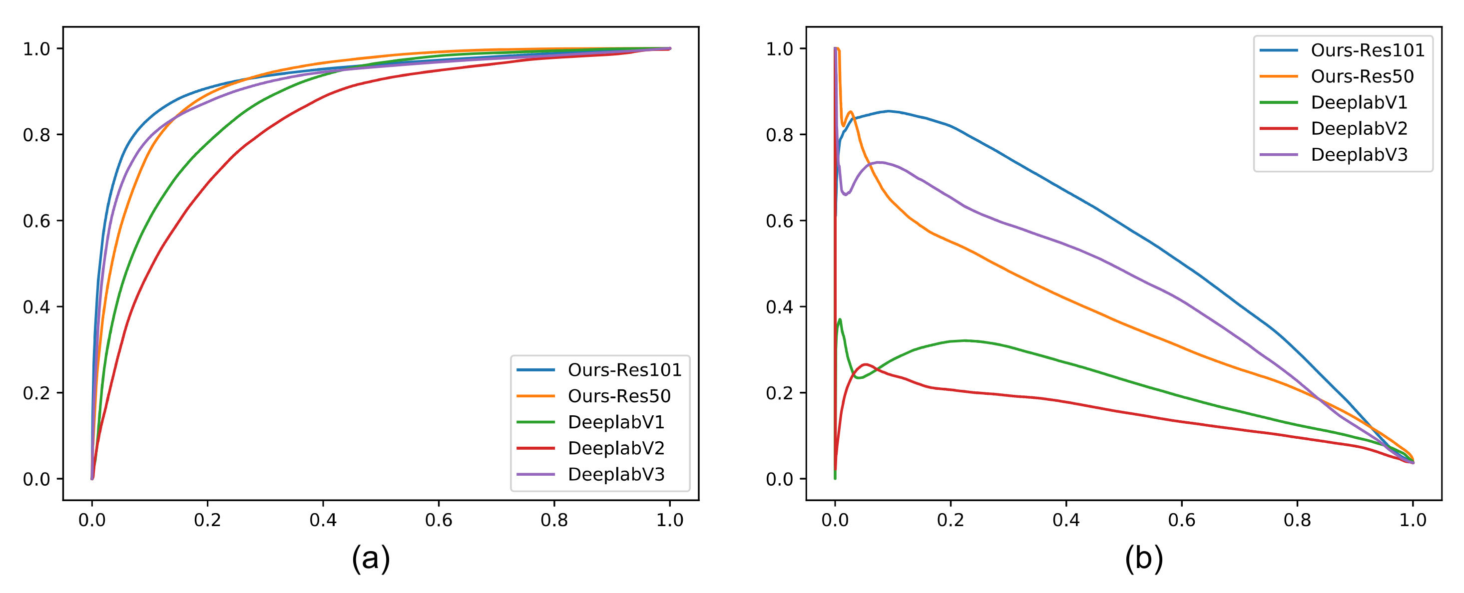
Figure 3 exhibits the PR and ROC curves of different methods on the proposed dataset, respectively. The PR curve of a better result is closer to the top-right corner of the coordinate system, while the ROC curve of a better result is closer to the top-left corner. From the ROC and PR curves, we conclude that the proposed methods (based on Res101 and Res50) can achieve competitive results in change detection tasks, which demonstrates the effectiveness of the proposed methods.
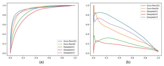
Figure 3.
ROC (a) and PR (b) curves of different methods on the proposed dataset.
It is interesting to find that the proposed method based on Res50 can be superior to the one based on Res101 when the recall is higher than 0.9. This means that the ResNet101 based model will have a higher cost to accurately classify a positive sample while the high recall rate has been achieved, indicating that larger models will perform more aggressively to recognize positive samples in the imbalanced data classification tasks under a high recall rate.
Moreover, all methods in Figure 3a seem to perform well when we use ROC as our evaluation metric (especially DeeplabV3). However, as the samples in our experiments are highly imbalanced (much more negative samples), ROC curves can be a misleading indication of model performance. With imbalanced data, it becomes pretty easy for any model to correctly predict negatives. Because the ROC curve in part plots false positive rates that are calculated with the resulting large number of true negatives in the denominator, by that metric all methods will seem to be doing pretty well. Since it becomes easier to predict negatives as they become more common, evaluating false positive rates with the imbalanced dataset might not be that informative. Therefore, we believe that the PR curve is a more reasonable metric to evaluate each model in our experiments (Figure 3b), where we see that the proposed model based on Res101 outperforms other methods.
4.5. Comparison with the SCCN
Although the classical change detection algorithms can also perform well in some change detection tasks, they have difficulty in detecting specific changes. On one hand, large scale change detection dataset with corresponding labels is a necessary precondition to detect specific changes. On the other hand, the method should have the ability to handle such a large scale dataset, which limits the implementation of classical change detection methods on the proposed large scale change detection tasks.
In this subsection, we provide experiments to evaluate the performance of the proposed method and a traditional change detection method, the classical symmetric convolutional coupling network (SCCN) [46]. Following the experiment setting in [46], we conduct the change detection task on just one image pair and the corresponding label mask, which are shown in Figure 4a,b. In our experiments, we set the sizes of all convolution kernels to and specify 3 coupling layers for each side of the SCCN with the same number of 20 feature maps at each hidden layer. We further set as 0.1, 0.15 and 0.17 for SCCN in the experiments. The results of SCCN with different and the proposed method are shown in Table 3 and visualized in Figure 4.

Figure 4.
The change detection task on one image pair with the proposed method and the SCCN. (a) The given image pair. (b) The label mask. (c) The result of our method. (c–e) are the results of the SCCN with , respectively.

Table 3.
Detection results on one image-pair.
From the experiments, we see that the proposed method is superior to the SCCN on the given change detection task. For the SCCN, large makes the algorithm aggressive in classifying the pixels as positive, especially when (nearly all pixels are classified to changed ones). This meets the demonstrations in [46]. Moreover, the SCCN tends to detect the changes on texture-level (such as the ground surface changes) instead of the target semantic changes (urban construction-related changes). Thus, we can conclude that the SCCN has difficulty in the proposed change detection task, even it has a distinguished performance on many other traditional change detection datasets. However, our method can detect the target changed areas automatically on a high semantic level with satisfied performance (the detection results of our model is nearly close to the original label mask), from which we can conclude that the proposed method can conduct change detection tasks with higher accuracy in a more intelligent way.
4.6. Ablation Study
4.6.1. The Scale of the Dataset
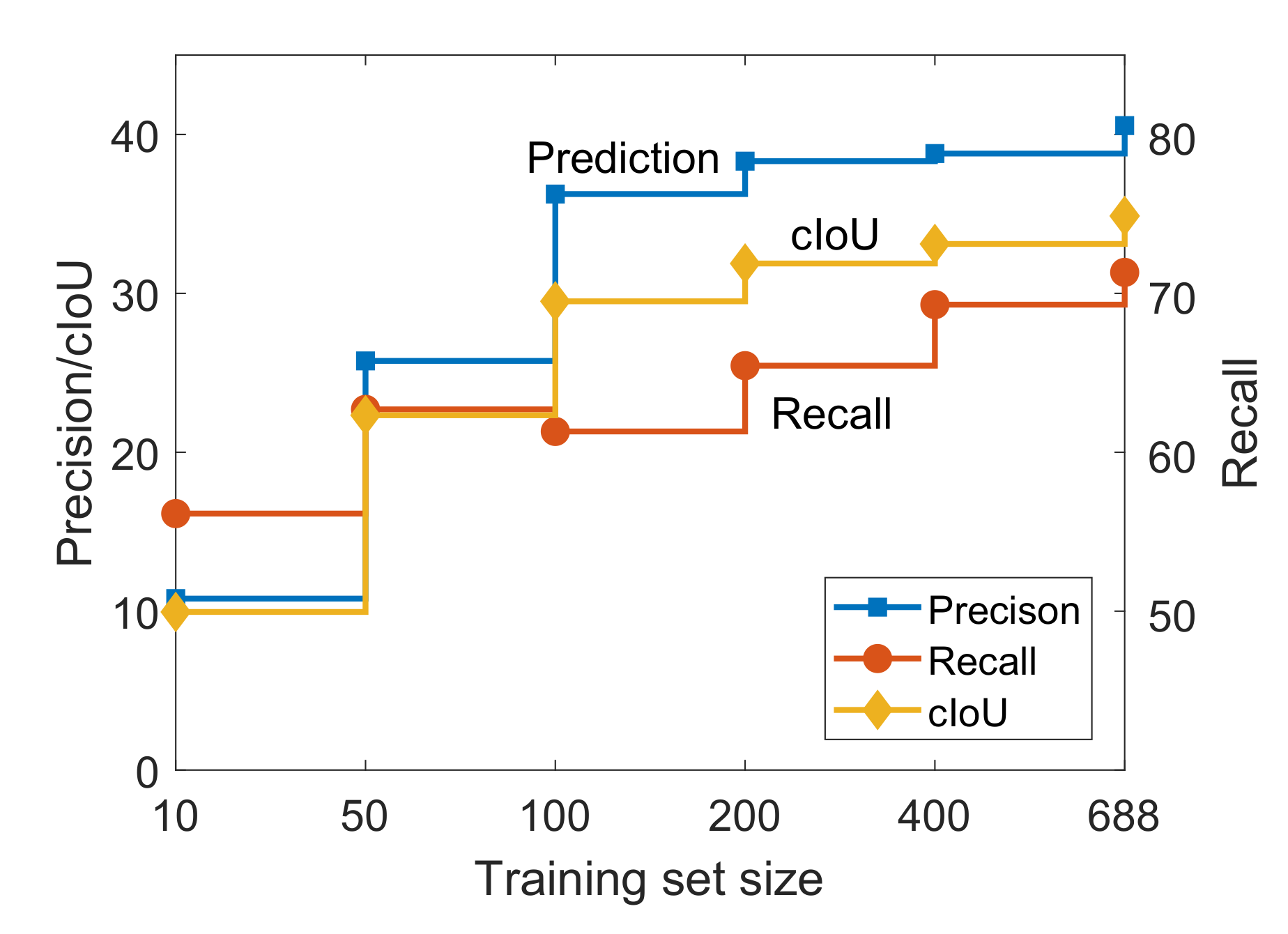
As the insufficiency of the change detection dataset can limit the models to explore the features of the changed areas, we study the impact of the number of image pairs on the performance of change detection methods. In the experiments, we randomly select a given number of image pairs to train the proposed network. The experimental results are shown in Table 4 and Figure 5.

Table 4.
Ablation study for dataset scale.
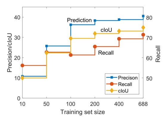
Figure 5.
The performance of the network vs. the training set size.
From the results, we can demonstrate that the dataset with larger scale can provide a more accurate prediction in change areas. Due to the deep segmentation network can only be driven with large scale data, the performance of the network has an obvious drop when the number of image pairs decreases. We notice that the network performs poorly when the number of image pairs is 10, which is the number of image pairs in many other change detection datasets. Therefore, the study indicates the importance of the proposed dataset.
4.6.2. The Network Architecture
In this section, we conduct the ablation study to reveal the effectiveness of each part of the proposed network. The performance is evaluated by five metrics, including cIoU, Accuracy (Acc), Precision (P), Recall (R) and F-score (F).
Siamese architecture: As one of our novelty is to modify the semantic segmentation network to siamese architecture for change detection task, the benefits of this modification is studied in the experiments. The proposed method without siamese architecture is conducted by changing the number of input channels of the network from 3 to 6, which is similar to other semantic segmentation networks in the previous experiments. The experimental results are shown in Table 5. As we can see, implementing the siamese architecture in our deep network significantly improves the performance of the network in change detection tasks. Although the Recall rate drops from 75.19 to 71.32 for Res101 based model, and from 80.34 to 76.23 for Rese50 based model, the cIoU and precision for Res101 based model increase from 27.84 to 34.87 and from 30.56 to 40.56, respectively. Other metrics, such as Pixel accuracy and F-score also have remarkable increases.

Table 5.
Ablation study for siamese architecture. √ mean that the Decoder fuses the corresponding features to generate the final Predictions.
Under the classical semantic segmentation architecture, the image pairs are directly fed into the deep network, which can mix-up the features from two images and confuse the network in detecting change areas. However, different from the classical segmentation network, the proposed methods with siamese architecture processes two given images separately with the shared weights, which projects the representations of two images in the original feature space to a new feature space, where the changed areas are far apart and the unchanged areas are closer. This results in a significant improvement in performance.
Skip connection: The skip connection in semantic segmentation is curial for accurate detection, which refines the detailed information of the target objects. In this experiment, we explore that whether the skip connection in the proposed method has the same refine function. As our network utilizes all the low-level features (, and ) in detecting the change areas, we evaluate the network removing the skip connections. The results are shown in Table 6.

Table 6.
Ablation study for skip connection (RES101). √ mean that the Decoder fuses the corresponding features to generate the final Predictions.
Because the skip connection to the early layer provides a generic mean to refine the coarse high-level semantic change information () by exploiting low-level features. the network further recovers fine details of the change areas which are lost due to the downsampling operation in the feature extractor. Without the detailed information from the early layers, the network can only roughly detect the existence and location of the changes. Our network with skip connection accurately refines the detection results, which consequently leads to the improvement of the network performance.
Moreover, we visualize the function of the skip connection in Figure 6. We can see that although the network without skip connection can detect the existence and location of the change areas, it misses the detailed information of the areas. Our method, with the refinement by the skip connection, can detect the changing area with higher accuracy and more precise details.
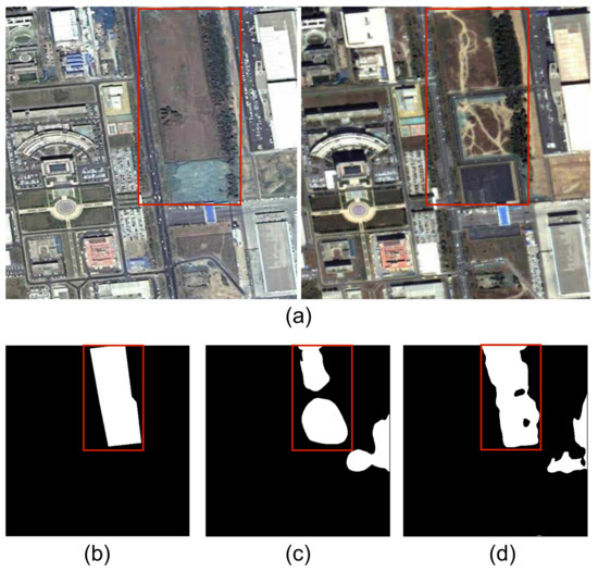
Figure 6.
Visualization of the function for the skip connection. (a) the optical remote sensing image pair. (b) The label mask. (c) The result without skip connection. (d) The result with skip connection.
Coarse label: The influence of the downsampling of the ground truths for our network is further tested. In our ablation study, the Coarse Label setting represents that we down-sample the ground truths during the training procedure. We further test the results when we up-sample the network output to the size of to conduct the back-propagation. The experimental results are shown in Table 7.

Table 7.
Ablation study for skip connection (RES101). √ mean that the Decoder fuses the corresponding features to generate the final Predictions.
In [45] it is claimed that keeping the ground truths intact and instead up-sampling the final logits of the network is important, since down-sampling the ground truths remove the fine annotations resulting in no back-propagation of details. However, we find it is not suitable for our network. The network with coarse labels is slightly superior to the one with detailed labels in our ablation study, which might be because down-sampling the ground truths removes many high-frequency labeling noises resulting in back-propagation of high quality details.
4.7. Visualization Results
In this subsection, we visualize the change detection results by covering the original image pairs with the real change labels and the predicted change labels, respectively. In the visualization results, the top two images of each sub-figure are the image pairs covered with the real labels, while the bottom two are the image pairs masked by the predicted labels. All the visualization results are obtained from the models based on Resnet101.
4.7.1. Qualitative Results
We provide qualitative visual results of our best change detection model in Figure 7. As shown in the figure, our model can detect the urban construction-related change areas accurately. From the visualization results, we see that the shapes of the predicted change areas are roughly the same as the real change areas, except for some detailed margins. Moreover, Figure 7e shows that our detection model can identify the target change areas regardless of the size of the change areas.

Figure 7.
Qualitative change detection results. The top two images of (a–e) are the image pairs covered with the real labels, while the bottom two are the image pairs masked by the predicted labels.
4.7.2. Argued Detection Patterns
There are also some argued detection patterns, which are showed in Figure 8. In the proposed dataset, we find that there exist some urban construction-related areas which are not labeled in the provided label masks (bounded by blue boxes in Figure 8), which might be due to the manual labeling error. However, as the proposed detection model can find the intrinsic features of the change areas, the ignored change areas are also detected in the tasks, which consequently, demonstrates the effectiveness of the proposed model. Furthermore, we can also indicate that the theoretical detection results, including precision and change area cIoU, can be higher than the reported ones.

Figure 8.
Samples of argued detection patterns (a-e). The missing labeled urban-construction-related change areas are bounded by the blue boxes.
4.7.3. Failure Modes
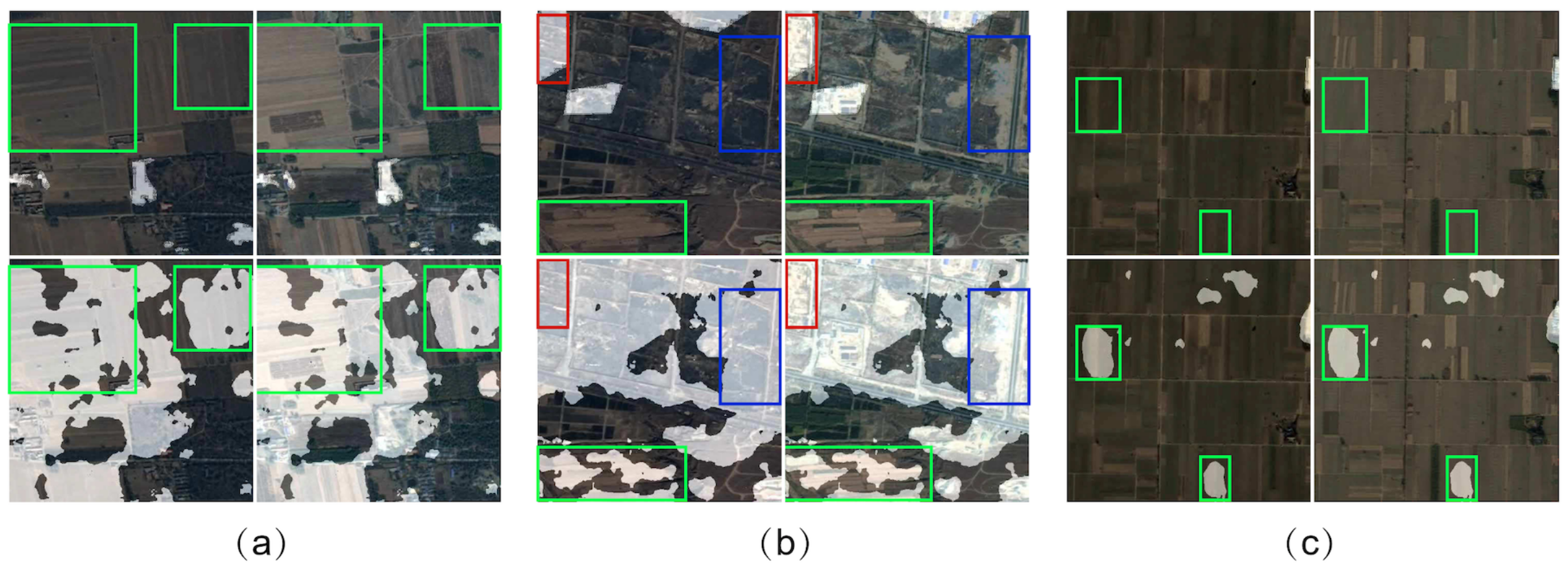
As shown in Figure 9, our model has difficulty in some cases. Some of the farmlands are wrongly classified to the urban construction change areas, which are bounded by green boxes. This might be due to the ground surface changing usually happens in farmlands. Moreover, the noises in labeling might further results in the decent of the performance.
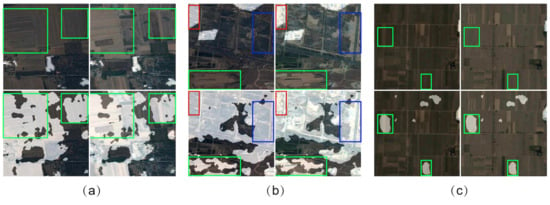
Figure 9.
Samples of failure detection modes (a–c). We use red boxes, blue boxes and green boxes to bound the accurately detected areas, ignored labeled detected areas and wrongly detected areas, respectively.
4.7.4. Comparison with Other Segmentation Models
The visualization results of different semantic segmentation results are further provided in Figure 10. From labels, we see that there are three changed areas. The results in (b) and (c) show that a wide range of areas is detected as changed areas. This indicates that the DeeplabV1 and DeeplabV2 are sensitive to the changed areas but have problems accurately predicting the locations of changed areas, which results in aggressive detection results. The multi-grid atrous convolutions in DeepLabV3 make the predictions more accurate, but one changed area is missing in the results. Overall, due to the application of the siamese architecture, our method detects all change areas and achieves better detection performance.

Figure 10.
Visualization results of the proposed method and other sematic segmentation models. (a) Our model. (b) DeeplabV1. (c) DeeplabV2. (d) DeeplabV3.
5. Conclusions
In this paper, we proposed a change detection dataset with 862 optical remote sensing image pairs. Different from existing datasets, which usually define all ground surface changes as change areas, the proposed dataset only focuses on urban construction-related changes while ignores other changes. Such a specific change detection is much more challenging and with more practical value compared with traditional change detection tasks. To deal with the aforementioned change detection problem, we further designed a novel change detection method based on a deep siamese semantic segmentation network. Experiments show that the proposed network is superior to other methods in the change detection problem. Future work mainly includes that building deep learning based change detection methods in a semi-supervised or unsupervised manner.
Author Contributions
All authors collaborated to conduct this work; G.H. conceived and designed the content of this paper; L.Y. and Y.C. designed the deployed the proposed network; Y.C. processed the remote sensing images and L.Y. contribued to the experiments. L.Y. and Y.C. wrote the manuscript. S.S. and F.L. reviewed and revised the manuscript. All authors have read and agreed to the published version of the manuscript.
Funding
This research was supported by National Natural Science Foundation of China: U1903213, National Natural Science Foundation of China: 41427806 and Key Projects of Ministry of Science and Technology of China: 2016YFB1200203.
Institutional Review Board Statement
Not applicable.
Informed Consent Statement
Not applicable.
Data Availability Statement
Restrictions apply to the availability of these data. Data was obtained from the PIESAT Information Technology Co., Ltd., and are available from the authors with the permission of the PIESAT Information Technology Co., Ltd.
Acknowledgments
The research data is provided by the PIESAT Information Technology Co., Ltd.
Conflicts of Interest
The authors declare no conflict of interest.
Abbreviations
The following abbreviations are used in this manuscript:
| DI | Difference Image | GSD | Ground Sampling Distance |
| HFFB | High-level Feature Fusion Block | RB | Residual Block |
| ASPP | Astrous Spatial Pyramid Pooling | FB | Fusion Block |
| TBU | Transition Up-sampling Block | CE | Cross Entropy |
References
- Singh, A. Review article digital change detection techniques using remotely-sensed data. Int. J. Remote Sens. 1989, 10, 989–1003. [Google Scholar] [CrossRef] [Green Version]
- Radke, R.J.; Andra, S.; Al-Kofahi, O.; Roysam, B. Image change detection algorithms: A systematic survey. IEEE Trans. Image Process. 2005, 14, 294–307. [Google Scholar] [CrossRef]
- Yang, J.; Weisberg, P.J.; Bristow, N.A. Landsat remote sensing approaches for monitoring long-term tree cover dynamics in semi-arid woodlands: Comparison of vegetation indices and spectral mixture analysis. Remote Sens. Environ. 2012, 119, 62–71. [Google Scholar] [CrossRef]
- Xian, G.; Homer, C. Updating the 2001 National Land Cover Database impervious surface products to 2006 using Landsat imagery change detection methods. Remote Sens. Environ. 2010, 114, 1676–1686. [Google Scholar] [CrossRef]
- Argüello, F.; Heras, D.B.; Garea, A.S.; Quesada-Barriuso, P. Watershed Monitoring in Galicia from UAV Multispectral Imagery Using Advanced Texture Methods. Remote Sens. 2021, 13, 2687. [Google Scholar] [CrossRef]
- Li, X.; Lin, H.; Long, J.; Xu, X. Mapping the Growing Stem Volume of the Coniferous Plantations in North China Using Multispectral Data from Integrated GF-2 and Sentinel-2 Images and an Optimized Feature Variable Selection Method. Remote Sens. 2021, 13, 2740. [Google Scholar] [CrossRef]
- Tison, C.; Nicolas, J.M.; Tupin, F.; Maître, H. A new statistical model for Markovian classification of urban areas in high-resolution SAR images. IEEE Trans. Geosci. Remote Sens. 2004, 42, 2046–2057. [Google Scholar] [CrossRef]
- Bovolo, F.; Bruzzone, L. A detail-preserving scale-driven approach to change detection in multitemporal SAR images. IEEE Trans. Geosci. Remote Sens. 2005, 43, 2963–2972. [Google Scholar] [CrossRef]
- Zheng, Y.; Zhang, X.; Hou, B.; Liu, G. Using combined difference image and k-means clustering for SAR image change detection. IEEE Geosci. Remote Sens. Lett. 2013, 11, 691–695. [Google Scholar] [CrossRef]
- Ma, J.; Gong, M.; Zhou, Z. Wavelet fusion on ratio images for change detection in SAR images. IEEE Geosci. Remote Sens. Lett. 2012, 9, 1122–1126. [Google Scholar] [CrossRef]
- Bovolo, F.; Bruzzone, L. A theoretical framework for unsupervised change detection based on change vector analysis in the polar domain. IEEE Trans. Geosci. Remote Sens. 2006, 45, 218–236. [Google Scholar] [CrossRef] [Green Version]
- Bovolo, F.; Marchesi, S.; Bruzzone, L. A framework for automatic and unsupervised detection of multiple changes in multitemporal images. IEEE Trans. Geosci. Remote Sens. 2011, 50, 2196–2212. [Google Scholar] [CrossRef]
- Bock, M.; Xofis, P.; Mitchley, J.; Rossner, G.; Wissen, M. Object-oriented methods for habitat mapping at multiple scales–Case studies from Northern Germany and Wye Downs, UK. J. Nat. Conserv. 2005, 13, 75–89. [Google Scholar] [CrossRef]
- Chen, G.; Zhao, K.; Powers, R. Assessment of the image misregistration effects on object-based change detection. ISPRS J. Photogramm. Remote Sens. 2014, 87, 19–27. [Google Scholar] [CrossRef]
- Wang, B.; Choi, S.; Byun, Y.; Lee, S.; Choi, J. Object-based change detection of very high resolution satellite imagery using the cross-sharpening of multitemporal data. IEEE Geosci. Remote Sens. Lett. 2015, 12, 1151–1155. [Google Scholar] [CrossRef]
- Liu, J.; Gong, M.; Qin, A.; Tan, K.C. Bipartite Differential Neural Network for Unsupervised Image Change Detection. IEEE Trans. Neural Netw. Learn. Syst. 2020, 31, 876–890. [Google Scholar] [CrossRef]
- Benedek, C.; Sziranyi, T. Change Detection in Optical Aerial Images by a Multilayer Conditional Mixed Markov Model. IEEE Trans. Geosci. Remote Sens. 2009, 47, 3416–3430. [Google Scholar] [CrossRef] [Green Version]
- Gong, M.; Zhao, J.; Liu, J.; Miao, Q.; Jiao, L. Change detection in synthetic aperture radar images based on deep neural networks. IEEE Trans. Neural Networks Learn. Syst. 2015, 27, 125–138. [Google Scholar] [CrossRef]
- Zhan, Y.; Fu, K.; Yan, M.; Sun, X.; Wang, H.; Qiu, X. Change detection based on deep siamese convolutional network for optical aerial images. IEEE Geosci. Remote Sens. Lett. 2017, 14, 1845–1849. [Google Scholar] [CrossRef]
- Li, X.; Deng, J.; Fang, Y. Few-Shot Object Detection on Remote Sensing Images. IEEE Trans. Geosci. Remote. Sens. 2021. [Google Scholar] [CrossRef]
- Bazi, Y.; Bruzzone, L.; Melgani, F. An unsupervised approach based on the generalized Gaussian model to automatic change detection in multitemporal SAR images. IEEE Trans. Geosci. Remote Sens. 2005, 43, 874–887. [Google Scholar] [CrossRef] [Green Version]
- Hu, H.; Ban, Y. Unsupervised change detection in multitemporal SAR images over large urban areas. IEEE J. Sel. Top. Appl. Earth Obs. Remote Sens. 2014, 7, 3248–3261. [Google Scholar] [CrossRef]
- Celik, T. Unsupervised change detection in satellite images using principal component analysis and k-means clustering. IEEE Geosci. Remote Sens. Lett. 2009, 6, 772–776. [Google Scholar] [CrossRef]
- Gong, M.; Zhou, Z.; Ma, J. Change detection in synthetic aperture radar images based on image fusion and fuzzy clustering. IEEE Trans. Image Process. 2011, 21, 2141–2151. [Google Scholar] [CrossRef]
- Gong, M.; Su, L.; Jia, M.; Chen, W. Fuzzy clustering with a modified MRF energy function for change detection in synthetic aperture radar images. IEEE Trans. Fuzzy Syst. 2013, 22, 98–109. [Google Scholar] [CrossRef]
- Chen, K.; Huo, C.; Zhou, Z.; Lu, H. Unsupervised change detection in SAR image using graph cuts. In Proceedings of the IGARSS 2008-2008 IEEE International Geoscience and Remote Sensing Symposium, Boston, MA, USA, 8–11 July 2008; Volume 3, pp. III–1162. [Google Scholar]
- Moser, G.; Serpico, S.B. Unsupervised change detection with high-resolution SAR images by edge-preserving Markov random fields and graph-cuts. In Proceedings of the 2012 IEEE International Geoscience and Remote Sensing Symposium, Munich, Germany, 22–27 July 2012; pp. 1984–1987. [Google Scholar]
- Miron, A.; Badii, A. Change detection based on graph cuts. In Proceedings of the 2015 International Conference on Systems, Signals and Image Processing (IWSSIP), London, UK, 10–12 September 2015; pp. 273–276. [Google Scholar]
- Bazi, Y.; Melgani, F.; Al-Sharari, H.D. Unsupervised change detection in multispectral remotely sensed imagery with level set methods. IEEE Trans. Geosci. Remote Sens. 2010, 48, 3178–3187. [Google Scholar] [CrossRef]
- Chen, G.; Weng, Q.; Hay, G.J.; He, Y. Geographic Object-based Image Analysis (GEOBIA): Emerging trends and future opportunities. GIScience Remote Sens. 2018, 55, 159–182. [Google Scholar] [CrossRef]
- Im, J.; Jensen, J.; Tullis, J. Object-based change detection using correlation image analysis and image segmentation. Int. J. Remote Sens. 2008, 29, 399–423. [Google Scholar] [CrossRef]
- Silveira, E.M.d.O.; Mello, J.M.d.; Acerbi Júnior, F.W.; Carvalho, L.M.T.d. Object-based land-cover change detection applied to Brazilian seasonal savannahs using geostatistical features. Int. J. Remote Sens. 2018, 39, 2597–2619. [Google Scholar] [CrossRef]
- Mou, L.; Bruzzone, L.; Zhu, X.X. Learning spectral-spatial-temporal features via a recurrent convolutional neural network for change detection in multispectral imagery. IEEE Trans. Geosci. Remote Sens. 2018, 57, 924–935. [Google Scholar] [CrossRef] [Green Version]
- Song, A.; Choi, J.; Han, Y.; Kim, Y. Change Detection in Hyperspectral Images Using Recurrent 3D Fully Convolutional Networks. Remote Sens. 2018, 10, 1827. [Google Scholar] [CrossRef] [Green Version]
- Lei, T.; Zhang, Q.; Xue, D.; Chen, T.; Meng, H.; Nandi, A.K. End-to-end Change Detection Using a Symmetric Fully Convolutional Network for Landslide Mapping. In Proceedings of the ICASSP 2019-2019 IEEE International Conference on Acoustics, Speech and Signal Processing (ICASSP), Brighton, UK, 12–17 May 2019; pp. 3027–3031. [Google Scholar]
- Li, X.; Yuan, Z.; Wang, Q. Unsupervised Deep Noise Modeling for Hyperspectral Image Change Detection. Remote Sens. 2019, 11, 258. [Google Scholar] [CrossRef] [Green Version]
- Peng, D.; Zhang, Y.; Guan, H. End-to-End Change Detection for High Resolution Satellite Images Using Improved UNet++. Remote Sens. 2019, 11, 1382. [Google Scholar] [CrossRef] [Green Version]
- Xu, Q.; Chen, K.; Zhou, G.; Sun, X. Change Capsule Network for Optical Remote Sensing Image Change Detection. Remote Sens. 2021, 13, 2646. [Google Scholar] [CrossRef]
- Chen, H.; Wu, C.; Du, B.; Zhang, L.; Wang, L. Change detection in multisource VHR images via deep siamese convolutional multiple-layers recurrent neural network. IEEE Trans. Geosci. Remote Sens. 2019, 58, 2848–2864. [Google Scholar] [CrossRef]
- Long, J.; Shelhamer, E.; Darrell, T. Fully convolutional networks for semantic segmentation. In Proceedings of the IEEE Conference on Computer Vision and Pattern Recognition, Boston, MA, USA, 7–12 June 2015; pp. 3431–3440. [Google Scholar]
- Noh, H.; Hong, S.; Han, B. Learning deconvolution network for semantic segmentation. In Proceedings of the IEEE International Conference on Computer Vision, Boston, MA, USA, 7–12 June 2015; pp. 1520–1528. [Google Scholar]
- Ronneberger, O.; Fischer, P.; Brox, T. U-net: Convolutional networks for biomedical image segmentation. In Proceedings of the International Conference on Medical Image Computing and Computer-Assisted Intervention, Munich, Germany, 5–9 October 2015; pp. 234–241. [Google Scholar]
- Lazebnik, S.; Schmid, C.; Ponce, J. Beyond bags of features: Spatial pyramid matching for recognizing natural scene categories. In Proceedings of the 2006 IEEE Computer Society Conference on Computer Vision and Pattern Recognition (CVPR’06), New York, NY, USA, 17–22 June 2006; Volume 2, pp. 2169–2178. [Google Scholar]
- Chen, L.C.; Papandreou, G.; Kokkinos, I.; Murphy, K.; Yuille, A.L. Deeplab: Semantic image segmentation with deep convolutional nets, atrous convolution, and fully connected crfs. IEEE Trans. Pattern Anal. Mach. Intell. 2017, 40, 834–848. [Google Scholar] [CrossRef] [PubMed]
- Chen, L.C.; Papandreou, G.; Schroff, F.; Adam, H. Rethinking atrous convolution for semantic image segmentation. arXiv 2017, arXiv:1706.05587. [Google Scholar]
- Liu, J.; Gong, M.; Qin, K.; Zhang, P. A deep convolutional coupling network for change detection based on heterogeneous optical and radar images. IEEE Trans. Neural Netw. Learn. Syst. 2016, 29, 545–559. [Google Scholar] [CrossRef]
- Chen, L.C.; Papandreou, G.; Kokkinos, I.; Murphy, K.; Yuille, A.L. Semantic image segmentation with deep convolutional nets and fully connected crfs. arXiv 2014, arXiv:1412.7062. [Google Scholar]
- He, K.; Zhang, X.; Ren, S.; Sun, J. Deep residual learning for image recognition. In Proceedings of the IEEE Conference on Computer Vision and Pattern Recognition, Las Vegas, NV, USA, 27–30 June 2016; pp. 770–778. [Google Scholar]
- Cordts, M.; Omran, M.; Ramos, S.; Rehfeld, T.; Enzweiler, M.; Benenson, R.; Franke, U.; Roth, S.; Schiele, B. The Cityscapes Dataset for Semantic Urban Scene Understanding. In Proceedings of the IEEE Conference on Computer Vision and Pattern Recognition (CVPR), Las Vegas, NV, USA, 27–30 June 2016. [Google Scholar]
- Ioffe, S.; Szegedy, C. Batch Normalization: Accelerating Deep Network Training by Reducing Internal Covariate Shift. In Proceedings of the International Conference on Machine Learning, Lille, France, 6–11 July 2015; pp. 448–456. [Google Scholar]
- Nair, V.; Hinton, G.E. Rectified linear units improve restricted boltzmann machines. In Proceedings of the International Conference on Machine Learning, Haifa, Israel, 21–24 June 2010; pp. 807–814. [Google Scholar]
- Srivastava, N.; Hinton, G.; Krizhevsky, A.; Sutskever, I.; Salakhutdinov, R. Dropout: A simple way to prevent neural networks from overfitting. J. Mach. Learn. Res. 2014, 15, 1929–1958. [Google Scholar]
- Fu, J.; Liu, J.; Tian, H.; Li, Y.; Bao, Y.; Fang, Z.; Lu, H. Dual attention network for scene segmentation. In Proceedings of the IEEE Conference on Computer Vision and Pattern Recognition, Long Beach, CA, USA, 16–20 June 2019; pp. 3146–3154. [Google Scholar]
Publisher’s Note: MDPI stays neutral with regard to jurisdictional claims in published maps and institutional affiliations. |
© 2021 by the authors. Licensee MDPI, Basel, Switzerland. This article is an open access article distributed under the terms and conditions of the Creative Commons Attribution (CC BY) license (https://creativecommons.org/licenses/by/4.0/).


