Joint Design of the Transmit Beampattern and Angular Waveform for Colocated MIMO Radar under a Constant Modulus Constraint

Abstract

In this paper, we investigate the joint design of a transmit beampattern and angular waveform (AW) for colocated multiple-input multiple-output (MIMO) radars. The importance of the AW in the proposed signal processing strategy is first clarified, and then, two optimization models are established, which are aimed at either the power spectral density (PSD) design or the spectral compatibility and similarity design of the AW. There are two main differences between the proposed models and existing models. First, instead of matching a desired template or maximizing the transmit power on specific regions, the transmit beampattern in this paper is optimized to approach several key points, which guarantees the high transmit gain and the flexible adjustment of each beam gain. Second, instead of optimizing the performance of the transmit waveform, only the characteristics of the AW are examined, and they can be constrained quantitatively according to their relationship with the transmit gain. The two models can be unified into the same framework, and an efficient algorithm is proposed to solve the problem under a constant modulus constraint. The convergence of the proposed algorithm is demonstrated, and some improvements to reduce the computational complexity are proposed. Numerical simulations showed that compared to the existing methods, the proposed approach can be used to obtain a higher transmit gain, flexibly adjust each beam gain, and more accurately control the PSD, spectral compatibility, and similarity of the AW. Moreover, numerical simulations showed that, compared to the use of existing methods, the proposed algorithm has higher computational efficiency.

1. Introduction

It is well known that multiple-input multiple-output (MIMO) radars can transmit independent waveforms out of each transmit antenna. Because of this capability, called “waveform diversity”, MIMO radars realize advantages in terms of parameter identifiability, spatial resolution, and transmit beampattern design compared to a standard phased array radar [1,2,3]. MIMO radars are generally categorized into two types according to the distance between the radar antennas, namely distributed MIMO radars [4] and colocated MIMO radars [5]. The former has antennas widely separated in space, which can make use of the spatial diversity of the radar targets, whereas the latter has closely spaced antennas, which can improve the spatial resolution and parameter identifiability and can introduce a greater number of degrees of freedom in the transmit beampattern design.

Both kinds of MIMO radars need a group of waveforms, which is critical for realizing their claimed advantages over their conventional counterparts [6,7,8,9,10,11,12]. To ensure the receiver can distinguish the target returns caused by different transmit waveforms, the transmit waveforms should be orthogonal to each other, even at different mutual delays [6,7,8,9]. Therefore, for MIMO radars, a critical problem is to design nearly orthogonal waveforms with good auto- and cross-correlation properties. There has been extensive work on the design of a set of nearly orthogonal waveforms [7,13,14]. However, for colocated MIMO radars, the transmit beampattern of nearly orthogonal waveforms is omnidirectional, which has a low transmit gain and is more suitable for search modes or acquiring surrounding information [15,16].

By designing a set of correlated waveforms, colocated MIMO radars can also form a directional transmit beampattern with one or more beams, which is more applicable to scenes with multiple targets [17,18]. Much work has been conducted on the design of correlated waveforms to form directional transmit beampattern [10,11,19,20]. In addition to the transmit beampattern, the temporal or spectral properties of the waveforms are also important. Most of the above work considered the constant modulus (CM) constraint because of the requirement for a radiofrequency amplifier. Besides the CM constraint, in [19], the waveforms were required to satisfy the similarity constraint to share the similar ambiguity function (AF) feature with a given reference waveform. In [10], a set of correlated linear frequency modulation (LFM) waveforms was designed to form a desired beampattern. Considering the spectrally crowded environment in [20], the waveforms were optimized to form notches in a certain spatial-frequency region.

It was noted that the above constraints, such as the near orthogonality and similarity constraints, are applied to each waveform from each transmit antenna. However, for the directional transmit beampattern, the radar can only focus on the returns from the beam directions. The angular waveforms (AWs) are defined as the waveforms coherently synthesized from the transmit waveforms into different angular sectors with respect to the transmit array [6,12,21]. Based on the signal processing strategy in [6,22], the AWs in the beam directions play a more important role in the directional transmit beampattern. Therefore, except for the CM constraint, which is the requirement of the hardware, the near orthogonality and similarity constraints are additionally applied to the AWs under the directional transmit beampattern. Some work [21,23,24,25] has investigated the joint design of the transmit beampattern and AWs with good near orthogonality. In this paper, some more complicated scenarios are considered, and some additional constraints are imposed on the AWs.

In this paper, we deal with complicated scenarios from the view of signal processing, e.g., electronic counter-countermeasures (ECCM) and spectrum congestion. Some earlier work dealt with certain complicated scenarios from the perspective of electromagnetic waves. For example, the work in [26] explored the influence of the magnetic field on quantum cascade lasers. The work of [27,28] investigated the performance of a free-space optics communication system in the maritime environment and different atmospheric conditions. Moreover, the performance of an adaptive free-space optics communication system was investigated in [29]. In the future, signal processing methods and electromagnetic systems can be combined to further improve the ability to deal with the complicated electromagnetic environment. In this paper, we only consider this problem from the view of signal processing.

Motivated by the above issues, the following specific problems were considered in the joint design of the directional transmit beampattern and AWs, and the corresponding contributions were made:

(1)

Directional transmit beampattern design:

The existing work [10,11,23,24] paid more attention to fitting the transmit beampattern to the ideal template. However, for a transmit beampattern with multiple beams, the target locations are known, and the transmit gain of each beam is more important. Some work [19,20] aimed at concentrating the transmit power on specific regions; however, the power of each beam cannot be adjusted flexibly. Because transmit power is constant, if it is sufficiently concentrated in a certain direction, the transmit power allocated to other spatial directions, corresponding to the sidelobe region, will be naturally suppressed. With that in mind, the transmit beampattern in this paper was optimized to approach some key points, which can ensure transmit gain and can flexibly adjust the transmit gain of each beam. This idea follows from [21]. In this paper, these key points were obtained in a more accurate way. More importantly, with accurate approaching points, the constraints for AWs can be described quantitatively;

(2)

The power spectral density (PSD) design of AWs:

In some scenarios, especially for ECCM [30,31] and target classification [32,33], the waveform PSD determines the performance of the radar. There has been some work to optimize the waveform to match the optimal PSD template [34,35]. However, these studies did not consider the spatial properties of a set of waveforms. Therefore, in this paper, a cost function is proposed to jointly design the transmit beampattern and the PSDs of AWs under the CM constraint;

(3)

The design of AWs with spectral compatibility and similarity:

Since the radiofrequency spectrum is a limited resource, the growing demand for more access to the spectrum by radar and communication systems leads to serious spectrum congestion problems. On the other hand, the designed waveform is also expected to have good AF features. Therefore, it makes sense to design the waveform with spectral compatibility and similarity. The work [20,36] considered the above problem. However, the similarity only constrained each waveform out of each transmit antenna, and the work [36] did not consider the transmit beampattern design. In this paper, a cost function is proposed to jointly design the transmit beampattern and AWs with spectral compatibility and similarity under the CM constraint. Because of the spectral compatibility constraint, to guarantee the feasibility of the proposed problem, the similarity constraint of AWs was also implemented in the frequency domain. As we know, the correlation function and the spectrum of waveforms compose a Fourier transform pair. Therefore, the proposed cost function can also be used for the design of AWs with near orthogonality. Compared with the existing method, the proposed method can be used to achieve similar auto- and cross-correlation properties;

(4)

The waveform optimization algorithm for the proposed cost functions:

Based on the alternating direction method of multipliers (ADMM) [37] and the modified limited memory Broyden–Fletcher–Goldfarb–Shannon (L-BFGS) method [38], a waveform optimization algorithm was developed to solve the proposed cost functions. The two cost functions can be unified into the same framework and can be solved by the proposed algorithm. The convergence of the proposed algorithm is given, and some improvements to reduce the computational complexity are proposed.

The rest of the paper is organized as follows. Section 2 introduces the signal processing scheme and clarifies the role of AWs. In Section 3, the two cost functions about the joint design of transmit beampattern and AWs are proposed. The waveform optimization algorithm is introduced in Section 4. Several simulation results are shown in Section 5. Some quantitative comparisons with existing algorithms are shown in Section 6. Conclusions are drawn in Section 7.

Notation: Standard case letters stand for scalars. Bold uppercase letters and bold lowercase letters denote matrices and vectors, respectively. The notations ${\left(•\right)}^{\mathrm{T}}$, ${\left(•\right)}^{*}$, and ${\left(•\right)}^{\mathrm{H}}$ denote the transpose, conjugate, and conjugate transpose, respectively. ${\mathbb{R}}^{L\times L}$ and ${\mathbb{C}}^{L\times L}$ denote the $L\times L$ real and complex space, respectively. $vec\left(•\right)$ denotes the vectorization matrix operation. $diag\left(\mathbf{x}\right)$ represents a diagonal matrix with its main diagonal filled with $\mathbf{x}$. ⊗ denotes the Kronecker product, and ⊙ denotes the Hadamard product. $E\left[•\right]$ denotes the statistical expectation. The subscript ${∥•∥}_2$ denotes the Euclidean vector norm, and ${∥•∥}_{\mathrm{F}}$ denotes the Frobenius matrix norm. $\mathrm{Im}\left(•\right)$ is the imaginary part of the complex variable, and $\mathrm{Re}\left(•\right)$ is the real part of the complex variable. $\left|•\right|$ denotes the modulus operation. For a vector, the operations $\mathrm{Im}\left(•\right)$, $\mathrm{Re}\left(•\right)$, and $\left|•\right|$ are imposed in an elementwise way. ${\mathbf{I}}_L$ denotes an $L\times L$ identity matrix, and ${\mathbf{1}}_L$ denotes an $L\times 1$ vector of ones. $\left[•\right]$ denotes a row vector or a closed interval; the reader can infer this according to the context. $sin\left(•\right)$ indicates the sine operation, and ${sin}^{-1}\left(•\right)$ is the arcsine operation. $\delta \left(•\right)$ is the unit-impulse function. $log\left(•\right)$ denotes the base-2 logarithm. j denotes the imaginary unit.

2. Signal Processing Scheme and the Role of the AW

As we know, how to optimize the transmit waveform is closely related to the real signal processing strategy. In this section, the signal processing scheme in [6,22] is introduced, which is more suitable for the colocated MIMO radar with a directional transmit beampattern. In this scheme, receive beamforming is performed first, which transforms the received signals into multiple spatial receive channels (SRCs) to deal with the returns from different spatial directions. The output of receive beamforming is followed by a range compressor (RC) whose weight is optimized to match the signal signature of this spatial channel. Because the AW varies with the spatial direction, RCs following different receive beamformers often have different weights. The details of each SRC and the introduced signal processing scheme are given in Figure 1.

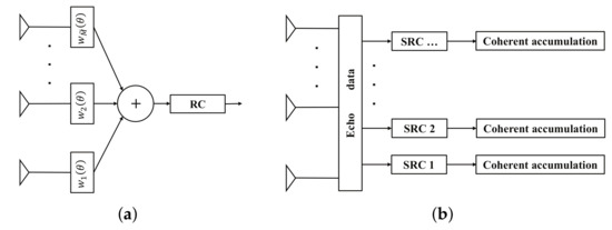
Figure 1. The introduced signal processing scheme. (a) The details of each SRC. (b) The signal processing scheme.

Let us consider a colocated MIMO radar with M transmit antennas, each of which emits a different waveform $x_m\left(l\right)$ with $m=1,2,\cdots ,M$ and $l=1,2,\cdots ,L$, where L denotes the number of discrete time samples of each pulse. Let $\mathbf{x}\left(l\right)={\left[x_1\left(l\right),x_2\left(l\right),\cdots ,x_M\left(l\right)\right]}^{\mathrm{T}}$ be the l-th sample of transmit waveform and $\mathbf{X}=\left[\begin{array}{cccc}\mathbf{x}\left(1\right)& \mathbf{x}\left(2\right)& \cdots & \mathbf{x}\left(L\right)\end{array}\right]$ be the transmit waveform. Then, the AW at the angle $\theta$ is given by:

$$\begin{array}{c}\hfill \begin{array}{c}\hfill \mathbf{s}\left(\theta \right)=vec\left({\mathbf{a}}_t^{\mathrm{T}}\left(\theta \right)\mathbf{X}\right)=\left({\mathbf{I}}_L\otimes {\mathbf{a}}_t^{\mathrm{T}}\left(\theta \right)\right)\overline{\mathbf{x}}\end{array}\end{array}$$

(1)

where $\overline{\mathbf{x}}=vec\left(\mathbf{X}\right)$ and ${\mathbf{a}}_t\left(\theta \right)$ denotes the transmit steering vector. For a uniform linear array (ULA) with half-wavelength separation between two adjacent array antennas, the transmit steering vector is given by:

$$\begin{array}{c}\hfill \begin{array}{c}\hfill {\mathbf{a}}_t\left(\theta \right)={\left[\begin{array}{cccc}1,& e^{-\mathrm{j}\pi sin\left(\theta \right)},& \cdots ,& e^{-\mathrm{j}\left(M-1\right)\pi sin\left(\theta \right)}\end{array}\right]}^{\mathrm{T}}.\end{array}\end{array}$$

(2)

Hence, the power received at angle $\theta$ can be written as:

$$\begin{array}{c}\hfill \begin{array}{c}\hfill P\left(\theta \right)={\mathbf{s}}^{\mathrm{H}}\left(\theta \right)\mathbf{s}\left(\theta \right)={\overline{\mathbf{x}}}^{\mathrm{H}}\mathbf{R}\left(\theta \right)\overline{\mathbf{x}}\end{array}\end{array}$$

(3)

where $\mathbf{R}\left(\theta \right)={\left({\mathbf{I}}_L\otimes {\mathbf{a}}_t^{\mathrm{T}}\left(\theta \right)\right)}^{\mathrm{H}}\left({\mathbf{I}}_L\otimes {\mathbf{a}}_t^{\mathrm{T}}\left(\theta \right)\right)$. $P\left(\theta \right)$ of all the locations under observation is defined as the transmit beampattern, which represents the power distribution in space.

Assume that radar forms J beams at ${\theta }_j,j=1,2,\cdots ,J$ with the transmit power $P\left({\theta }_j\right),j=1,2,\cdots ,J$, respectively, to track the possible targets. Let ${\Omega }_s=\left[-{90}^{\circ },{\theta }_1-W_N^1\right]\cup \left[{\theta }_1+W_N^1,{\theta }_2-W_N^2\right]\cup \cdots \cup \left[{\theta }_{J-1}+W_N^{J-1},{\theta }_J-W_N^J\right]\cup \left[{\theta }_J+W_N^J,{90}^{\circ }\right]$, where $W_N^j,j=1,2,$$\cdots ,J$ denotes half of the natural first null beamwidth of the transmit array. Then, the baseband equivalent of the radar returns at receive antennas is given by:

$$\begin{array}{c}\hfill \begin{array}{c}\hfill \mathbf{Y}=\sum _{j=1}^J{\mathbf{a}}_r\left({\theta }_j\right){\mathbf{s}}^{\mathrm{T}}\left({\theta }_j\right)+\sum _{{\theta }_k\in {\Omega }_s}{\mathbf{a}}_r\left({\theta }_k\right){\mathbf{s}}^{\mathrm{T}}\left({\theta }_k\right)+\mathbf{N}\end{array}\end{array}$$

(4)

where ${\mathbf{a}}_r\left(\theta \right)$ denotes the receive steering vector and $\mathbf{N}\in {\mathbb{C}}^{M\times L}$ is the channel noise with mean zero and variance ${\sigma }^2$. Without loss of generality, in (4), it is assumed that all scatterers have identical complex amplitudes. Similarly, for a ULA with a half-wavelength-spaced antenna,

$$\begin{array}{c}\hfill \begin{array}{c}\hfill {\mathbf{a}}_r\left(\theta \right)={\left[\begin{array}{cccc}1,& e^{-\mathrm{j}\pi sin\left(\theta \right)},& \cdots ,& e^{-\mathrm{j}\left(\tilde{M}-1\right)\pi sin\left(\theta \right)}\end{array}\right]}^{\mathrm{T}}\end{array}\end{array}$$

(5)

where $\tilde{M}$ is the number of receive antennas.

According to the signal processing scheme in Figure 1, the output of receive beamforming for the $\tilde{j}$-th SRC is given by:

$$\begin{array}{c}\hfill \begin{array}{c}\hfill {\mathbf{y}}_{\tilde{j}}={\alpha }_{\tilde{j}\tilde{j}}\mathbf{s}\left({\theta }_{\tilde{j}}\right)+\sum _{j=1,j\ne \tilde{j}}^J{\alpha }_{\tilde{j}j}\mathbf{s}\left({\theta }_j\right)+\sum _{{\theta }_k\in {\Omega }_s}{\alpha }_{\tilde{j}k}\mathbf{s}\left({\theta }_k\right)+{\mathbf{n}}_{\tilde{j}}\end{array}\end{array}$$

(6)

where ${\alpha }_{\tilde{j}j}={\mathbf{w}}^{\mathrm{H}}\left({\theta }_{\tilde{j}}\right){\mathbf{a}}_r\left({\theta }_j\right)$, $\mathbf{w}\left({\theta }_j\right)$ denotes the receive beamformer for the j-th SRC, and ${\mathbf{n}}_j={\mathbf{N}}^{\mathrm{T}}{\mathbf{w}}^{*}\left({\theta }_j\right)$. From (6), it can be seen that the output of receive beamforming is a linear combination of AWs from all directions, and the output power of receive beamforming can be given by:

$$\begin{array}{c}\hfill \begin{array}{c}\hfill E\left[{\mathbf{y}}_{\tilde{j}}^{\mathrm{H}}{\mathbf{y}}_{\tilde{j}}\right]={\left|{\alpha }_{\tilde{j}\tilde{j}}\right|}^{2}P\left({\theta }_{\tilde{j}}\right)+\sum _{j=1,j\ne \tilde{j}}^J{\left|{\alpha }_{\tilde{j}j}\right|}^{2}P\left({\theta }_j\right)+\sum _{{\theta }_k\in {\Omega }_s}{\left|{\alpha }_{\tilde{j}k}\right|}^{2}P\left({\theta }_k\right)+{\sigma }^2{∥\mathbf{w}\left({\theta }_j\right)∥}_2^2.\end{array}\end{array}$$

(7)

Considering the gain of transmit beams and receive beamforming, we have:

$${\left|{\alpha }_{\tilde{j}\tilde{j}}\right|}^2\gg {\left|{\alpha }_{\tilde{j}k}\right|}^2,P\left({\theta }_{\tilde{j}}\right)\gg P\left({\theta }_k\right).$$

(8)

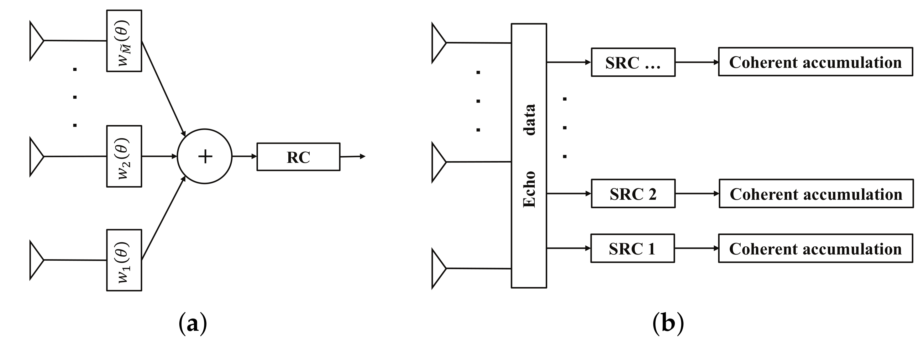
Therefore, the signals from ${\Omega }_s$ can be ignored. We show the suppression of signals from the sidelobes in Figure 2. In this example, a ULA with half-wavelength-spaced antennas is selected, and $M=\tilde{M}=10$. There are two transmit beams at $-{30}^{\circ }$ and $0^{\circ }$, respectively, and the transmit waveform is:

$$\begin{array}{c}\hfill \begin{array}{c}\hfill \mathbf{X}=\frac{\left[{\stackrel{L/\phantom{L2}2}{\overbrace{\begin{array}{ccc}{\mathbf{a}}_t^{*}\left(-{30}^{\circ }\right)& \cdots & {\mathbf{a}}_t^{*}\left(-{30}^{\circ }\right)\end{array}}}}^{}{\stackrel{L/\phantom{L2}2}{\overbrace{\begin{array}{ccc}{\mathbf{a}}_t^{*}\left(0^{\circ }\right)& \cdots & {\mathbf{a}}_t^{*}\left(0^{\circ }\right)\end{array}}}}^{}\right]}{\sqrt{L}}.\end{array}\end{array}$$

(9)

Figure 2. The joint gain of the transmitter and receiver.

For the SRC of direction $-{30}^{\circ }$, the receive beamformer is set as:

$$\begin{array}{c}\hfill \begin{array}{c}\hfill \mathbf{w}\left(-{30}^{\circ }\right)={\mathbf{a}}_r\left(-{30}^{\circ }\right)\end{array}\end{array}$$

(10)

and the input noise is ${\sigma }^2=2$, i.e., the input signal-to-noise-ratio (SNR) is −3 dB.

In Figure 2, we show the transmit beampattern, the output of receive beamforming for $-{30}^{\circ }$, and the output noise level after receive beamforming. It can be seen that the signals from the sidelobes are suppressed below the noise level, and the interference of these signals can be ignored. In fact, for a large number of receive antennas or adaptive receive beamformers, the signals from a beam at $0^{\circ }$ can also be ignored, and we can focus on only the returns from $-{30}^{\circ }$ [12,15]. It can be observed that in Model (4), the interference of the signals within the mainlobe region is neglected. This is because the mainlobe power is mainly concentrated in the signal from the beam-pointing direction, and the signals within the mainlobe region are highly correlated. The detailed proof and results can be found in [22,39].

After the above analysis, the signals from ${\Omega }_s$ are ignored, and the output (6) can be approximated as:

$$\begin{array}{c}\hfill \begin{array}{c}\hfill {\tilde{\mathbf{y}}}_{\tilde{j}}={\alpha }_{\tilde{j}\tilde{j}}\mathbf{s}\left({\theta }_{\tilde{j}}\right)+\sum _{j=1,j\ne \tilde{j}}^J{\alpha }_{\tilde{j}j}\mathbf{s}\left({\theta }_j\right)+{\mathbf{n}}_{\tilde{j}}.\end{array}\end{array}$$

(11)

For the $\tilde{j}$-th SRC, the signal from ${\theta }_{\tilde{j}}$ needs to be extracted. The matched version of the RC for the $\tilde{j}$-th SRC is $\mathbf{s}\left({\theta }_{\tilde{j}}\right)/\phantom{\mathbf{s}\left({\theta }_{\tilde{j}}\right)P\left({\theta }_{\tilde{j}}\right)}P\left({\theta }_{\tilde{j}}\right)$, and the output of the $\tilde{j}$-th SRC is given by:

$$\begin{array}{c}\hfill \begin{array}{c}\hfill {\tilde{y}}_{\tilde{j}}\left(\tau \right)=\frac{{\mathbf{s}}^{\mathrm{H}}\left({\theta }_{\tilde{j}}\right){\mathbf{J}}_{\tau }}{P\left({\theta }_{\tilde{j}}\right)}\left({\alpha }_{\tilde{j}\tilde{j}}\mathbf{s}\left({\theta }_{\tilde{j}}\right)+\sum _{j=1,j\ne \tilde{j}}^J{\alpha }_{\tilde{j}j}\mathbf{s}\left({\theta }_j\right)+{\mathbf{n}}_{\tilde{j}}\right)\\ \hfill ,\tau =-L+1,\cdots ,L-1\end{array}\end{array}$$

(12)

where ${\mathbf{J}}_{\tau }$ is an $L\times L$ shift matrix with the $\left(l_1,l_2\right)$-th element ${\mathbf{J}}_{\tau }\left(l_1,l_2\right)=\delta \left(l_1-l_2-\tau \right)$.

Considering the target velocity is not accurately known, (12) can be extended to [6]:

$$\begin{array}{c}\hfill \begin{array}{c}\hfill \begin{array}{c}\hfill {\tilde{y}}_{\tilde{j}}\left(\tau \right)=\frac{{\mathbf{s}}^{\mathrm{H}}\left({\theta }_{\tilde{j}}\right){\mathbf{J}}_{\tau }}{P\left({\theta }_{\tilde{j}}\right)}\left({\alpha }_{\tilde{j}\tilde{j}}\mathbf{s}\left({\theta }_{\tilde{j}}\right)\odot \mathbf{f}\left({\theta }_{\tilde{j}}\right)+{\displaystyle \sum _{j=1,j\ne \tilde{j}}^J}{\alpha }_{\tilde{j}j}\mathbf{s}\left({\theta }_j\right)\odot \mathbf{f}\left({\theta }_j\right)+{\mathbf{n}}_{\tilde{j}}\right)\\ \hfill ,\tau =-L+1,\cdots ,L-1\end{array}\end{array}\end{array}$$

(13)

where $\mathbf{f}\left({\theta }_j\right)$ denotes the Doppler steering vector of a target at ${\theta }_j$.

From (11) to (13), we can find that the qualities of AWs, such as the AF, PSD, and correlation properties, are important for the radar performance.

3. Problem Formulation

In this section, we formulate the optimization problems of the joint design of the transmit beampattern and AWs.

3.1. Directional Transmit Beampattern Design

Considering a constant transmit power, if the transmit power is sufficiently concentrated in a certain direction, the transmit power allocated to other spatial directions, corresponding to the sidelobe region, will be naturally suppressed. Therefore, the transmit beampattern only needs to approach some key points to ensure the transmit gain and beamwidth. It is assumed that the radar forms J beams at ${\theta }_j,j=1,2,\cdots ,J$. For the ULA with a half-wavelength-spaced antenna, the half of the natural first null beamwidth is about $W_N^j={sin}^{-1}\left(2/\phantom{2Mcos{\theta }_j}Mcos{\theta }_j\right)$. Therefore, in order to control the beamwidth, it is desired that:

$$\begin{array}{c}\hfill \begin{array}{c}\hfill P\left({\theta }_j-W_N^j\right)=P\left({\theta }_j+W_N^j\right)=0,j=1,2,\cdots ,J.\end{array}\end{array}$$

(14)

Next, how to guarantee the transmit gain and concentrate the transmit power in the mainlobe regions is considered. Considering the transmit steering vector in (2) and ${∥\mathbf{X}∥}_{\mathrm{F}}^2=M$, let $v=sin\theta$ denote the normalized direction, and the total transmit power is given by:

$$\begin{array}{c}\hfill \begin{array}{c}\hfill \begin{array}{cc}{\int }_{-1}^{1}P\left(v\right)dv\hfill & ={\overline{\mathbf{x}}}^{\mathrm{H}}\left({\int }_{-1}^1\mathbf{R}\left(v\right)dv\right)\overline{\mathbf{x}}\hfill \\ \hfill & ={\overline{\mathbf{x}}}^{\mathrm{H}}\left({\mathbf{I}}_L\otimes {\int }_{-1}^1{\mathbf{a}}_t^{*}\left(v\right){\mathbf{a}}_t^{\mathrm{T}}\left(v\right)dv\right)\overline{\mathbf{x}}\hfill \\ \hfill & =2M\hfill \end{array}\end{array}\end{array}$$

(15)

where the integral term can be calculated by:

$$\begin{array}{c}\hfill \begin{array}{c}\hfill \mathbf{A}={\int }_{v_l}^{v_u}{\mathbf{a}}_t^{*}\left(v\right){\mathbf{a}}_t^{\mathrm{T}}\left(v\right)dv\end{array}\end{array}$$

(16)

$$\begin{array}{c}\hfill \begin{array}{c}\hfill \mathbf{A}\left(m_1,m_2\right)={\int }_{v_l}^{v_u}{e}^{\mathrm{j}\pi \left(m_1-m_2\right)v}dv\end{array}\end{array}$$

(17)

Suppose that all the transmit power is concentrated in the mainlobe regions, and we have:

$$\begin{array}{c}\hfill \begin{array}{c}\hfill \sum _{j=1}^J{\int }_{v_j-W_{N_v}^j}^{v_j+W_{N_v}^j}P\left(v\right)dv=2M\end{array}\end{array}$$

(18)

$$\begin{array}{c}\hfill \begin{array}{c}\hfill {\int }_{v_j-W_{N_v}^j}^{v_j+W_{N_v}^j}P\left(v\right)dv=2M{\beta }_j\end{array}\end{array}$$

(19)

where $W_{N_v}^j=2/\phantom{2Mcos{\theta }_j}Mcos{\theta }_j$, $v_j=sin{\theta }_j$, and ${\beta }_j$ denote the proportion of the power in the j-th mainlobe region to the total transmit power. It is natural that $\sum _{j=1}^J{\beta }_j=1$.

Let $P_{{\theta }_j}\left(\theta \right)$ represent the transmit beampattern of the following waveform:

$$\begin{array}{c}\hfill \begin{array}{c}\hfill {\mathbf{X}}_{{\theta }_j}=\left[\begin{array}{cccc}{\mathbf{a}}_t^{*}\left({\theta }_j\right)& {\mathbf{a}}_t^{*}\left({\theta }_j\right)& \cdots & {\mathbf{a}}_t^{*}\left({\theta }_j\right)\end{array}\right]/\phantom{\left[\begin{array}{cccc}{\mathbf{a}}_t^{*}\left({\theta }_j\right)& {\mathbf{a}}_t^{*}\left({\theta }_j\right)& \cdots & {\mathbf{a}}_t^{*}\left({\theta }_j\right)\end{array}\right]\sqrt{L}}\sqrt{L}\end{array}\end{array}$$

(20)

and it can be calculated:

$$\begin{array}{c}\hfill \begin{array}{c}\hfill {\eta }_j={\int }_{v_j-W_{N_v}^j}^{v_j+W_{N_v}^j}{P}_{v_j}\left(v\right)dv/\phantom{{\int }_{v_j-W_{N_v}^j}^{v_j+W_{N_v}^j}{P}_{v_j}\left(v\right)dv2M}2M.\end{array}\end{array}$$

(21)

Therefore,

$$\begin{array}{c}\hfill \begin{array}{c}\hfill {\int }_{v_j-W_{N_v}^j}^{v_j+W_{N_v}^j}P\left(v\right)dv=\frac{{\beta }_j}{{\eta }_j}{\int }_{v_j-W_{N_v}^j}^{v_j+W_{N_v}^j}{P}_{v_j}\left(v\right)dv=2M{\beta }_j.\end{array}\end{array}$$

(22)

It can be observed that $P_{{\theta }_j}\left({\theta }_j\right)=M^2$ is the maximum transmit power gain. Hence, it is desired that:

$$\begin{array}{c}\hfill \begin{array}{c}\hfill P\left({\theta }_j\right)=\frac{{\beta }_j}{{\eta }_j}{P}_{{\theta }_j}\left({\theta }_j\right)=\frac{{\beta }_j{M}^2}{{\eta }_j},\end{array}\end{array}$$

(23)

which will guarantee the transmit gain and concentrate the transmit power in the mainlobe regions as much as possible.

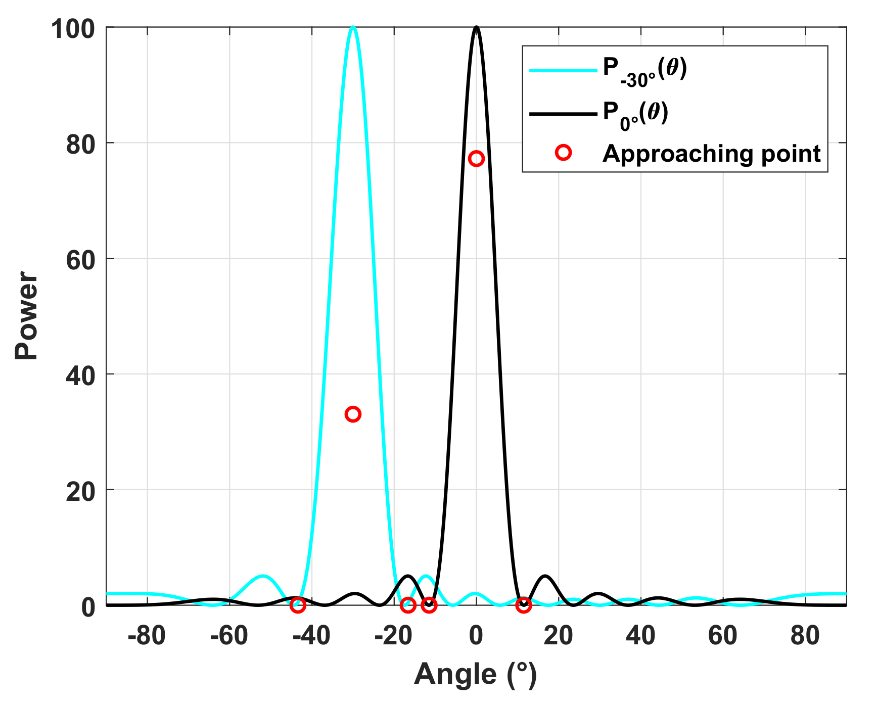
Finally, according to (14) and (23), there are three key points, $\left({\theta }_j-W_N^j,0\right)$, $\left({\theta }_j+W_N^j,0\right)$, and $\left({\theta }_j,{\beta }_j{M}^2/\phantom{{\beta }_j{M}^2{\eta }_j}{\eta }_j\right)$, to approach for each beam in $P\left(\theta \right)$, where the first two points control the beamwidth and the last point guarantees the beam direction and gain. ${\beta }_j$ is a parameter to adjust the power of each beam in $P\left(\theta \right)$, and ${\eta }_j$ ensures that the transmit power is concentrated in the mainlobe regions. In Figure 3, we intuitively show $P_{{\theta }_j}\left(\theta \right)$ and the points that need to be approached in designing the transmit beampattern. In this example, a ULA with half-wavelength-spaced antennas is selected and $M=10$. It is assumed that there are two beams at $-{30}^{\circ }$ and $0^{\circ }$ and $P_{-{30}^{\circ }}\left(\theta \right)$ and $P_{0^{\circ }}\left(\theta \right)$, respectively obtained by (20). ${\beta }_1=0.3$ and ${\beta }_2=0.7$, which means the power ratio of the two beams is $3/377$. According to (21), ${\eta }_1=0.908,{\eta }_2=0.906$ and all the approaching points are obtained.

Figure 3. The representation of approaching points.

3.2. The Joint Design of the Transmit Beampattern and the PSDs of AWs

Let:

$$\begin{array}{c}\hfill \begin{array}{c}\hfill p_j={\beta }_j{M}^2/\phantom{{\beta }_j{M}^2{\eta }_j}{\eta }_j,j=1,2,\cdots ,J\end{array}\end{array}$$

(24)

and it is assumed that:

$$\begin{array}{c}\hfill \begin{array}{c}\hfill P\left({\theta }_j\right)=p_j-{\beta }_j\epsilon ,j=1,2,\cdots ,J\end{array}\end{array}$$

(25)

$$\begin{array}{c}\hfill \begin{array}{c}\hfill P\left({\theta }_j-W_N^j\right)=P\left({\theta }_j+W_N^j\right)={\alpha }_{b}P\left({\theta }_j\right),j=1,2,\cdots ,J\end{array}\end{array}$$

(26)

where ${\beta }_j\epsilon$ denotes the difference between $P\left({\theta }_j\right)$ and $p_j$ and ${\alpha }_b\ll 1$ denotes the gain of $P\left({\theta }_j\pm W_N^j\right)$ relative to $P\left({\theta }_j\right)$. According to the analysis in the previous subsection, it is easy to deduce that $p_j\ge P\left({\theta }_j\right)$, so $\epsilon \ge 0$.

Let $\mathbf{F}\in {\mathbb{C}}^{L\times L}$ denote the discrete Fourier transform (DFT) matrix. According to (1), the spectrum of the AW is:

$$\begin{array}{c}\hfill \begin{array}{c}\hfill {\mathbf{s}}_f\left(\theta \right)=\mathbf{F}\left({\mathbf{I}}_L\otimes {\mathbf{a}}_t^{\mathrm{T}}\left(\theta \right)\right)\overline{\mathbf{x}}\end{array}\end{array}$$

(27)

and the PSD of the AW is:

$$\begin{array}{c}\hfill \begin{array}{c}\hfill \begin{array}{cc}{s}_f\left(\theta ,l\right)\hfill & ={\mathbf{s}}_f^{\mathrm{H}}\left(\theta \right){\mathbf{E}}_l{\mathbf{s}}_f\left(\theta \right)\hfill \\ \hfill & ={\overline{\mathbf{x}}}^{\mathrm{H}}{\left({\mathbf{I}}_L\otimes {\mathbf{a}}_t^{\mathrm{T}}\left(\theta \right)\right)}^{\mathrm{H}}{\mathbf{F}}^{\mathrm{H}}{\mathbf{E}}_l\mathbf{F}\left({\mathbf{I}}_L\otimes {\mathbf{a}}_t^{\mathrm{T}}\left(\theta \right)\right)\overline{\mathbf{x}}\hfill \\ \hfill & ={\overline{\mathbf{x}}}^{\mathrm{H}}\mathbf{B}\left(\theta ,l\right)\overline{\mathbf{x}},l=1,2,\cdots ,L\hfill \end{array}\end{array}\end{array}$$

(28)

where $\mathbf{B}\left(\theta ,l\right)={\left({\mathbf{I}}_L\otimes {\mathbf{a}}_t^{\mathrm{T}}\left(\theta \right)\right)}^{\mathrm{H}}{\mathbf{F}}^{\mathrm{H}}{\mathbf{E}}_l\mathbf{F}\left({\mathbf{I}}_L\otimes {\mathbf{a}}_t^{\mathrm{T}}\left(\theta \right)\right)$ and ${\mathbf{E}}_l$ is an $L\times L$ matrix whose $\left(l,l\right)$-th element is 1, and 0 otherwise. If ${\mathbf{F}}^{\mathrm{H}}\mathbf{F}={\mathbf{I}}_L$, it is easy to deduce that:

$$\begin{array}{c}\hfill \begin{array}{c}\hfill P\left(\theta \right)={\mathbf{s}}_f^{\mathrm{H}}\left(\theta \right){\mathbf{s}}_f\left(\theta \right)=\sum _{l=1}^L{s}_f\left(\theta ,l\right)\end{array}\end{array}$$

(29)

Let $d\left({\theta }_j,l\right),l=1,2,\cdots L$ denote the desired PSD for $\mathbf{s}\left({\theta }_j\right)$. According to (29), we have:

$$\begin{array}{c}\hfill \begin{array}{c}\hfill P\left({\theta }_j\right)=\sum _{l=1}^L{s}_f\left({\theta }_j,l\right),j=1,2,\cdots ,J\end{array}\end{array}$$

(30)

$$\begin{array}{c}\hfill \begin{array}{c}\hfill p_j=\sum _{l=1}^{L}d\left({\theta }_j,l\right),j=1,2,\cdots ,J.\end{array}\end{array}$$

(31)

If:

$$\begin{array}{c}\hfill \begin{array}{c}\hfill {\overline{s}}_f\left({\theta }_j,l\right)=P\left({\theta }_j\right)/\phantom{P\left({\theta }_j\right)L}L,l=1,2,\cdots ,L,j=1,2,\cdots ,J\end{array}\end{array}$$

(32)

$$\begin{array}{c}\hfill \begin{array}{c}\hfill \overline{d}\left({\theta }_j,l\right)=p_j/\phantom{p_{j}L}L,l=1,2,\cdots ,L,j=1,2,\cdots ,J\end{array}\end{array}$$

(33)

then we have:

$$\begin{array}{c}\hfill \begin{array}{c}\hfill L\left(\overline{d}\left({\theta }_j,l\right)-{\overline{s}}_f\left({\theta }_j,l\right)\right)={\beta }_j\epsilon ,l=1,2,\cdots ,L,j=1,2,\cdots ,J\end{array}\end{array}$$

(34)

Therefore, in order to approach the desired PSD, we let:

$$\begin{array}{c}\hfill \begin{array}{c}\hfill L\left|s_f\left({\theta }_j,l\right)-d\left({\theta }_j,l\right)\right|\le {\beta }_j\epsilon ,l=1,2,\cdots ,L,j=1,2,\cdots ,J.\end{array}\end{array}$$

(35)

and the above constraint can be equivalently converted to:

$$\begin{array}{c}\hfill \begin{array}{c}\hfill \begin{array}{c}L\left(s_f\left({\theta }_j,l\right)-d\left({\theta }_j,l\right)\right)\le {\beta }_j\epsilon ,l=1,2,\cdots ,L,j=1,2,\cdots ,J\hfill \\ L\left(d\left({\theta }_j,l\right)-s_f\left({\theta }_j,l\right)\right)\le {\beta }_j\epsilon ,l=1,2,\cdots ,L,j=1,2,\cdots ,J\hfill \end{array}.\end{array}\end{array}$$

(36)

Let:

$$\begin{array}{c}\hfill \begin{array}{c}\hfill w_{lj}=\left|s_f\left({\theta }_j,l\right)-d\left({\theta }_j,l\right)\right|,l=1,2,\cdots ,L,j=1,2,\cdots ,J.\end{array}\end{array}$$

(37)

The constraint (35) means more attention is paid to the large $w_{lj}$, and otherwise, less attention is paid. This behavior is similar to the least squares method [40].

Summarizing, the joint design of the transmit beampattern and the PSDs of AWs can be formulated as the following constrained optimization problem:

$$\begin{array}{c}\hfill \begin{array}{c}\hfill \begin{array}{c}\underset{\overline{\mathbf{x}},\epsilon }{min}\epsilon \hfill \\ s.t.p_j-P\left({\theta }_j\right)\le {\beta }_j\epsilon ,j=1,2,\cdots ,J\hfill \\ P\left({\theta }_j-W_N^j\right)\le {\alpha }_b\left(p_j-{\beta }_j\epsilon \right),j=1,2,\cdots ,J\hfill \\ P\left({\theta }_j+W_N^j\right)\le {\alpha }_b\left(p_j-{\beta }_j\epsilon \right),j=1,2,\cdots ,J\hfill \\ L\left(s_f\left({\theta }_j,l\right)-d\left({\theta }_j,l\right)\right)\le {\beta }_j\epsilon ,\hfill \\ l=1,2,\cdots ,L,j=1,2,\cdots ,J\hfill \\ L\left(d\left({\theta }_j,l\right)-s_f\left({\theta }_j,l\right)\right)\le {\beta }_j\epsilon ,\hfill \\ l=1,2,\cdots ,L,j=1,2,\cdots ,J\hfill \\ \epsilon \ge 0,\left|\overline{\mathbf{x}}\right|=\frac{{\mathbf{1}}_{ML}}{\sqrt{L}}\hfill \end{array}\end{array}\end{array}$$

(38)

where the first three constraints are to approximate the key points in the beampattern and the last constraint enforces the waveform to be the CM.

3.3. Joint Design of the Transmit Beampattern and the Spectral Compatibility and Similarity of AWs

For the transmit beampattern, the setting in (24)∼(26) is still used in this subsection. Let ${\Omega }_j$ denote the occupied frequency band at ${\theta }_j$. According to (30), the spectral compatibility constraint can be represented as:

$$\begin{array}{c}\hfill \begin{array}{c}\hfill \sum _{l\in {\Omega }_j}{s}_f\left({\theta }_j,l\right)\le {\alpha }_{f}P\left({\theta }_j\right),j=1,2,\cdots ,J\end{array}\end{array}$$

(39)

where ${\alpha }_f<1$ denotes the ratio of the unavailable band power to the total power at ${\theta }_j$.

Let $\mathbf{r}\left({\theta }_j\right)$ denote the spectrum of the reference waveform for $\mathbf{s}\left({\theta }_j\right)$. Here, considering the spectral compatibility constraint, in order to guarantee the feasibility of the problem, the similarity is expressed in the frequency domain as follows:

$$\begin{array}{c}\hfill \begin{array}{c}\hfill {∥{\mathbf{s}}_f\left({\theta }_j\right)-\mathbf{r}\left({\theta }_j\right)∥}_2^2,j=1,2,\cdots ,J.\end{array}\end{array}$$

(40)

According to (29), we have:

$$\begin{array}{c}\hfill \begin{array}{c}\hfill {∥{\mathbf{s}}_f\left({\theta }_j\right)∥}_2^2=P\left({\theta }_j\right),j=1,2,\cdots ,J\end{array}\end{array}$$

(41)

$$\begin{array}{c}\hfill \begin{array}{c}\hfill {∥\mathbf{r}\left({\theta }_j\right)∥}_2^2=p_j,j=1,2,\cdots ,J.\end{array}\end{array}$$

(42)

Therefore,

$$\begin{array}{c}\hfill \begin{array}{c}\hfill {∥{\mathbf{s}}_f\left({\theta }_j\right)-\mathbf{r}\left({\theta }_j\right)∥}_2^2\le 4p_j,j=1,2,\cdots ,J\end{array}\end{array}$$

(43)

$$\begin{array}{c}\hfill \begin{array}{c}\hfill {∥{\mathbf{s}}_f\left({\theta }_j\right)-\mathbf{r}\left({\theta }_j\right)∥}_2^2\ge {\left(\sqrt{p_j-{\beta }_j\epsilon }-\sqrt{p_j}\right)}^2,j=1,2,\cdots ,J.\end{array}\end{array}$$

(44)

According to the Cauchy inequality,

$$\begin{array}{c}\hfill \begin{array}{c}\hfill 0\le {\left(\sqrt{p_j-{\beta }_j\epsilon }-\sqrt{p_j}\right)}^2\le {\beta }_j\epsilon .\end{array}\end{array}$$

(45)

Hence, the similarity constraint is set as:

$$\begin{array}{c}\hfill \begin{array}{c}\hfill {∥{\mathbf{s}}_f\left({\theta }_j\right)-\mathbf{r}\left({\theta }_j\right)∥}_2^2\le {\alpha }_s{\beta }_j\epsilon ,j=1,2,\cdots ,J\end{array}\end{array}$$

(46)

where ${\alpha }_s\ge 1$ is a parameter ruling the extent of the similarity.

Summarizing, the following cost function is proposed to jointly design the transmit beampattern and the AWs with spectral compatibility and similarity:

$$\begin{array}{c}\hfill \begin{array}{c}\hfill \begin{array}{c}\underset{\overline{\mathbf{x}},\epsilon }{min}\epsilon \hfill \\ s.t.p_j-P\left({\theta }_j\right)\le {\beta }_j\epsilon ,j=1,2,\cdots ,J\hfill \\ P\left({\theta }_j-W_N^j\right)\le {\alpha }_b\left(p_j-{\beta }_j\epsilon \right),j=1,2,\cdots ,J\hfill \\ P\left({\theta }_j+W_N^j\right)\le {\alpha }_b\left(p_j-{\beta }_j\epsilon \right),j=1,2,\cdots ,J\hfill \\ {∥{\mathbf{s}}_f\left({\theta }_j\right)-\mathbf{r}\left({\theta }_j\right)∥}_2^2\le {\alpha }_s{\beta }_j\epsilon ,j=1,2,\cdots ,J\hfill \\ {\displaystyle \sum _{l\in {\Omega }_j}}{s}_f\left({\theta }_j,l\right)\le {\alpha }_f\left(p_j-{\beta }_j\epsilon \right),j=1,2,\cdots ,J\hfill \\ \epsilon \ge 0,\left|\overline{\mathbf{x}}\right|=\frac{{\mathbf{1}}_{ML}}{\sqrt{L}}\hfill \end{array}\end{array}\end{array}$$

(47)

4. Waveform Optimization Algorithm for the Joint Design

In this section, the proposed problems (38) and (47) are unified into the same framework, and an algorithm based on the ADMM and modified L-BFGS is proposed to solve the problem.

4.1. Proposed Algorithm

Problems (38) and (47) can be recast as:

$$\begin{array}{c}\hfill \begin{array}{c}\hfill \begin{array}{c}\underset{\mathbf{\phi },\mathbf{z}}{min}{\mathbf{\lambda }}^{\mathrm{T}}\mathbf{z}\hfill \\ s.t.\mathbf{\eta }+\mathbf{Kz}=\mathbf{0}\hfill \\ \mathbf{z}\ge \mathbf{0}\hfill \end{array}\end{array}\end{array}$$

(48)

where $\overline{\mathbf{x}}=exp\left(\mathrm{j}\mathbf{\phi }\right)/\phantom{exp\left(\mathrm{j}\phi \right)\sqrt{L}}\sqrt{L}$, the $exp\left(·\right)$ operation is imposed in an elementwise way, and:

$$\begin{array}{c}\hfill \begin{array}{c}\hfill \mathbf{\lambda }={\left[\begin{array}{cccc}0,& 0,& \cdots ,& 1\end{array}\right]}^{\mathrm{T}}\end{array}\end{array}$$

(49)

$$\begin{array}{c}\hfill \begin{array}{c}\hfill \mathbf{K}=\left[\begin{array}{cc}\mathbf{I},& -\mathbf{\kappa }\end{array}\right]\end{array}\end{array}$$

(50)

Let:

$$\begin{array}{c}\hfill \begin{array}{c}\hfill {\mathbf{\eta }}_1=\left[\begin{array}{cccc}{p}_1-P\left({\theta }_1\right),& p_2-P\left({\theta }_2\right),& \cdots ,& p_J-P\left({\theta }_J\right)\end{array}\right]\end{array}\end{array}$$

(51)

$$\begin{array}{c}\hfill \begin{array}{c}\hfill {\mathbf{\eta }}_2=\left[\begin{array}{cccc}P\left({\theta }_1-W_N^1\right)-{\alpha }_b{p}_1,& P\left({\theta }_2-W_N^2\right)-{\alpha }_b{p}_2,& \cdots ,& P\left({\theta }_J-W_N^J\right)-{\alpha }_b{p}_J\end{array}\right]\end{array}\end{array}$$

(52)

$$\begin{array}{c}\hfill \begin{array}{c}\hfill {\mathbf{\eta }}_3=\left[\begin{array}{cccc}P\left({\theta }_1+W_N^1\right)-{\alpha }_b{p}_1,& P\left({\theta }_2+W_N^2\right)-{\alpha }_b{p}_2,& \cdots ,& P\left({\theta }_J+W_N^J\right)-{\alpha }_b{p}_J\end{array}\right]\end{array}\end{array}$$

(53)

$$\begin{array}{c}\hfill \begin{array}{c}\hfill {\mathbf{\eta }}_4=\left[\begin{array}{cccc}L\left(s_f\left({\theta }_1,1\right)-d\left({\theta }_1,1\right)\right),& L\left(s_f\left({\theta }_1,2\right)-d\left({\theta }_1,2\right)\right),& \cdots ,& L\left(s_f\left({\theta }_J,L\right)-d\left({\theta }_J,L\right)\right)\end{array}\right]\end{array}\end{array}$$

(54)

$$\begin{array}{c}\hfill \begin{array}{c}\hfill {\mathbf{\eta }}_5=\left[\begin{array}{cccc}L\left(d\left({\theta }_1,1\right)-s_f\left({\theta }_1,1\right)\right),& L\left(d\left({\theta }_1,2\right)-s_f\left({\theta }_1,2\right)\right),& \cdots ,& L\left(d\left({\theta }_J,L\right)-s_f\left({\theta }_J,L\right)\right)\end{array}\right]\end{array}\end{array}$$

(55)

$$\begin{array}{c}\hfill \begin{array}{c}\hfill {\mathbf{\eta }}_6=\left[\begin{array}{cccc}{∥{\mathbf{s}}_f\left({\theta }_1\right)-\mathbf{r}\left({\theta }_1\right)∥}_2^2,& {∥{\mathbf{s}}_f\left({\theta }_2\right)-\mathbf{r}\left({\theta }_2\right)∥}_2^2,& \cdots ,& {∥{\mathbf{s}}_f\left({\theta }_J\right)-\mathbf{r}\left({\theta }_J\right)∥}_2^2\end{array}\right]\end{array}\end{array}$$

(56)

$$\begin{array}{c}\hfill \begin{array}{c}\hfill {\mathbf{\eta }}_7=\left[\begin{array}{cccc}{\displaystyle \sum _{l\in {\Omega }_1}}{s}_f\left({\theta }_1,l\right)-{\alpha }_f{p}_1,& {\displaystyle \sum _{l\in {\Omega }_2}}{s}_f\left({\theta }_2,l\right)-{\alpha }_f{p}_2,& \cdots ,& {\displaystyle \sum _{l\in {\Omega }_J}}{s}_f\left({\theta }_J,l\right)-{\alpha }_f{p}_J\end{array}\right]\end{array}\end{array}$$

(57)

$$\begin{array}{c}\hfill \begin{array}{c}\hfill {\mathbf{\kappa }}_1=\left[\begin{array}{cccc}{\beta }_1,& {\beta }_2,& \cdots ,& {\beta }_J\end{array}\right]\end{array}\end{array}$$

(58)

$$\begin{array}{c}\hfill \begin{array}{c}\hfill {\mathbf{\kappa }}_2=\left[\begin{array}{cccc}{\beta }_1{\mathbf{1}}_{1\times L},& {\beta }_2{\mathbf{1}}_{1\times L},& \cdots ,& {\beta }_J{\mathbf{1}}_{1\times L}\end{array}\right].\end{array}\end{array}$$

(59)

For Problem (38),

$$\begin{array}{c}\hfill \begin{array}{c}\hfill \mathbf{\eta }={\left[{\mathbf{\eta }}_1,{\mathbf{\eta }}_2,{\mathbf{\eta }}_3,{\mathbf{\eta }}_4,{\mathbf{\eta }}_5\right]}^{\mathrm{T}}\end{array}\end{array}$$

(60)

$$\begin{array}{c}\hfill \begin{array}{c}\hfill \mathbf{\kappa }={\left[{\mathbf{\kappa }}_1,-{\alpha }_b{\mathbf{\kappa }}_1,-{\alpha }_b{\mathbf{\kappa }}_1,{\mathbf{\kappa }}_2,{\mathbf{\kappa }}_2\right]}^{\mathrm{T}}\end{array}\end{array}$$

(61)

$$\begin{array}{c}\hfill \begin{array}{c}\hfill \mathbf{K}\in {\mathbb{R}}^{\left(3J+2JL\right)\times \left(3J+2JL+1\right)}\end{array}\end{array}$$

(62)

For Problem (47),

$$\begin{array}{c}\hfill \begin{array}{c}\hfill \mathbf{\eta }={\left[{\mathbf{\eta }}_1,{\mathbf{\eta }}_2,{\mathbf{\eta }}_3,{\mathbf{\eta }}_6,{\mathbf{\eta }}_7\right]}^{\mathrm{T}}\end{array}\end{array}$$

(63)

$$\begin{array}{c}\hfill \begin{array}{c}\hfill \mathbf{\kappa }={\left[{\mathbf{\kappa }}_1,-{\alpha }_b{\mathbf{\kappa }}_1,-{\alpha }_b{\mathbf{\kappa }}_1,{\alpha }_s{\mathbf{\kappa }}_1,-{\alpha }_f{\mathbf{\kappa }}_1\right]}^{\mathrm{T}}\end{array}\end{array}$$

(64)

$$\begin{array}{c}\hfill \begin{array}{c}\hfill \mathbf{K}\in {\mathbb{R}}^{5J\times \left(5J+1\right)}\end{array}\end{array}$$

(65)

The augmented Lagrangian function of Problem (48) can be written as:

$$\begin{array}{c}\hfill \begin{array}{c}\hfill \mathcal{L}\left(\mathbf{\phi },\mathbf{z},\mathbf{u}\right)={\mathbf{\lambda }}^{\mathrm{T}}\mathbf{z}+{\mathbf{u}}^{\mathrm{T}}\left(\mathbf{\eta }+\mathbf{Kz}\right)+\frac{\rho }{2}{∥\mathbf{\eta }+\mathbf{Kz}∥}^2\end{array}\end{array}$$

(66)

where $\mathbf{u}$ is the Lagrange multiplier associated with the equality constraint and $\rho >0$ is a penalty parameter.

Under the ADMM framework, the proposed algorithm can be described as:

$$\begin{array}{c}\hfill \begin{array}{c}\hfill {\mathbf{\phi }}^{\left(\ell +1\right)}=arg\underset{\mathbf{\phi }}{min}\mathcal{L}\left(\mathbf{\phi },{\mathbf{z}}^{\left(\ell \right)},{\mathbf{u}}^{\left(\ell \right)}\right)\end{array}\end{array}$$

(67)

$$\begin{array}{c}\hfill \begin{array}{c}\hfill {\mathbf{z}}^{\left(\ell +1\right)}=arg\underset{\mathbf{z}\ge \mathbf{0}}{min}\mathcal{L}\left({\mathbf{\phi }}^{\left(\ell +1\right)},\mathbf{z},{\mathbf{u}}^{\left(\ell \right)}\right)\end{array}\end{array}$$

(68)

$$\begin{array}{c}\hfill \begin{array}{c}\hfill {\mathbf{u}}^{\left(\ell +1\right)}={\mathbf{u}}^{\left(\ell \right)}+\rho \left({\mathbf{\eta }}^{\left(\ell +1\right)}+\mathbf{K}{\mathbf{z}}^{\left(\ell +1\right)}\right)\end{array}\end{array}$$

(69)

where ℓ is the iteration number.

In what follows, the solutions to the alternating minimization problems from (67) to (68) are presented:

(1)

Update $\mathbf{\phi }$:

It is noted that $\mathcal{L}\left(\mathbf{\phi },{\mathbf{z}}^{\left(\ell \right)},{\mathbf{u}}^{\left(\ell \right)}\right)$ is a nonconvex quartic function with respect to $\mathbf{\phi }$. Therefore, it is difficult to obtain the minimizers of $\mathcal{L}\left(\mathbf{\phi },{\mathbf{z}}^{\left(\ell \right)},{\mathbf{u}}^{\left(\ell \right)}\right)$ directly. However, the unconstrained formulation renders the problem amenable to the use of L-BFGS-type iterative procedures, which can be efficiently implemented. Moreover, the work [38] showed that the modified L-BFGS possesses global convergence for the nonconvex problem. The gradient of $\mathcal{L}\left(\mathbf{\phi },{\mathbf{z}}^{\left(\ell \right)},{\mathbf{u}}^{\left(\ell \right)}\right)$ is:

$$\begin{array}{c}\hfill \begin{array}{c}\hfill {\nabla }_{\mathbf{\phi }}\mathcal{L}\left(\mathbf{\phi },{\mathbf{z}}^{\left(\ell \right)},{\mathbf{u}}^{\left(\ell \right)}\right)={\Pi }^{\mathrm{T}}{\mathbf{u}}^{\left(\ell \right)}+\rho {\Pi }^{\mathrm{T}}\left(\mathbf{\eta }+\mathbf{K}{\mathbf{z}}^{\left(\ell \right)}\right)\end{array}\end{array}$$

(70)

where $\Pi ={\partial \mathbf{\eta }/\phantom{\partial \mathbf{\eta }\partial \mathbf{\phi }}\partial \mathbf{\phi }}^{\mathrm{T}}$. See Appendix A for the detailed calculation of $\Pi$. With the gradient, the modified L-BFGS can be implemented;

(2)

Update $\mathbf{z}$:

It can be noticed that $\mathcal{L}\left({\mathbf{\phi }}^{\left(\ell +1\right)},\mathbf{z},{\mathbf{u}}^{\left(\ell \right)}\right)$ is a convex quadratic function with respect to $\mathbf{z}$. Then, by setting the gradient of $\mathcal{L}\left({\mathbf{\phi }}^{\left(\ell +1\right)},\mathbf{z},{\mathbf{u}}^{\left(\ell \right)}\right)$ to be zero, the global minimizer of $\mathcal{L}\left({\mathbf{\phi }}^{\left(\ell +1\right)},\mathbf{z},{\mathbf{u}}^{\left(\ell \right)}\right)$ can be obtained:

$$\begin{array}{c}\hfill \begin{array}{c}\hfill {\mathbf{z}}_{opt}=-\frac{{\left({\mathbf{K}}^{\mathrm{T}}\mathbf{K}\right)}^{†}\left(\mathbf{\lambda }+{\mathbf{K}}^{\mathrm{T}}{\mathbf{u}}^{\left(\ell \right)}+\rho {\mathbf{K}}^{\mathrm{T}}{\mathbf{\eta }}^{\left(\ell +1\right)}\right)}{\rho }\end{array}\end{array}$$

(71)

where ${\left(·\right)}^{†}$ denotes the Moore–Penrose pseudoinverse matrix.

By projecting ${\mathbf{z}}_{opt}$ onto the feasible region, we have:

$$\begin{array}{c}\hfill \begin{array}{c}\hfill {\mathbf{z}}^{\left(\ell +1\right)}=\underset{\left[0,+\infty \right)}{\mathcal{P}}\left({\mathbf{z}}_{opt}\right)\end{array}\end{array}$$

(72)

where $\mathcal{P}\left(·\right)$ is imposed in an elementwise way.

According to the above analysis, we summarize the proposed algorithm in Algorithm 1.

Algorithm 1: Waveform optimization algorithm for the joint design.

Require:  The initial variables ${\mathbf{\phi }}^{\left(1\right)},{\mathbf{z}}^{\left(1\right)},{\mathbf{u}}^{\left(1\right)}$, $\ell =1$ and the penalty parameter $\rho >0$. Ensure:  $\overline{\mathbf{x}}=exp\left(\mathrm{j}{\mathbf{\phi }}^{\left(\ell +1\right)}\right)/\phantom{exp\left(\mathrm{j}{\mathbf{\phi }}^{\left(\ell +1\right)}\right)\sqrt{L}}\sqrt{L}$ 1: repeat 2:     Compute ${\mathbf{\phi }}^{\left(\ell +1\right)}$ using the modified L-BFGS method. 3:     Compute ${\mathbf{z}}^{\left(\ell +1\right)}$ via (72). 4:     Update ${\mathbf{u}}^{\left(\ell +1\right)}$ via (69). 5:     Set $\ell =\ell +1$. 6: until some termination conditions are satisfied.

4.2. Algorithm Convergence

In this subsection, the convergence of the proposed algorithm is analyzed. The following assumptions [37,38] are needed for this purpose.

Assumption 1.

The function $\mathcal{L}\left(\mathbf{\phi },{\mathbf{z}}^{\left(\ell \right)},{\mathbf{u}}^{\left(\ell \right)}\right)$ satisfies the Lipschitz continuous condition, i.e., there exists a constant $\mathcal{K}>0$ such that:

$$\begin{array}{c}\hfill \begin{array}{c}\hfill {∥{\nabla }_{\mathbf{\phi }}\mathcal{L}\left(\mathbf{\phi },{\mathbf{z}}^{\left(\ell \right)},{\mathbf{u}}^{\left(\ell \right)}\right)-{\nabla }_{\mathbf{\phi }}\mathcal{L}\left(\tilde{\mathbf{\phi }},{\mathbf{z}}^{\left(\ell \right)},{\mathbf{u}}^{\left(\ell \right)}\right)∥}_2\le \mathcal{K}{∥\mathbf{\phi }-\tilde{\mathbf{\phi }}∥}_2\end{array}\end{array}$$

(73)

Assumption 2.

The augmented Lagrangian function ${\mathcal{L}}_0\left(\mathbf{\phi },\mathbf{z},\mathbf{u}\right)$, where:

$$\begin{array}{c}\hfill \begin{array}{c}\hfill {\mathcal{L}}_0\left(\mathbf{\phi },\mathbf{z},\mathbf{u}\right)={\mathbf{\lambda }}^{\mathrm{T}}\mathbf{z}+{\mathbf{u}}^{\mathrm{T}}\left(\mathbf{\eta }+\mathbf{Kz}\right)\end{array}\end{array}$$

(74)

has a saddle point $\left({\mathbf{\phi }}_s,{\mathbf{z}}_s,{\mathbf{u}}_s\right)$.

Theorem 1.

Under Assumptions 1 and 2, the proposed algorithm iterates satisfy the following:

(1)

${\mathbf{c}}^{\left(\ell \right)}\to 0$ as $\ell \to \infty$, where $\mathbf{c}=\mathbf{\eta }+\mathbf{Kz}$. This means that the iterates approach feasibility;

(2)

${\epsilon }^{\left(\ell \right)}\to {\epsilon }_s$ as $\ell \to \infty$, where $\epsilon ={\mathbf{\lambda }}^{\mathrm{T}}\mathbf{z}$.

Proof. 

See Appendix A. □

4.3. Reduce the Computational Complexity

As seen from Algorithm 1, the main computational cost of the proposed algorithm is dominated by $\mathbf{\eta }$ and ${\nabla }_{\mathbf{\phi }}\mathcal{L}\left(\mathbf{\phi },{\mathbf{z}}^{\left(\ell \right)},{\mathbf{u}}^{\left(\ell \right)}\right)$. For $\mathbf{\eta }$, the calculation mainly includes $P\left(\theta \right)$ and $s_f\left(\theta ,l\right)$. If $P\left(\theta \right)$ is calculated by (3) directly, the matrix $\mathbf{R}\left(\theta \right)$ occupies a large memory space, and the computational complexity is high. Therefore, a more efficient way is to calculate $\mathbf{s}\left(\theta \right)$ first and then calculate $P\left(\theta \right)$. In this way, the memory consumption is small, and the computational complexity is about $O\left(2ML+L\right)$. For the calculation of $s_f\left(\theta ,l\right)$, we can calculate $\mathbf{s}\left(\theta \right)$ first and obtain $s_f\left(\theta ,l\right)$ by fast Fourier transform (FFT). Summarizing, the computational complexity of obtaining $s_f\left(\theta ,l\right),l=1,2,\cdots ,L$ is about $O\left(ML+LlogL\right)$.

According to (70), the calculation of ${\nabla }_{\mathbf{\phi }}\mathcal{L}\left(\mathbf{\phi },{\mathbf{z}}^{\left(\ell \right)},{\mathbf{u}}^{\left(\ell \right)}\right)$ mainly includes $\mathbf{\eta }$ and $\Pi$. From Appendix A, the common items for calculating $\mathbf{\eta }$ and $\Pi$ are $\mathbf{R}\left(\theta \right)\overline{\mathbf{x}}$ and $\mathbf{B}\left(\theta ,l\right)\overline{\mathbf{x}}$. $\mathbf{R}\left(\theta \right)\overline{\mathbf{x}}$ can then be rewritten as:

$$\begin{array}{c}\hfill \begin{array}{c}\hfill \mathbf{R}\left(\theta \right)\overline{\mathbf{x}}=vec\left({\mathbf{a}}_t^{*}\left(\theta \right){\mathbf{s}}^{\mathrm{T}}\left(\theta \right)\right).\end{array}\end{array}$$

(75)

Therefore, the calculation cost of $\mathbf{R}\left(\theta \right)\overline{\mathbf{x}}$ is about $O\left(2ML\right)$. For $\mathbf{B}\left(\theta ,l\right)\overline{\mathbf{x}},l=1,2,\cdots ,L$, it can be obtained by:

$$\begin{array}{c}\hfill \begin{array}{c}\hfill {\mathbf{A}}_f\left(\theta \right)diag\left({\mathbf{s}}_f\left(\theta \right)\right)\end{array}\end{array}$$

(76)

where ${\mathbf{A}}_f\left(\theta \right)={\left(\mathbf{F}\left({\mathbf{I}}_L\otimes {\mathbf{a}}_t^{\mathrm{T}}\left(\theta \right)\right)\right)}^{\mathrm{H}}$. Therefore, the computational complexity of obtaining $\mathbf{B}\left(\theta ,l\right)\overline{\mathbf{x}},l=1,2,\cdots ,L$ is about $O\left(M{L}^2+LlogL\right)$.

5. Simulation Results

In this section, we show the simulation results of the proposed problems (38) and (47) successively. In addition, the application of Problem (47) in AWs’ orthogonality design is also shown. Unless otherwise specified, in all the simulations, we considered a ULA with $M=10$ transmit antennas separated by a half-wavelength.

For Problem (38), the residuals of the proposed algorithm in the ℓ-th iteration are defined as ${∥{\mathbf{c}}^{\left(\ell \right)}∥}_2/\phantom{{∥{\mathbf{c}}^{\left(\ell \right)}∥}_2\left(3J+2JL\right)}\left(3J+2JL\right)$ and $\left|{\epsilon }^{\left(\ell \right)}-{\epsilon }^{\left(\ell -1\right)}\right|$. For Problem (47), the residuals of the proposed algorithm in the ℓ-th iteration are defined as ${∥{\mathbf{c}}^{\left(\ell \right)}∥}_2/\phantom{{∥{\mathbf{c}}^{\left(\ell \right)}∥}_{2}5J}5J$ and $\left|{\epsilon }^{\left(\ell \right)}-{\epsilon }^{\left(\ell -1\right)}\right|$. The termination condition is set as both of the residuals are less than ${10}^{-4}$. Unless otherwise specified, in all the simulations, the penalty parameter $\rho =10$. All the simulations were performed in the MATLAB 2017b/Windows 7 environment on a computer with a 3.2 GHz CPU and 8 GB RAM.

5.1. The Joint Design of the Transmit Beampattern and the PSDs of AWs

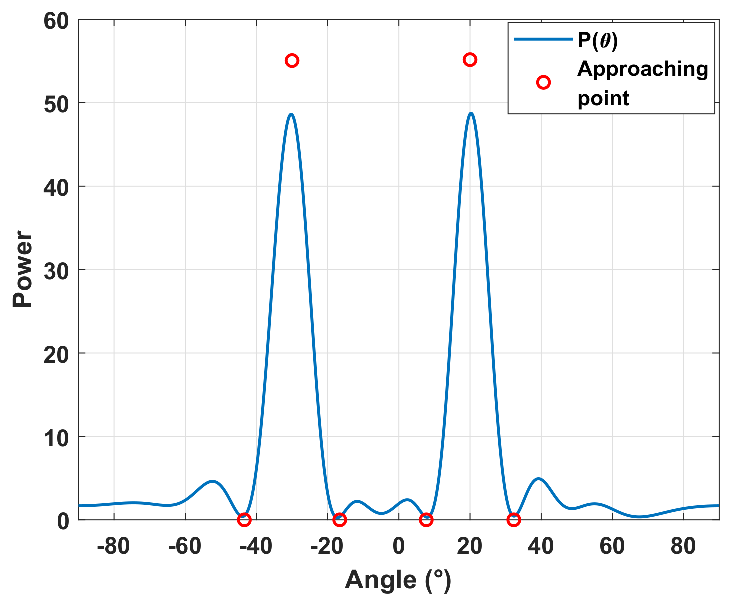
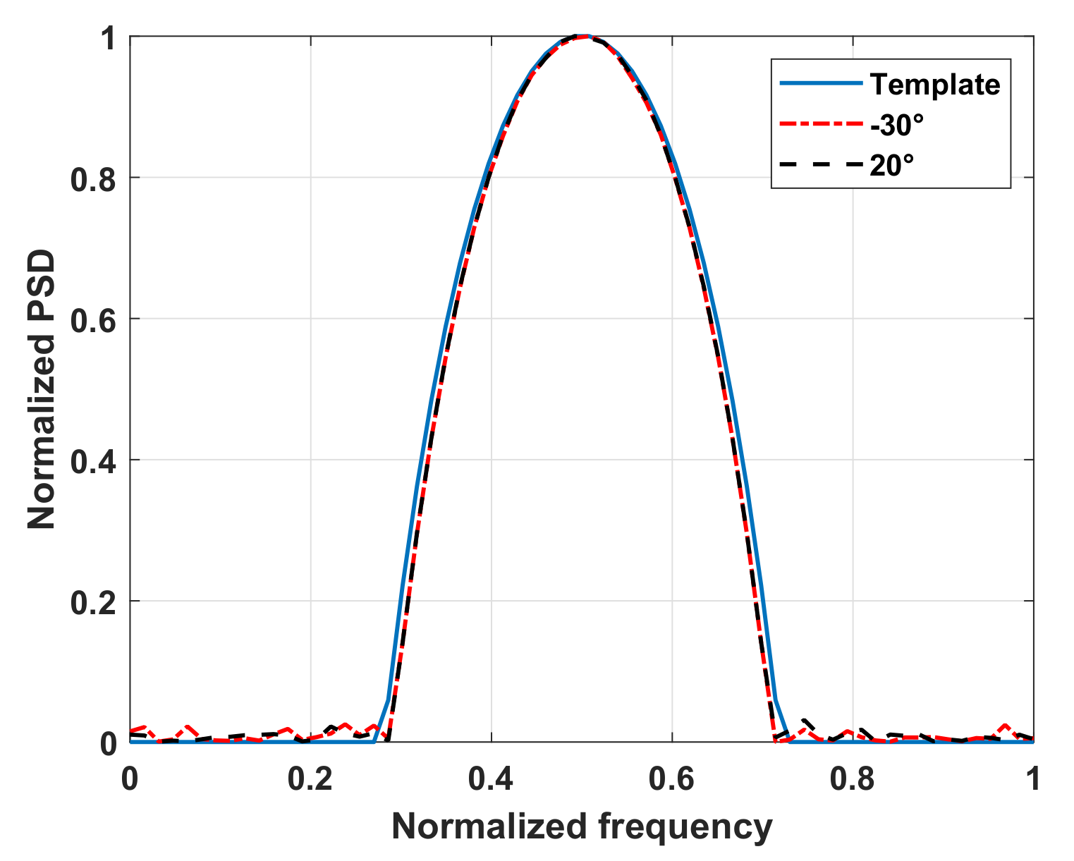
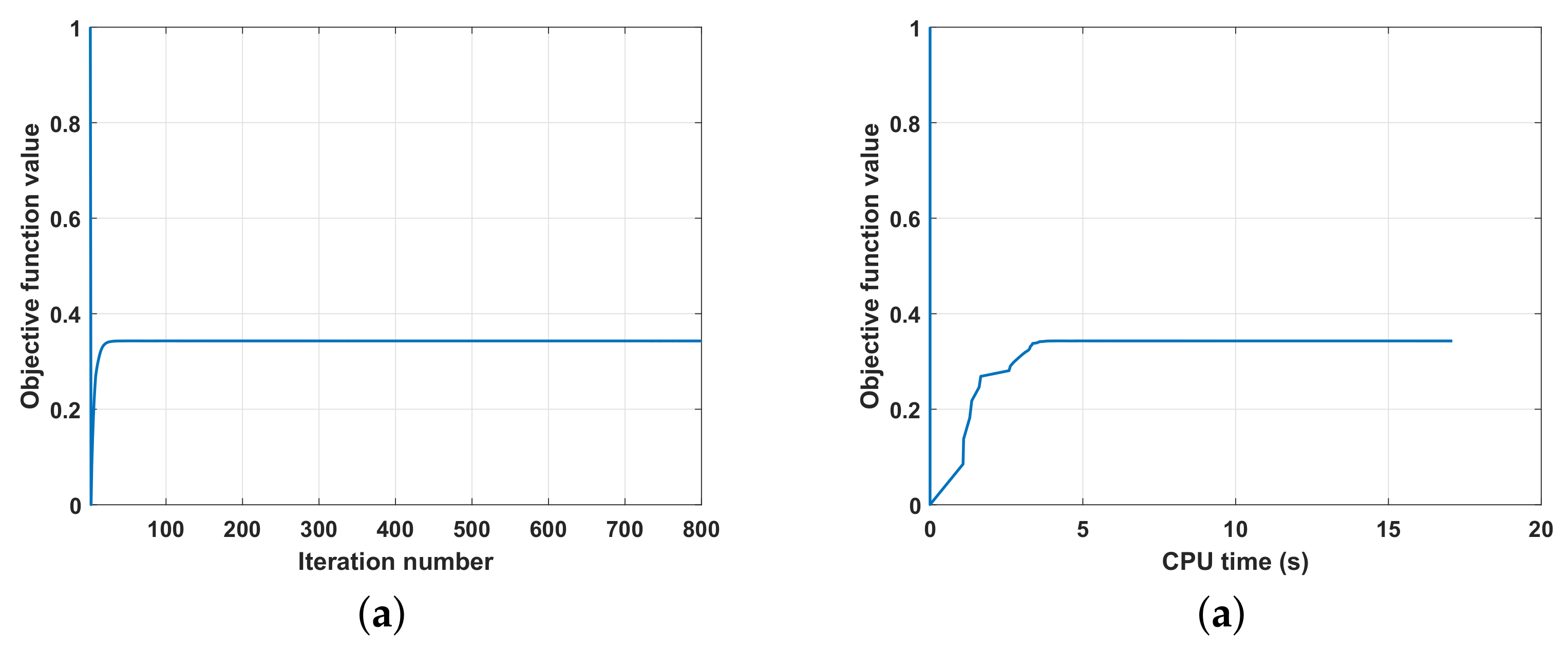
In this subsection, we conduct numerical simulations to evaluate the proposed algorithm for the PSD design of AWs. The optimal PSD template was taken from [30], which was used for ECCM. It was assumed that there were two targets located at ${\theta }_1=-{30}^{\circ }$ and ${\theta }_2={20}^{\circ }$, and according to the power allocation algorithm [17,18], radar sets ${\beta }_1={\beta }_2=0.5$. In the following simulations, we set the discrete time samples $L=64$ and set ${\alpha }_b={10}^{-2}$. In Figure 4, the transmit beampattern of the optimized waveform was shown. As seen from Figure 4, when the beams approach the key points, the sidelobe was also low. Figure 5 shows the PSD template and the PSDs of optimized AWs, where the PSDs were normalized by the maximum value. As we see, the PSDs designed by the proposed algorithm were close to the template. Figure 6a plots the performance curve of the objective function value in (38) versus the iteration number for the proposed algorithm, and Figure 6b is the corresponding performance curve of the objective function value in (38) versus the CPU time. In Figure 6, the curves are normalized by the initial objective function value. It is observed from Figure 6 that the proposed algorithm can converge as the iterations increase and the convergence speed is fast.

Figure 4. The transmit beampattern.

Figure 5. The PSDs of AWs.

Figure 6. The convergence performance of the proposed algorithm. (a) Objective function value vs. iteration number. (b) Objective function value vs. CPU time.

5.2. Joint Design of the Transmit Beampattern and AWs with Spectral Compatibility and Similarity

In this subsection, numerical simulations are conducted to evaluate the proposed algorithm for the spectral compatibility and similarity optimization of AWs. It was assumed that there were two targets located at ${\theta }_1=-{30}^{\circ }$ and ${\theta }_2={20}^{\circ }$ and radar sets ${\beta }_1=0.6$ and ${\beta }_2=0.4$. In the following simulations, we set $L=160$, ${\alpha }_b={10}^{-2}$, ${\alpha }_f={10}^{-4}$, and ${\alpha }_s=2$. The normalized occupied frequency band ${\Omega }_1=\left[0.1195,0.1824\right]$ and ${\Omega }_2=\left[0.5597,0.6226\right]$. The spectrums of the reference waveforms for AWs were obtained using an LFM spectrum in which the corresponding occupied frequency band was set to zero, and the original reference LFM had a pulse width $T_p=20\mathsf{\mu }$s and chirp rate $K_r=7.5\times {10}^6/\phantom{7.5\times {10}^6{T}_p}{T}_p$.

For comparison, the method QA-ADMM in [20] was also considered here. The work [20] considered a similar problem to us. However, there are some differences between the model in [20] and that in this paper. For the transmit beampattern, the work [20] was aimed at concentrating transmit power on the mainlobe regions and ignored the transmit gain and the power control for each beam. For the similarity constraint, the work [20] focused on each waveform out of each transmit antenna. Therefore, it may not exactly be an equal comparison. In the simulations of QA-ADMM, the mainlobe regions were set as $\left[{\theta }_1-W_N^1,{\theta }_1+W_N^1\right]\cup \left[{\theta }_2-W_N^2,{\theta }_2+W_N^2\right]$, and the reference waveforms adopted the orthogonal frequency division multiplexing (OFDM) version of the above LFM waveform. The parameter to control similarity was set to one. The parameter to control peak-to-average was set to one, i.e., the CM constraint. The weight for beampattern was one, and the weights for suppressing the space-frequency bands were ten.

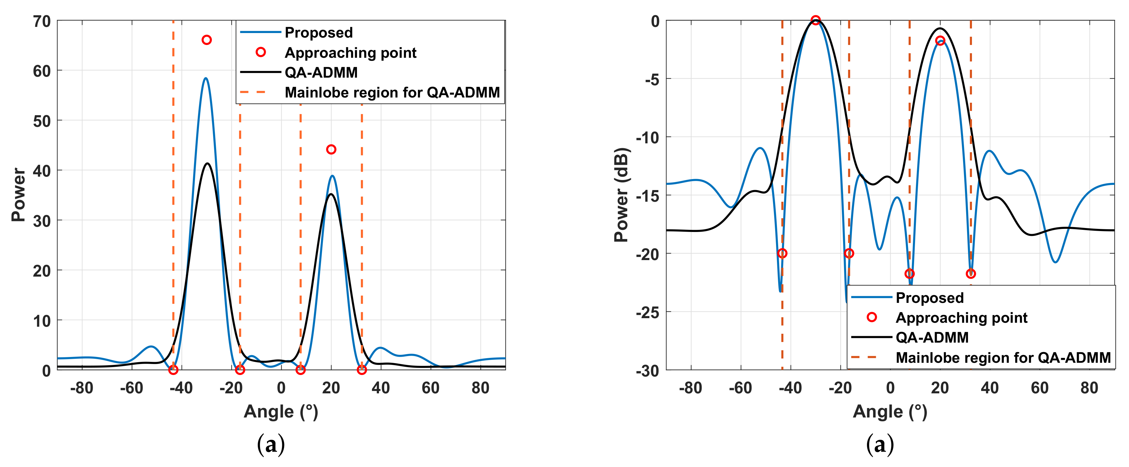
The transmit beampatterns produced by the proposed method and QA-ADMM are shown in Figure 7. The differences in the two beampatterns observed from Figure 7a are in the transmit gain and the power control for each beam. It should be noted that the QA-ADMM cannot control the power in each mainlobe region. In Figure 7b, the normalized transmit beampatterns are shown in dB, and we can see that the proposed method can accurately control the beamwidth and the power ratio of beams.

Figure 7. The transmit beampattern. (a) The original transmit beampattern. (b) The normalized transmit beampattern in dB.

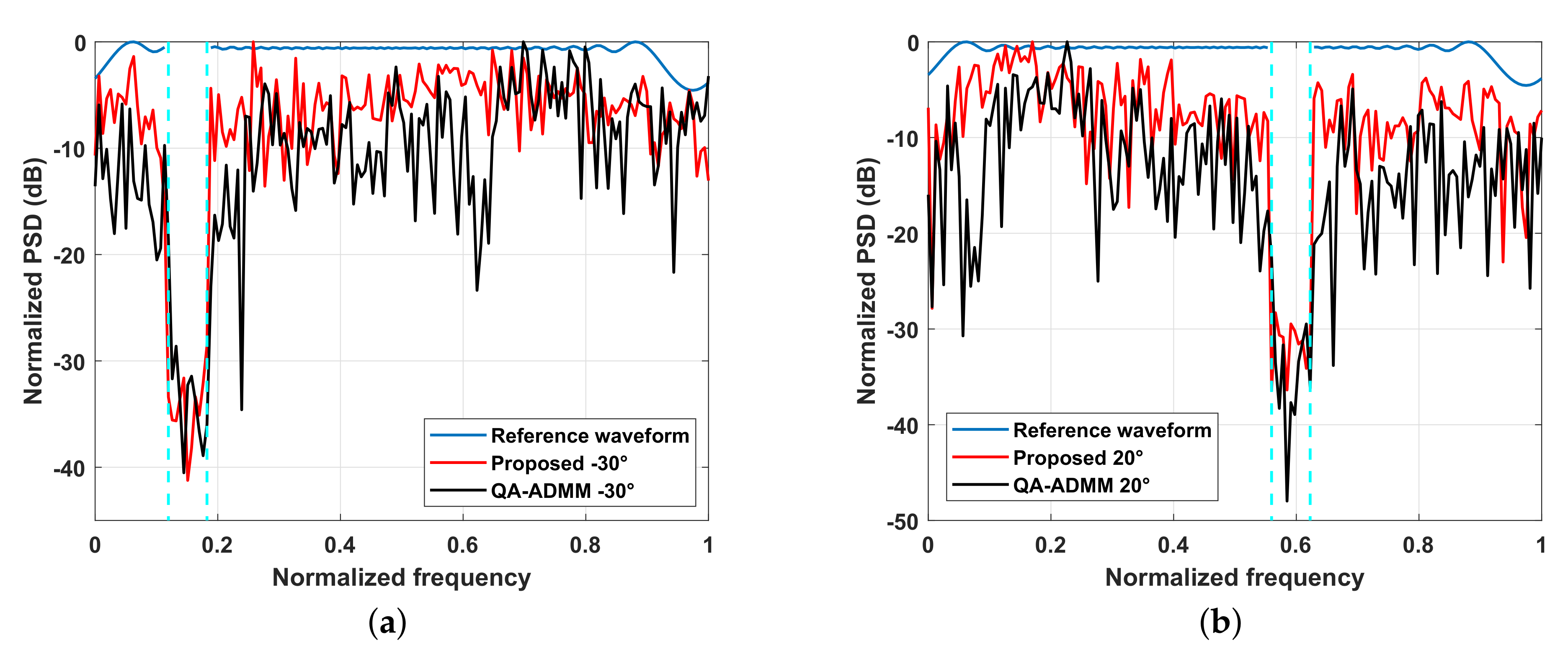
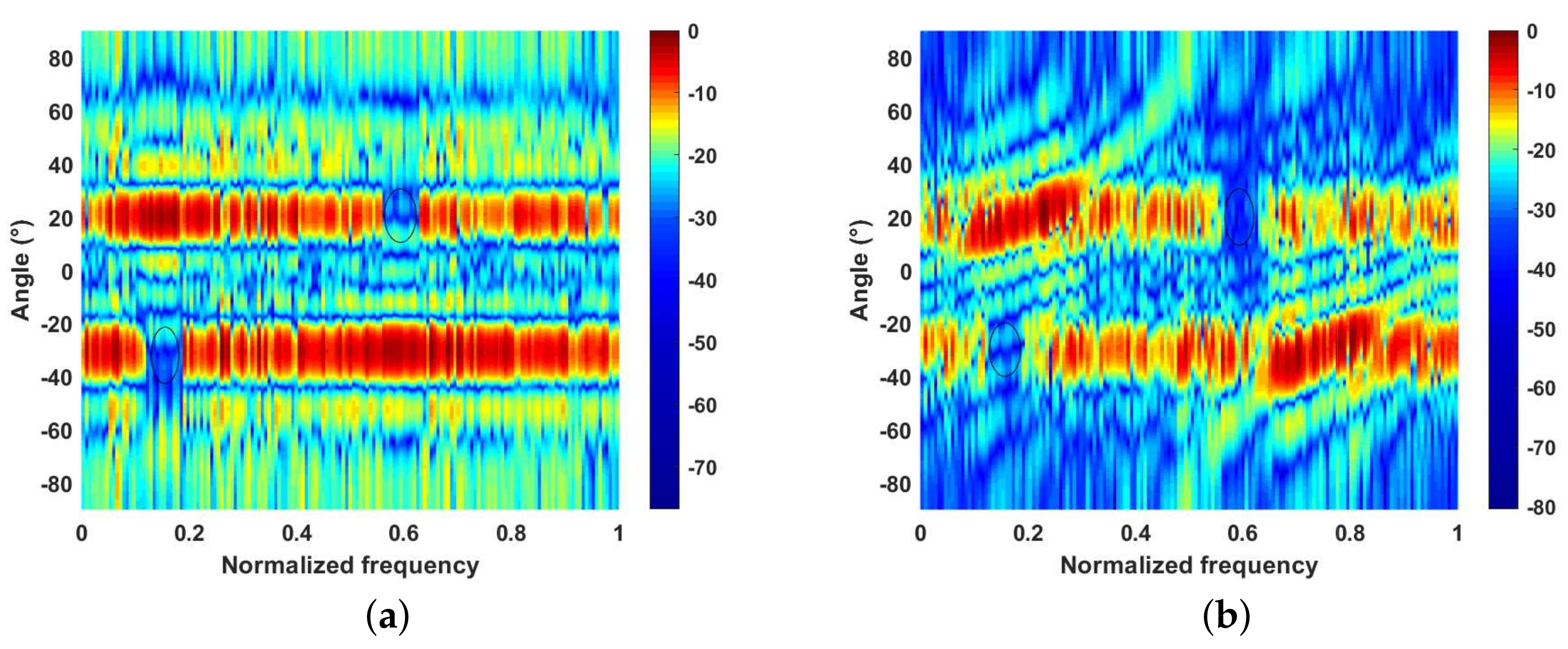
In Figure 8, we show the PSDs of the reference waveforms and the AWs produced by the proposed method and the QA-ADMM. It can be seen that notches at the occupied frequency bands can be formed using both methods. It should be noted that the QA-ADMM directly suppresses the space–frequency band. Therefore, the power distributions in the space–frequency domain of the optimized waveforms are shown in Figure 9. From Figure 9, we can see that even though only the AWs were optimized, the proposed method can obtain similar space–frequency band suppression as the QA-ADMM, and the power in the mainlobe region was more even. Moreover, we can observe from Figure 2 that the receive beamforming would narrow the mainlobe width, and the suppression of AWs on the occupied space–frequency bands would be enhanced.

Figure 8. The PSDs of reference waveforms and the AWs. (a) The PSDs of reference waveforms and the AWs at $-{30}^{\circ }$. (b) The PSDs of reference waveforms and the AWs at ${20}^{\circ }$.

Figure 9. The power distributions in the space–frequency domain. (a) The result of the proposed method. (b) The result of the QA-ADMM.

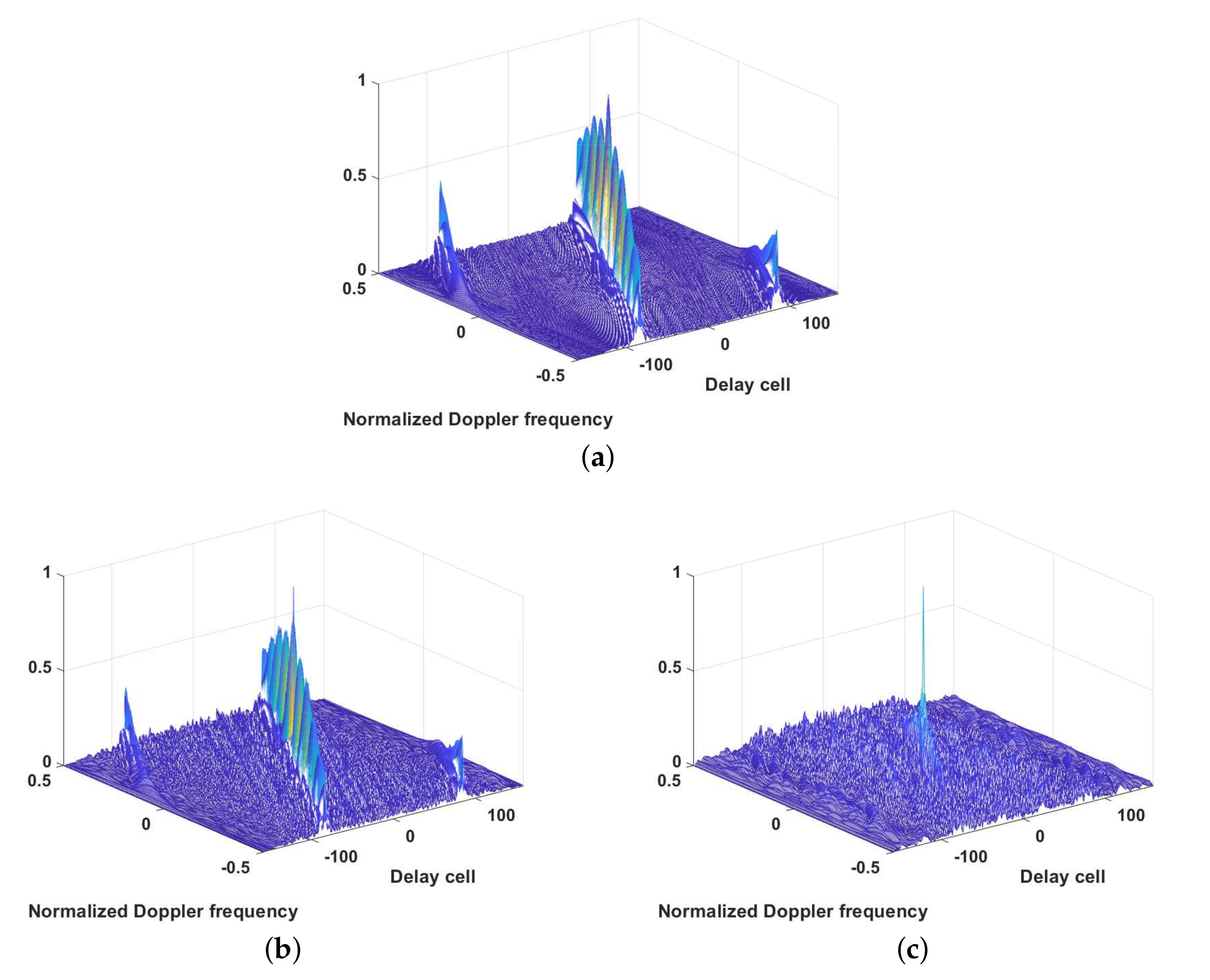
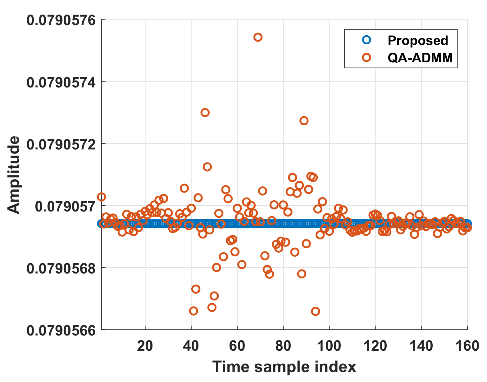
To evaluate the effect of the similarity constraint, the AFs of the AWs at $-{30}^{\circ }$ are shown in Figure 10. It can be seen that because the proposed method directly enforces the similarity constraint on the AWs, the AF of the proposed method was closer to the reference LFM. The modulus property of the designed waveform out of the first transmit antenna is given in Figure 11. Because the proposed method directly optimizes the phase, the CM property was naturally satisfied. However, for the QA-ADMM, the CM constraint may not be precisely satisfied.

Figure 10. The AFs of the optimized AWs at $-{30}^{\circ }$. (a) The reference LFM. (b) The result from the proposed method. (c) The result from the QA-ADMM.

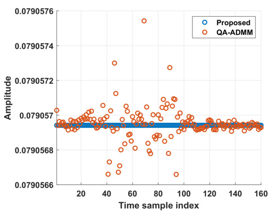
Figure 11. The modulus property of the designed waveform.

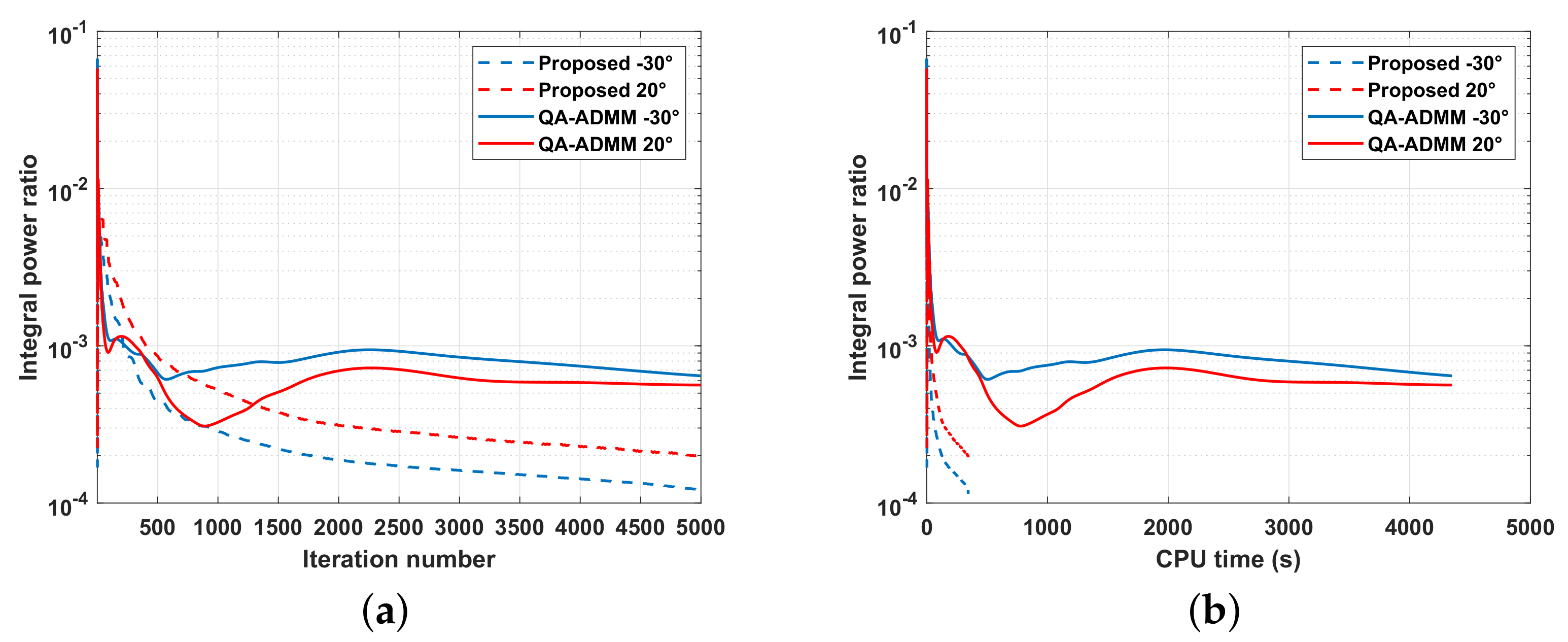
Finally, we evaluated the efficiency of each method and show the result in Figure 12. In Figure 12, the integral power ratio is defined as:

$$\begin{array}{c}\hfill \begin{array}{c}\hfill I_j=\sum _{l\in {\Omega }_j}{s}_f\left({\theta }_j,l\right)/\phantom{\sum _{l\in {\Omega }_j}{s}_f\left({\theta }_j,l\right)P\left({\theta }_j\right)}P\left({\theta }_j\right),j=1,2,\cdots ,J\end{array}\end{array}$$

(77)

and we plot the curve of the integral power ratio versus the iteration number and the corresponding curve of the integral power ratio versus the CPU time. It can be seen that the proposed method was more efficient than the QA-ADMM. It should be noted that although the integral power ratio of proposed method did not reach ${\alpha }_f$, the proposed algorithm reached the termination conditions and $\left|I_j-{\alpha }_f\right|\ll {\alpha }_f,j=1,2,\cdots J$.

Figure 12. The comparison of algorithm efficiency. (a) Integral power ratio vs. iteration number. (b) Integral power ratio vs. CPU time.

5.3. The Application of Problem (47) for AWs’ Orthogonality Design

The correlation function and the frequency spectrum of waveforms compose a Fourier transform pair. Therefore, the low cross-correlation level (CCL) between AWs can be obtained by designing the spectrum distribution between different AWs. For the auto-correlation side level (ASL), the AWs can share the low ASL property of the reference waveform due to the similarity constraint. Hence, the model (47) can also be used to design AWs with orthogonality.

According to (12), the ASL and CCL of the AW at ${\theta }_{\tilde{j}}$ are, respectively, defined as follows:

$$\begin{array}{c}\hfill \begin{array}{c}\hfill A\left(\tau ,{\theta }_{\tilde{j}}\right)={\left|\frac{{\mathbf{s}}^{\mathrm{H}}\left({\theta }_{\tilde{j}}\right){\mathbf{J}}_{\tau }\mathbf{s}\left({\theta }_{\tilde{j}}\right)}{P\left({\theta }_{\tilde{j}}\right)}\right|}^2,\begin{array}{c}\tau =-L+1,\cdots ,L-1\\ \tau \ne 0\end{array}\end{array}\end{array}$$

(78)

$$\begin{array}{c}\hfill \begin{array}{c}\hfill C\left(\tau ,{\theta }_{\tilde{j}},{\theta }_j\right)={\left|\frac{{\mathbf{s}}^{\mathrm{H}}\left({\theta }_{\tilde{j}}\right){\mathbf{J}}_{\tau }\mathbf{s}\left({\theta }_j\right)}{P\left({\theta }_{\tilde{j}}\right)}\right|}^2,\begin{array}{c}\tau =-L+1,\cdots ,L-1\\ \tilde{j}\ne j\end{array}\end{array}\end{array}$$

(79)

Further, considering the gain of receive beamforming, the CCL after receive beamforming can be given as:

$$\begin{array}{c}\hfill \begin{array}{c}\hfill C_r\left(\tau ,{\theta }_{\tilde{j}},{\theta }_j\right)=\frac{{\left|{\alpha }_{\tilde{j}j}\right|}^2}{{\left|{\alpha }_{\tilde{j}\tilde{j}}\right|}^2}{\left|\frac{{\mathbf{s}}^{\mathrm{H}}\left({\theta }_{\tilde{j}}\right){\mathbf{J}}_{\tau }\mathbf{s}\left({\theta }_j\right)}{P\left({\theta }_{\tilde{j}}\right)}\right|}^2,\begin{array}{c}\tau =-L+1,\cdots ,L-1\\ \tilde{j}\ne j\end{array}\end{array}\end{array}$$

(80)

In this subsection, it is assumed that there are two targets located at ${\theta }_1=-{30}^{\circ }$ and ${\theta }_2={20}^{\circ }$ and radar sets ${\beta }_1={\beta }_2=0.5$. We set $L=320$, ${\alpha }_b={10}^{-2}$, ${\alpha }_f={10}^{-3}$, and ${\alpha }_s=1$. The normalized occupied frequency band ${\Omega }_1=\left[0.5,1\right]$ and ${\Omega }_2=\left[0,0.5\right]$. Considering the tradeoff between Doppler tolerance and a low ASL, the nonlinear LFM (NLFM) waveform was chosen as the reference waveform. We obtained the phase of the NLFM as follows:

$$\phi \left(t\right)=\frac{\pi {\beta }_L{t}^2}{T_p}-\frac{\pi {\beta }_C{T}_p\sqrt{1-4t^2/\phantom{4t^2{T}_p^2}{T}_p^2}}{2},$$

and in the simulations below, we set $T_p=1.6\mathsf{\mu }$s, ${\beta }_L=45/\phantom{45T_p}{T}_p$, and ${\beta }_C=13/\phantom{13T_p}{T}_p$. The L-BFGS method in [24] was chosen for comparison, where the CCL and ASL were directly optimized and the transmit beampattern was designed to match a template. The beampattern template for the L-BFGS was set as:

$$\begin{array}{c}\hfill \begin{array}{c}\hfill \left\{\begin{array}{c}1,\theta \in \left[{\theta }_1-W_N^1,{\theta }_1+W_N^1\right]\cup \left[{\theta }_2-W_N^2,{\theta }_2+W_N^2\right]\hfill \\ 0,\mathrm{otherwise}\hfill \end{array}\right.\end{array}\end{array}$$

(81)

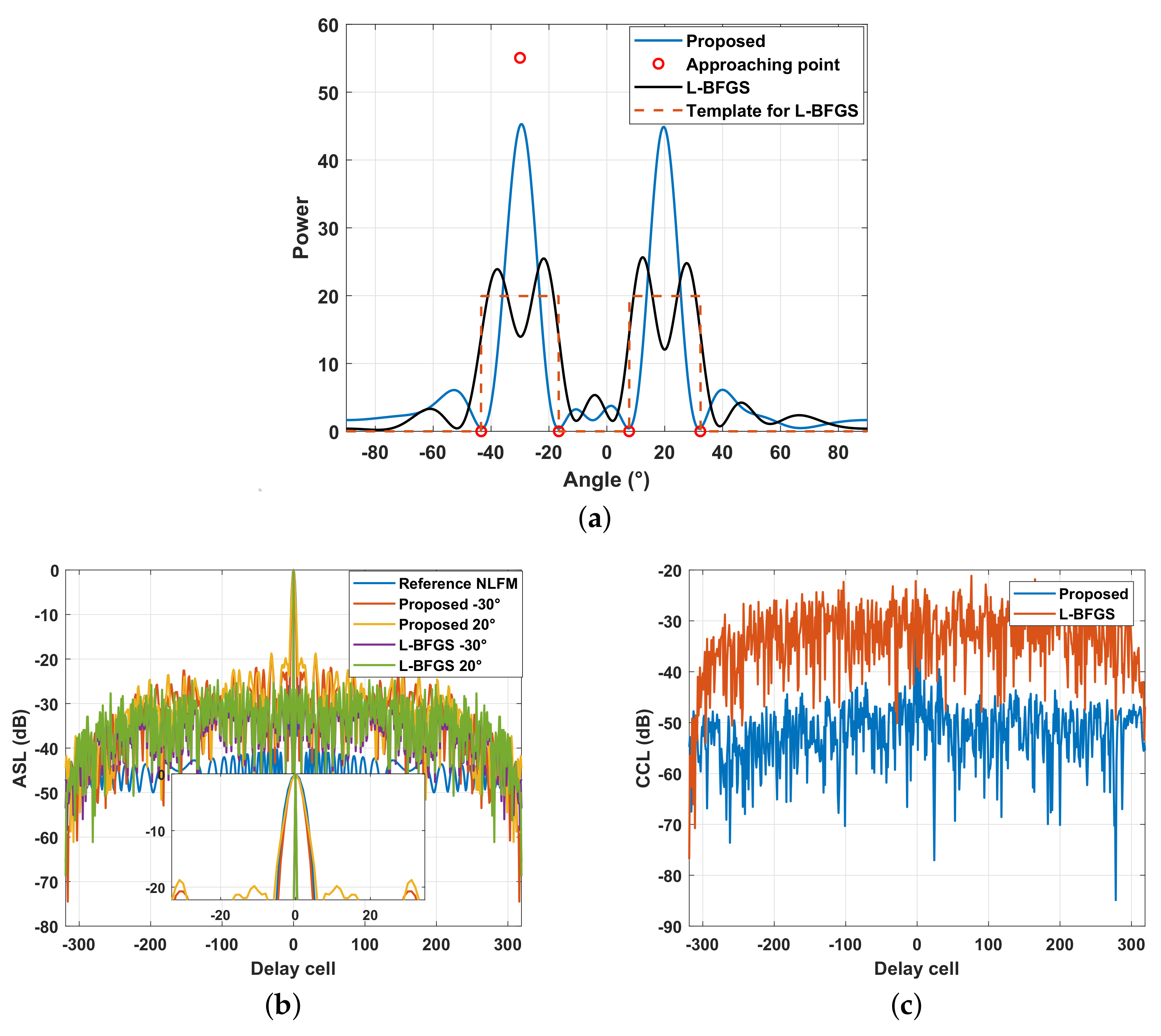
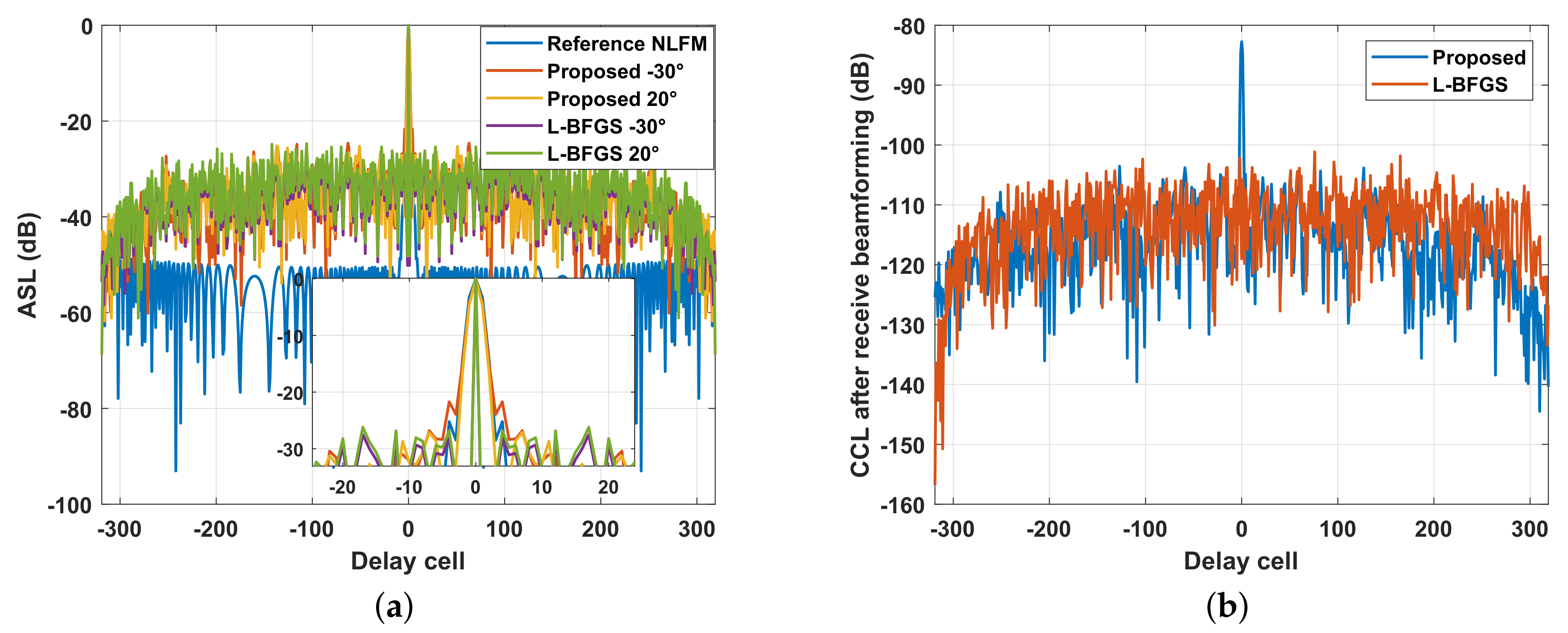
In Figure 13, we show the transmit beampattern, the ASL of AWs, and the CCL of the AW produced by the proposed method and the L-BFGS. From Figure 13a, it can be seen that the proposed method paid attention to the transmit gain and the beamwidth, while the L-BFGS focused on the template match. Figure 13b shows the ASL of AWs. It is reasonable that the ASL of the proposed method was higher than that of the L-BFGS because the L-BFGS directly optimizes the CCL and ASL. Nevertheless, the peak ASL of the proposed method was about −20 dB, and it was acceptable in most cases. In Figure 13c, because $P\left(-{30}^{\circ }\right)\approx P\left({20}^{\circ }\right)$, only the CCL of AW at $-{30}^{\circ }$ is given. It can be seen that the CCL performance of the proposed method was even better than that of the L-BFGS.

Figure 13. The results for the proposed method and the L-BFGS. (a) The transmit beampattern. (b) The ASL of AWs. (c) The CCL of AWs at $-{30}^{\circ }$.

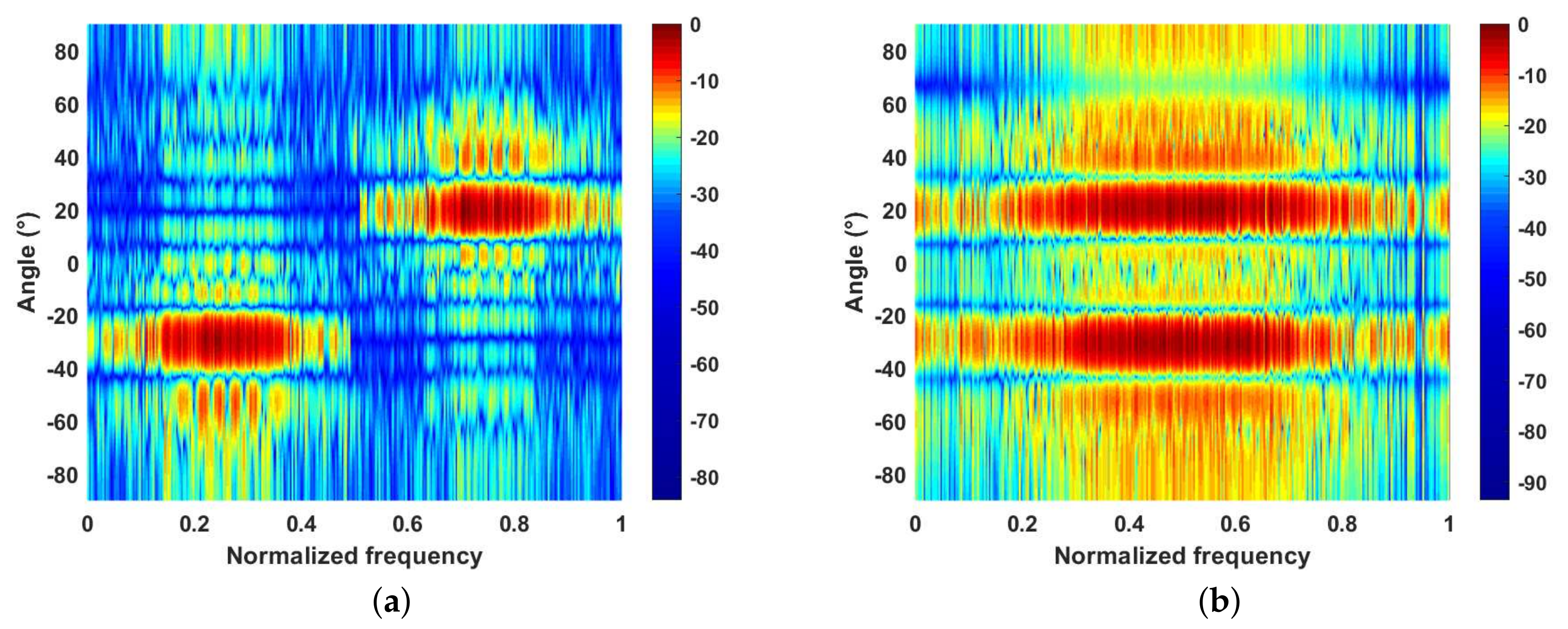
In Figure 14a, the power distribution in the space–frequency domain of optimized waveforms is shown. It can be found that the optimized AWs did not utilize the full bandwidth, which would reduce the range resolution. In fact, the CCL can be suppressed by receive beamforming [12,15], and the spectral compatibility constraint in (47) can be ignored. In the next simulation, only the ASL of AWs was optimized, i.e., only the similarity constraint was concerned, and it was assumed that the receive array with $\tilde{M}=10$ and the minimum variance distortionless response (MVDR) beamformer was adopted [15]. Besides, the reference NLFM was changed as ${\beta }_L=100/\phantom{100T_p}{T}_p$ and ${\beta }_C=25/\phantom{25T_p}{T}_p$. The power distribution in the space–frequency domain of the optimized waveforms without considering the CCL is shown in Figure 14b. It can be seen that each AW can utilize the full bandwidth. In Figure 15, we show the ASL of AWs and the CCL of AW at $-{30}^{\circ }$ after receive beamforming. It can be noticed that after ignoring the spectral compatibility constraint, the ASL of AWs produced by the proposed method was close to that of the L-BFGS, and the peak ASL was lower than −20 dB. From Figure 15b, it can be seen that the CCL after receive beamforming is tiny and can be ignored.

Figure 14. The power distributions in the space–frequency domain of waveforms optimized by the proposed method. (a) Considering the CCL. (b) Without considering the CCL.

Figure 15. The result of the proposed method and the L-BFGS after receive beamforming. (a) The ASL of AWs. (b) The CCL of AW at $-{30}^{\circ }$ after receive beamforming.

6. Discussion: Quantitative Comparisons with Existing Algorithms

In this section, the performance of the proposed algorithm is quantitatively demonstrated. All the algorithms, including the comparison algorithms, were terminated when the iteration number of 1000 was reached, and the results of each algorithm were the average of 500 trials with different random initial points. In all the tables below, ${\theta }_1=-{30}^{\circ }$, ${\theta }_2={20}^{\circ }$, and ETPI stands for the execution time per iteration.

In Table 1, we show the quantitative results corresponding to Section 5.1 to inspect the performance of the proposed algorithm for the joint design of the transmit beampattern and the PSDs of AWs. Except for the transmit antennas M and the discrete time samples L, all the other settings were the same as those in Section 5.1. To the best of our knowledge, the joint design of the transmit beampattern and the PSDs of AWs has scarcely been addressed in the literature. Therefore, only the results of the proposed algorithm are given here.

Table 1. The performance of the proposed algorithm for the joint design of the transmit beampattern and the PSDs of AWs.

M	L	$\mathit{P}\left({\mathit{\theta }}_1\right)$	$\mathit{P}\left({\mathit{\theta }}_2\right)$	OFV	ETPI (s)
10	64	48.57	48.66	0.34	0.026
20	128	193.37	193.46	0.35	0.15
30	192	437.22	437.45	0.35	0.57

In Table 1, OFV stands for the objective function value of (48), which is normalized by the objective function value of the initial point. From Table 1, we can see that, for the joint design of the transmit beampattern and the PSDs of AWs, the performance of the proposed algorithm was stable and the computational complexity was low.

In Table 2, we show the quantitative results corresponding to Section 5.2 to inspect the performance of each algorithm in jointly designing the transmit beampattern and AWs with spectral compatibility and similarity. Except for the transmit antennas M and the discrete time samples L, all other settings were the same as those in Section 5.2. The QA-ADMM algorithm was used for comparison. The integral power ratio in (77) was used to quantitatively display the suppression of AWs to the unavailable frequency band. $I_1$ and $I_2$ denote the integral power ratio of AWs at $-{30}^{\circ }$ and ${20}^{\circ }$, respectively. In order to quantitatively show the similarity of AWs, we define the following parameter:

$$\begin{array}{c}\hfill \begin{array}{c}\hfill \mathcal{S}\left(\theta \right)={∥\frac{{\mathbf{s}}_f\left(\theta \right)}{{∥{\mathbf{s}}_f\left(\theta \right)∥}_2}-\frac{\mathbf{r}\left(\theta \right)}{{∥\mathbf{r}\left(\theta \right)∥}_2}∥}_2^2\end{array}\end{array}$$

(82)

which represents the difference between the AW at $\theta$ and the reference signal, and the greater $\mathcal{S}\left(\theta \right)$ is, the worse the similarity.

Table 2. The performance of each algorithm in jointly designing the transmit beampattern and AWs with spectral compatibility and similarity.

Algorithm	M	L	$\mathit{P}\left({\mathit{\theta }}_1\right)$	$\mathit{P}\left({\mathit{\theta }}_2\right)$	${\mathit{I}}_1\times {10}^4$	${\mathit{I}}_2\times {10}^4$	$\mathcal{S}\left({\mathit{\theta }}_1\right)$	$\mathcal{S}\left({\mathit{\theta }}_2\right)$	ETPI (s)
	10	64	58.22	39.04	2.16	5.79	0.15	0.24	0.012
Proposed	20	128	233.43	153.44	2.34	4.69	0.19	0.27	0.14
	30	192	522.31	340.98	2.47	5.52	0.24	0.29	0.72
	10	64	37.28	38.06	11.8	92.6	1.52	1.78	0.11
QA-ADMM	20	128	128.31	127.73	22.3	30.7	1.64	1.98	3.13
	30	192	297.33	287.01	49.0	107	1.66	1.84	24.28

It should be noted that in Section 5.2, the power ratio of the beams was set as ${\beta }_1/\phantom{{\beta }_1{\beta }_2}{\beta }_2=1.5$. Therefore, in Table 2, we can see that $P\left({\theta }_1\right)/\phantom{P\left({\theta }_1\right)P\left({\theta }_2\right)}P\left({\theta }_2\right)\approx 1.5$ for the proposed algorithm. However, the algorithm QA-ADMM does not have this capability because it only focuses on the integral transmit power on specific regions. Moreover, the transmit gain of the QA-ADMM is lower than in the proposed algorithm.

In the proposed algorithm, the suppression to the occupied band is directly constrained by ${\alpha }_f$. However, this suppression in the QA-ADMM is concerned with a weighting coefficient, which is a qualitative optimization method. Therefore, in Table 2, $I_1$ and $I_2$ of the QA-ADMM are greater than those of the proposed algorithm. Moreover, regarding the similarity, the QA-ADMM focuses on each waveform out of each transmit antenna rather than AWs. Therefore, $\mathcal{S}\left({\theta }_1\right)$ and $\mathcal{S}\left({\theta }_2\right)$ of the QA-ADMM were also greater than that of proposed algorithm. According to the ETPI, it can be seen that the proposed algorithm is much faster than QA-ADMM.

In Table 3, we show the quantitative results corresponding to Figure 15a to inspect the performance of each algorithm in the AW orthogonality design. Except for the transmit antennas M and the discrete time samples L, all other settings were the same as those in Figure 15a. Because the CCL can be suppressed by receive beamforming, only the ASL performance was considered here. To measure the ASL performance quantitatively, we define the peak ASL (PASL) as follows:

$$\begin{array}{c}\hfill \begin{array}{c}\hfill \mathrm{PASL}=\underset{\genfrac{}{}{0pt}{}{\tau =-L+1,\cdots ,L-1}{\tau \ne 0}}{max}\left\{A\left(\tau ,{\theta }_1\right),A\left(\tau ,{\theta }_2\right)\right\}\end{array}\end{array}$$

(83)

where the definition of $A\left(\tau ,\theta \right)$ can be found in (78).

Table 3. The performance of each algorithm in the orthogonality design of AWs.

Algorithm	M	L	$\mathit{P}\left({\mathit{\theta }}_1\right)$	$\mathit{P}\left({\mathit{\theta }}_2\right)$	PASL (dB)	ETPI (s)
	10	192	46.62	47.17	−21.2	0.11
Proposed	20	256	187.49	187.94	−24.31	0.64
	30	320	410.08	414.24	−24.63	2.12
	10	192	13.82	12.02	−20.6	0.076
L-BFGS	20	256	68.15	67.38	−23.96	0.41
	30	320	70.92	69.14	−24.15	1.36

Comparing the transmit gain of the two algorithms, we can see that the L-BFGS in [24] paid too much attention to the matching of the desired template and resulted in a great loss of transmit gain. In addition, the L-BFGS realized a tradeoff between the transmit beampattern and the ASL using multiple weighting coefficients, which caused a large distortion of the transmit beampattern when the weighting coefficients were not appropriate. It can be seen that the PASL of the proposed algorithm was even lower than that of the L-BFGS. There are two reasons for this phenomenon. First, from Figure 13b and Figure 15a, we can see that the reference waveform of the proposed algorithm had a wider mainlobe than the AWs generated by the L-BFGS; that is, we obtained a lower ASL at the expense of the range resolution [7]. Second, the L-BFGS optimized the integral ASL rather than the PASL [41]. The L-BFGS had less execution time than the proposed algorithm, which is reasonable because each iteration of the proposed algorithm involved multiple iterations of the modified L-BFGS.

7. Conclusions

In this paper, the problem of the joint design of a transmit beampattern and the AW for colocated MIMO radars under the CM constraint was addressed. Two cost functions were proposed to jointly design the transmit beampattern and the AW. The first cost function considered the PSD design of the AW, and the other considered the spectral compatibility and AF of the AW. An efficient algorithm was proposed to solve the problems. Our algorithm exhibited significantly reduced computational complexity compared to the existing algorithms. Moreover, the performance of the proposed method in terms of the beampattern behavior, PSD, spectral distribution, and pulse compression property was examined through numerical simulations. A possible future direction of research might concern the extension of the proposed algorithm to deal with wideband MIMO radars.

References

- Fuhrmann, D.; San Antonio, G. Transmit beamforming for MIMO radar systems using partial signal correlation. In Proceedings of the Conference Record of the Thirty-Eighth Asilomar Conference on Signals, Systems and Computers, Pacific Grove, CA, USA, 7–10 November 2004; Volume 1, pp. 295–299. [Google Scholar] [CrossRef]
- Fishler, E.; Haimovich, A.; Blum, R.; Cimini, R.; Chizhik, D.; Valenzuela, R. Performance of MIMO radar systems: Advantages of angular diversity. In Proceedings of the Conference Record of the Thirty-Eighth Asilomar Conference on Signals, Systems and Computers, Pacific Grove, CA, USA, 7–10 November 2004; Volume 1, pp. 305–309. [Google Scholar] [CrossRef]
- Robey, F.; Coutts, S.; Weikle, D.; McHarg, J.; Cuomo, K. MIMO radar theory and experimental results. In Proceedings of the Conference Record of the Thirty-Eighth Asilomar Conference on Signals, Systems and Computers, Pacific Grove, CA, USA, 7–10 November 2004; pp. 300–304. [Google Scholar] [CrossRef]
- Haimovich, A.M.; Blum, R.S.; Cimini, L.J. MIMO Radar with Widely Separated Antennas. IEEE Signal Process. Mag. 2008, 25, 116–129. [Google Scholar] [CrossRef]
- Li, J.; Stoica, P. MIMO Radar with Colocated Antennas. IEEE Signal Process. Mag. 2007, 24, 106–114. [Google Scholar] [CrossRef]
- Zhou, S.; Liu, H.; Hongtao Su, H.Z. Doppler sensitivity of MIMO radar waveforms. IEEE Trans. Aerosp. Electron. Syst. 2016, 52, 2091–2110. [Google Scholar] [CrossRef]
- Xu, L.; Zhou, S.; Liu, H.; Zang, H.; Ma, L. Distributed multiple-input multiple-output radar waveform and mismatched filter design with expanded mainlobe. IET Radar Sonar Navig. 2018, 12, 227–238. [Google Scholar] [CrossRef]
- Deng, H.; Geng, Z.; Himed, B. MIMO radar waveform design for transmit beamforming and orthogonality. IEEE Trans. Aerosp. Electron. Syst. 2016, 52, 1421–1433. [Google Scholar] [CrossRef]
- Khan, H.; Zhang, Y.; Ji, C.; Stevens, C.; Edwards, D.; O’Brien, D. Optimizing Polyphase Sequences for Orthogonal Netted Radar. IEEE Signal Process. Lett. 2006, 13, 589–592. [Google Scholar] [CrossRef]
- Li, H.; Zhao, Y.; Cheng, Z.; Feng, D. Correlated LFM Waveform Set Design for MIMO Radar Transmit Beampattern. IEEE Geosci. Remote. Sens. Lett. 2017, 14, 329–333. [Google Scholar] [CrossRef]
- Cheng, Z.; He, Z.; Zhang, S.; Jian, L. Constant Modulus Waveform Design for MIMO Radar Transmit Beampattern. IEEE Trans. Signal Process. 2017, 65, 4912–4923. [Google Scholar] [CrossRef]
- Liu, H.; Zhou, S.; Zang, H.; Cao, Y. Two waveform design criteria for colocated MIMO radar. In Proceedings of the 2014 International Radar Conference, Lille, France, 13–17 October 2014; pp. 1–5. [Google Scholar] [CrossRef]
- Song, J.; Babu, P.; Palomar, D.P. Sequence Set Design with Good Correlation Properties Via Majorization-Minimization. IEEE Trans. Signal Process. 2016, 64, 2866–2879. [Google Scholar] [CrossRef] [Green Version]
- Stoica, P.; He, H.; Li, J. New Algorithms for Designing Unimodular Sequences with Good Correlation Properties. IEEE Trans. Signal Process. 2009, 57, 1415–1425. [Google Scholar] [CrossRef] [Green Version]
- Friedlander, B. On Transmit Beamforming for MIMO Radar. IEEE Trans. Aerosp. Electron. Syst. 2012, 48, 3376–3388. [Google Scholar] [CrossRef]
- Shi, J.; Bo, J.; Liu, H.; Ming, F.; Yan, J. Transmit design for airborne MIMO radar based on prior information. Signal Process. 2016, 128, 521–530. [Google Scholar] [CrossRef]
- Yan, J.; Liu, H.; Jiu, B.; Chen, B.; Liu, Z.; Bao, Z. Simultaneous Multibeam Resource Allocation Scheme for Multiple Target Tracking. IEEE Trans. Signal Process. 2015, 63, 3110–3122. [Google Scholar] [CrossRef]
- Yan, J.; Jiu, B.; Liu, H.; Chen, B.; Bao, Z. Prior Knowledge-Based Simultaneous Multibeam Power Allocation Algorithm for Cognitive Multiple Targets Tracking in Clutter. IEEE Trans. Signal Process. 2015, 63, 512–527. [Google Scholar] [CrossRef]
- Yu, X.; Cui, G.; Zhang, T.; Kong, L. Constrained transmit beampattern design for colocated MIMO radar. Signal Process. 2018, 144, 145–154. [Google Scholar] [CrossRef]
- Cheng, Z.; Han, C.; Liao, B.; He, Z.; Li, J. Communication-Aware Waveform Design for MIMO Radar With Good Transmit Beampattern. IEEE Trans. Signal Process. 2018, 66, 5549–5562. [Google Scholar] [CrossRef]
- Zhou, S.; Lu, J.; Varshney, P.K.; Wang, J.; Liu, H. Colocated MIMO radar waveform optimization with receive beamforming. Digit. Signal Process. 2019, 98, 102635. [Google Scholar] [CrossRef]
- Zheng, H.; Jiu, B.; Liu, H. Joint Optimization of Transmit Waveform and Receive Filter for Target Detection in MIMO Radar. IEEE Access 2019, 7, 184923–184939. [Google Scholar] [CrossRef]
- Wang, J.; Wang, Y. On the Design of Constant Modulus Probing Waveforms With Good Correlation Properties for MIMO Radar via Consensus-ADMM Approach. IEEE Trans. Signal Process. 2019, 67, 4317–4332. [Google Scholar] [CrossRef]
- Wang, Y.C.; Xu, W.; Liu, H.; Luo, Z.Q. On the Design of Constant Modulus Probing Signals for MIMO Radar. IEEE Trans. Signal Process. 2012, 60, 4432–4438. [Google Scholar] [CrossRef]
- Liu, H.; Wang, X.; Jiu, B.; Yan, J.; Wu, M.; Bao, Z. Wideband MIMO Radar Waveform Design for Multiple Target Imaging. IEEE Sens. J. 2016, 16, 8545–8556. [Google Scholar] [CrossRef]
- Gajic, A.; Radovanovic, J.; Vukovic, N.; Milanovic, V.; Boiko, D.L. Theoretical Approach to Quantum Cascade Micro-Laser Broadband Multimode Emission in Strong Magnetic Fields. Phys. Lett. A 2021, 387, 127007. [Google Scholar]
- Lionis, A.; Peppas, K.; Nistazakis, H.E.; Tsigopoulos, A.D.; Cohn, K. Experimental Performance Analysis of an Optical Communication Channel over Maritime Environment. Electronics 2020, 9, 1109. [Google Scholar] [CrossRef]
- Garlinska, M.; Pregowska, A.; Gutowska, I.; Osial, M.; Szczepanski, J. Experimental Study of the Free Space Optics Communication System Operating in the 8–12 μm Spectral Range. Electronics 2021, 10, 875. [Google Scholar] [CrossRef]
- Wang, Y.; Xu, H.; Li, D.; Wang, R.; Jin, C.; Yin, X.; Gao, S.; Mu, Q.; Xuan, L.; Cao, Z. Performance analysis of an adaptive optics system for free-space optics communication through atmospheric turbulence. Sci. Rep. 2018, 8, 1124. [Google Scholar] [CrossRef] [PubMed]
- Li, K.; Jiu, B.; Liu, H. Game Theoretic Strategies Design for Monostatic Radar and Jammer Based on Mutual Information. IEEE Access 2019, 7, 72257–72266. [Google Scholar] [CrossRef]
- Lan, X.; Li, W.; Wang, X.; Yan, J.; Jiang, M. MIMO Radar and Target Stackelberg Game in the Presence of Clutter. IEEE Sens. J. 2015, 15, 6912–6920. [Google Scholar] [CrossRef]
- Kim, H.; Goodman, N.A.; Lee, C.K.; Yang, S. Improved waveform design for radar target classification. Electron. Lett. 2017, 53, 879–881. [Google Scholar] [CrossRef] [Green Version]
- Garren, D.A.; Odom, A.C.; Osborn, M.K.; Goldstein, J.S.; Pillai, S.U.; Guerci, J.R. Full-polarization matched-illumination for target detection and identification. IEEE Trans. Aerosp. Electron. Syst. 2002, 38, 824–837. [Google Scholar] [CrossRef]
- Tang, B.; Liang, J. Efficient Algorithms for Synthesizing Probing Waveforms With Desired Spectral Shapes. IEEE Trans. Aerosp. Electron. Syst. 2019, 55, 1174–1189. [Google Scholar] [CrossRef]
- Rowe, W.; Stoica, P.; Li, J. Spectrally Constrained Waveform Design [sp Tips Tricks]. IEEE Signal Process. Mag. 2014, 31, 157–162. [Google Scholar] [CrossRef]
- Bo, T.; Jian, L.; Junli, L. Alternating direction method of multipliers for radar waveform design in spectrally crowded environments. Signal Process. 2018, 142, 398–402. [Google Scholar]
- Boyd, S.; Parikh, N.; Chu, E.; Peleato, B.; Eckstein, J. Distributed Optimization and Statistical Learning via the Alternating Direction Method of Multipliers. Found. Trends Mach. Learn. 2011, 3, 1–122. [Google Scholar] [CrossRef]
- Xiao, Y.; Li, T.F.; Wei, Z.X. Global Convergence of a Modified Limited Memory BFGS Method for Non-convex Minimization. Acta Math. Appl. Sin. 2013, 29. [Google Scholar] [CrossRef]
- Bo, J.; Liu, H.; Xu, W.; Lei, Z.; Wang, Y.; Bo, C. Knowledge-Based Spatial-Temporal Hierarchical MIMO Radar Waveform Design Method for Target Detection in Heterogeneous Clutter Zone. IEEE Trans. Signal Process. 2014, 63, 543–554. [Google Scholar]
- Boyd, S.; Vandenberghe, L. Convex Optimization; Cambridge University Press: Cambridge, UK, 2004. [Google Scholar]
- Song, J.; Babu, P.; Palomar, D.P. Sequence Design to Minimize the Weighted Integrated and Peak Sidelobe Levels. IEEE Trans. Signal Process. 2016, 64, 2051–2064. [Google Scholar] [CrossRef] [Green Version]
Publisher’s Note: MDPI stays neutral with regard to jurisdictional claims in published maps and institutional affiliations. |
© 2021 by the authors. Licensee MDPI, Basel, Switzerland. This article is an open access article distributed under the terms and conditions of the Creative Commons Attribution (CC BY) license (https://creativecommons.org/licenses/by/4.0/).