Abstract
The capacity of terrestrial ecosystems to sequester carbon dioxide (CO2) from the atmosphere is expected to be altered by climate change and CO2 fertilization, but this projection is limited by our understanding of how the soil system interacts with plants. Understanding the soil–vegetation interactions is essential to assess the magnitude and response of terrestrial ecosystems to the changing climate. Here, we used soil profile and satellite data to explore the role that soil properties play in regulating water and carbon use by plants. Data obtained for 19 terrestrial ecosystem sites in a warm temperate and humid climate were used to investigate the relationship between remotely sensed data and soil physical and chemical properties. Classification and regression tree results showed that in situ soil carbon isotope (δ13C), and soil order were significant predictors (r2 = 0.39, mean absolute error (MAE) = 0 of 0.175 gC/KgH2O) of remotely sensed water use efficiency (WUE) based on the Moderate Resolution Imaging Spectroradiometer (MODIS). Soil extractable calcium (Ca), and land cover type were significant predictors of remotely sensed carbon use efficiency (CUE) based on MODIS and Landsat data-(r2 = 0.64–0.78, MAE = 0.04–0.06). We used gross primary productivity (GPP) derived from solar-induced fluorescence (SIF) data, based on the Orbiting Carbon Observatory-2 (OCO-2), to calculate WUE and CUE (referred to as WUESIF and CUESIF, respectively) for our study sites. The regression tree analysis revealed that soil organic matter and soil extractable magnesium (Mg), δ13C, and soil silt content were the important predictors of both WUESIF (r2 = 0.19, MAE = 0.64 gC/KgH2O) and CUESIF (r2 = 0.45, MAE = 0.1), respectively. Our results revealed the importance of soil extractable Ca, soil carbon (S13C is a facet of soil carbon content), and soil organic matter predicting CUE and WUE. Insights gained from this study highlighted the importance of biotic and abiotic factors regulating plant and soil interactions. These types of data are timely and critical for accurate predictions of how terrestrial ecosystems respond to climate change.
1. Introduction
Plant growth is tightly coupled with soil nutrients, particularly nitrogen (N) and phosphorus (P) [1,2,3,4], and limitation of these nutrients is assumed to be one of the drivers of observed spatial variability in ecosystem carbon (C) fluxes [5,6,7], particularly terrestrial ecosystem productivity [8,9,10,11]. Soil P is also a limiting factor of global terrestrial ecosystem productivity [12,13], and studies have shown that P limitation on plant growth occurs more frequently than previously thought [3]. Because soil nutrients modify plant growth [14], a change in the soil-nutrient composition can alter plant responses to elevated atmospheric carbon dioxide (CO2) concentration and climate change [15,16,17,18,19,20].
Physical and chemical soil properties, such as texture, soil moisture content, and pH can influence soil nutrient concentration [21,22]. For instance, high soil pH can reduce the availability of soil N and P resulting in nutrient deficiencies [23,24]. Soil age is also a key factor determining nutrient content and the type of nutrients that limit vegetation productivity [25,26]. For example, older and more developed soils can be leached of important rock-derived nutrients such as P [27]. Conversely, soil N may be derived from external processes, such as atmospheric N disposition and biological N fixation. The concentrations of soil nutrients also vary with soil depth [28]. For instance, microbial activity can move nutrients upward into the root zone [29,30], while translocation and infiltration may increase the nutrient concentration with depth by moving nutrients downward. Thus, root systems and plant uptake along with hydrology and microbial communities have strong effects on the vertical distribution of soil nutrients [28,31].
Previous studies showed strong relationships between soil nutrient and vegetation carbon use efficiency (CUE) and water use efficiency (WUE) for different ecosystems [32,33,34]. However, the combined effects of multiple nutrients and soil characteristics on CUE and WUE have been rarely examined. CUE, defined as the ratio of net primary production (NPP) to gross primary production (GPP), measures the ecosystem proficiency to store absorbed atmospheric carbon (C) [9]. CUE plays an important role in regulating the terrestrial ecosystem’s carbon balance and determines the amount of carbon allocated to biomass [35]. An additional metric of plant resource economy quantifies the rate of carbon uptake per unit of water use. WUE measures the effect of water on the ecosystem to absorb atmospheric C [36] and varies with soil nutrients content [37]. WUE, a key physiological parameter linking carbon and water cycles, quantifies the amount of water that terrestrial ecosystems use relative to carbon gained [38,39]. CUE and WUE are important indicators of plants’ ability to adapt to changing environmental conditions, such as atmospheric CO2, precipitation, and temperature.
Satellite-based remote sensing of vegetation can be used to estimate global WUE and CUE from NASA’s Moderate Resolution Imaging Spectroradiometer (MODIS) GPP, evapotranspiration (ET), and NPP products starting from year 2000. The MODIS NPP and GPP algorithms were also modified to generate GPP and NPP at 30 m resolution from Landsat and meteorological data for the conterminous United States [40]. Estimates of global GPP are also available from the Max Planck Institute for Biogeochemistry (MPI-BGC) based on upscaling of eddy covariance-based measurements [41]. Currently, NASA ECOSTRESS onboard the space station is producing ET and WUE starting from July 2018 [42] and can also lead to instantaneous GPP estimates [43]. In addition, satellite-based solar-induced fluorescence (SIF) has been related to GPP [44,45,46]. All these satellite-derived data can be used to quantify WUE and CUE. For example, MODIS data have been applied to quantify the spatial variability and drivers of global WUE and CUE [39,47,48,49] and drought impacts on vegetation WUE [50,51]. Nevertheless, the linkage between satellite-derived CUE and WUE, and soil properties have been rarely examined.
This work builds on previous studies of plant-nutrient limitations by exploring multiple nutrient effects, variable soil profiles, and interactions between these factors. The larger effects of multiple nutrient additions (N, P, calcium, or Ca) on forest productivity than a single element was, revealed in a recent study of nutrient availability in northeastern US hardwood forests [27]. Additionally, a strong relationship between satellite-derived canopy greenness and soil N, aluminum (Al), and P was observed in tropical forests [52]. Moreover, many modeling experiments considered soil as a mixed column and thus relationships between soil nutrients and vegetation growth cannot be inferred for soil depth. Here, we examine how relationships of soil variables with CUE, WUE, and greenness indices vary with soil depth and with satellite sensors’ spatial resolutions. We present a novel approach combining CUE and WUE estimates from satellite GPP, NPP, ET, and SIF with soil properties to understand the regulatory mechanisms and effects of the nutrient cycles. Previous studies have shown that WUE varies with land use type, with forest having the highest WUE and croplands having the lowest WUE [39,53,54]. The relationship between CUE and land use type is more complex and is driven by climate controls, such as temperature and precipitation; CUE is higher in a drier and cooler climate than in a wet and warm climate [55]. In general, forest has lower CUE than grasslands, and crops have medium CUE values [55,56]. Based on previous studies, we hypothesize that the CUE and WUE depend on land use and depth-related soil properties. Moreover, this work elucidates how ecosystems are structured and function based on connections between aboveground vegetation productivity and soil properties.
2. Materials and Methods
2.1. Site Selection
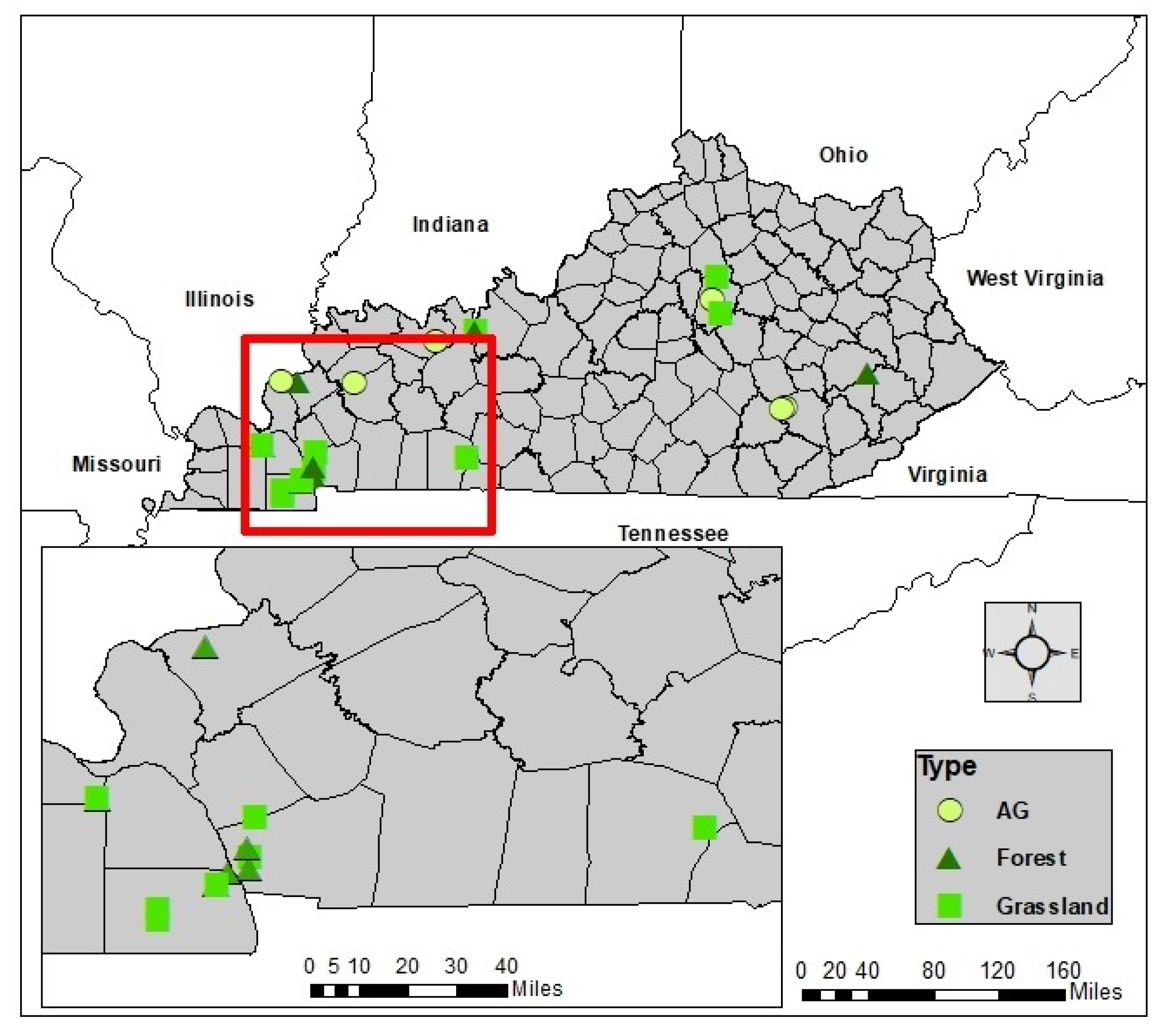
We collected soil samples from 19 sites spatially distributed across a warm temperate and fully humid climate [57] in the Commonwealth of Kentucky, USA. The region is characterized by a humid subtropical climate, with cool to moderately cold winters and warm to hot summers. The mean annual temperature ranges from 11.7 °C in the northeast to 15 °C in the southwest. The warmest month is August, while the coldest month is January. Mean annual precipitation is ~1300 mm in the south and 965 mm in the northern areas, with August the driest month and May the wettest month.
The site selection criteria consisted of two stages. Stage 1 involved the selection of potential sites that represented the major land cover types of Kentucky (i.e., agricultural, grassland, and forest). Stage 2 assessed differences in lithologic and topographic effect (slope) to assure analyses of vegetation–soil interaction were not confounded by parent material and relief. Following our site selection criteria, we identified 19 sites for soil sampling (Table 1). We limited our site selection to two soil orders: Alfisol and Ultisol, which minimized differences due to soil physical, chemical, and mineralogical properties (Figure 1). These two soil orders at the 19 sites consist of fine-grained parent material that is slight to strongly leached of nutrients in the topsoil. These soils also have clay-enriched B horizons. Unlike surrounding Inceptisols and Entisols, these two soil orders more likely reflect the surrounding long-term climate and ecological conditions. These two soil orders cover approximately 18% of the global glacial free land area according to the Soil Science Society of America (https://www.soils.org/about-soils/basics/types/, accessed on 2 June 2021).

Table 1.
Latitude, longitude, and land cover type for the 19 sites used in this study.
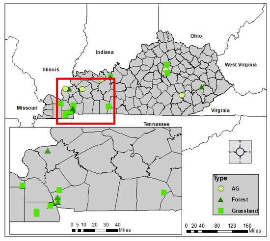
Figure 1.
Location of the 19 study sites and their land cover types in our study region, (Kentucky, USA).
2.2. Soil Physical and Chemical Analysis
Continuous soil cores were extracted using a hammer-percussion coring device and the soil horizons were described [58]. The cores were cut in half in the laboratory and an interval-sampling approach was used, where soil samples were extracted from the core every 8 ± 2 cm, to ensure that each horizon was sampled at least once. The soil physical and chemical properties were measured on samples collected to a depth of 60 cm. Particle size, oven-dry bulk density, gravimetric water content, pH, and loss on ignition (LOI) were measured for the 19 sites at Murray State University using previously established methods [59] with modifications [60]. LOI describes the variance in soil organic matter content (SOM) and is herein referred to as OM%. Soil samples were sent to the University of Kentucky Soils Characterization Lab and extractable P, C, Ca, Mg, Zn, and Fe were measured using the Mehlich-3 extraction method [61,62].
We performed soil stable isotopes analysis because they are indicators of soil C and N dynamics in an ecosystem and can be used to determine the sources of SOM and soil C turnover rates [63,64]. Soil samples were sent to the Stable Isotope Ecosystem Lab of the University of California, Merced (SIELO) for isotope analysis and elemental content of organic C and N. Splits of the soil sample (<2 mm size fraction) were prepared for stable isotope and elemental composition analysis with an initial homogenization step where samples were powdered using mortar and pestle for three to five minutes. One portion of this powdered subsample was placed in centrifuge vials and treated with 1N HCl to remove any inorganic C (calcite), which confounds the organic C signal for isotopic and elemental compositional analysis. After acidification, these subsamples were triple-rinsed in deionized water, then dried overnight at 50 °C. The other split was weighed without acid treatment to preserve δ15N values. All powdered samples were weighed to 20–40 mg (based on organic C and N content) into 5 × 9 tin capsules for stable isotope (13C/12C and 15N/14N) and organic elemental (C and N) analysis. The SIELO analyses content and isotopes of C and N with an Elemental Analyzer (Costech 4010) coupled to a Thermo Scientific Delta V Plus isotope ratio mass spectrometer via conflo IV. Reference materials for elemental and isotopic composition were run with all samples and included at least n = 3 of each Costech acetanilide, Peach Leaf (NIST 1547), and USGS 40. Reproducibility for these reference materials was <0.3‰ for both δ13C and δ15N values as well as <3% for C and N content (Table 2). Stable isotope compositions are reported with VPDB and AIR as references for δ13C and δ15N values, respectively, and in per mille (‰). All C:N ratios are reported as weight percent.
Table 2.
Summary of the soil chemical and physical properties for the study sites. Values are shown as the average for the A and B soil horizons. GR = grasslands, FR = forest, AG = agriculture.
2.3. Satellite Data
The MODIS 250 m resolution EVI (MOD13Q1) and NDVI (MOD13Q1) data and 500 m resolution ET data (MOD16A2; hereafter ET) were obtained from the USGS Earth Explorer website (https://earthexplorer.usgs.gov/, accessed on 10 April 2018) for the study sites for the year 2017. MODIS 250 m resolution GPP (8-days; hereafter GPP250) and NPP (annual; hereafter NPP250) for the year 2017 were acquired from the Terra Numerical Simulation Group (NTSG) site (http://files.ntsg.umt.edu/data/NTSG_Products/MOD17/MODIS_250/, accessed on 10 April 2018). We also acquired Landsat-derived GPP (16 days; hereafter GPP30) and NPP (annual; hereafter NPP30) data [40] at 30 m resolution from the NTSG website (http://files.ntsg.umt.edu/data/Landsat_Productivity/, accessed on 10 April 2018).
We also used the GPP product (GOSIF GPP) based on SIF derived from the Orbiting Carbon Observatory-2 (OCO-2). GOSIF is a global, OCO-2 based SIF product, while GOSIF GPP is based on GOSIF and linear relationships between GPP and SIF [65,66]. Both products are available at http://globalecology.unh.edu, accessed on 13 May 2021. GOSIF GPP data, refer to as GPPSIF hereafter were resampled from 0.05° to 250 m spatial resolution using the bilinear interpolation method to match the resolution of GPP250.
CUE based on each of the data inputs was calculated as follows:
where CUE30 is CUE estimated from Landsat 30 m GPP and NPP, CUE250 is CUE derived from MODIS 250 m GPP and NPP, and CUESIF is CUE based on MODIS 250 m NPP and GOSIF GPP. Similarly, WUE for each of the data sets was calculated as:
We used GOSIF GPP along with MODIS NPP to calculate CUE and WUE to explore how SIF-based GPP can be used to examine the relationships of WUE and CUE with soil properties.
2.4. Statistical Analysis
To identify and rank the soil chemical and physical properties that are significant in predicting CUE and WUE, we used the classification and regression trees (CART) method (the rpart package in R). The advantage of the regression tree is that it uses recursive partitioning to split the data into nodes or branches. This allows the training data to be split into groups that behave independently without the need for data stratification before analysis. For soil data analysis, whereas soil variables are the results of interdependent soil processes, the CART model is very helpful because it reveals variable interactions [67,68]. Thus, CART can help address the interdependence between soil data with depth and CUE and WUE. The predictors used to estimate WUE and CUE were land cover type, soil order, soil horizon, soil depth, layer thickness, bulk density, silt, sand, clay, OM, EC, pH-CaCl2, pH-H2O (1:1 H2O), soil organic carbon (SOC), total C, total N, C:N ratio, δ13C, δ15N, and extractable soil P, K, Ca, Mg, Zn, and Fe. Prediction errors were estimated by randomly dividing the data to 70% training (n = 80 for WUE and WUESIF; n = 72 for CUE30, n = 63 for CUE250, and n = 76 for CUESIF) and 30% testing samples (n = 35 for WUE and WUESIF; n = 31 for CUE30, n = 28 for CUE250, and n = 33 for CUESIF). The differences in the sampling sizes for the CUE data were related to the availability of satellite data for our study sites. We built the regression tree using the training sample and then pruned the tree to minimize overfitting by selecting the number of splits in the CART that is associated with a minimized cross-validated error estimate. The CART results were used to identify the soil chemical and physical variables that were important predictors for CUE and WUE. Then, the mean absolute error (MAE) was calculated by using the testing sample with the pruned CART model. We applied the CART for the 30 m and 250 m CUE and WUE to investigate the impact of spatial resolution on the results of CART. Additionally, CART was developed for CUESIF and WUESIF. Finally, we analyzed the CART results based on GPP derived from MODIS and SIF data to detect any difference in soil chemical and physical variables identified as important predictors for CUE and WUE. The reason for such comparison is that GOSIF GPP is directly estimated from SIF that is a direct measure of energy emitted by plants during photosynthesis, while MODIS GPP and NPP are based on the light use efficiency model and process-based model, respectively. Thus, they represent two different approaches to estimate CUE and WUE. To test for the effects of land cover type, soil order, soil horizon, and soil depth, we performed four additional CART analyses.: (1) excluding only land cover from the CART model (CARTnLC); (2) excluding only soil order from the CART model (CARTnSO); (3) excluding only soil horizon from the CART model (CARTnSH); and (4) excluding only soil depth from the CART model (CARTnSD). This was performed for each of the WUE and CUE data and the model with the highest r2 and lowest MAE was selected as the best model.
Soil physical and chemical properties were compared to satellite CUE and WUE. To achieve this, we summed the 8-day MODIS GPP and ET and 16-day Landsat GPP to produce annual GPP for the study sites. Both MODIS and Landsat-based NPP are directly available as annual products. Then, we used the annual data to calculate WUE and CUE at the annual timescale.
3. Results
3.1. Soil Data
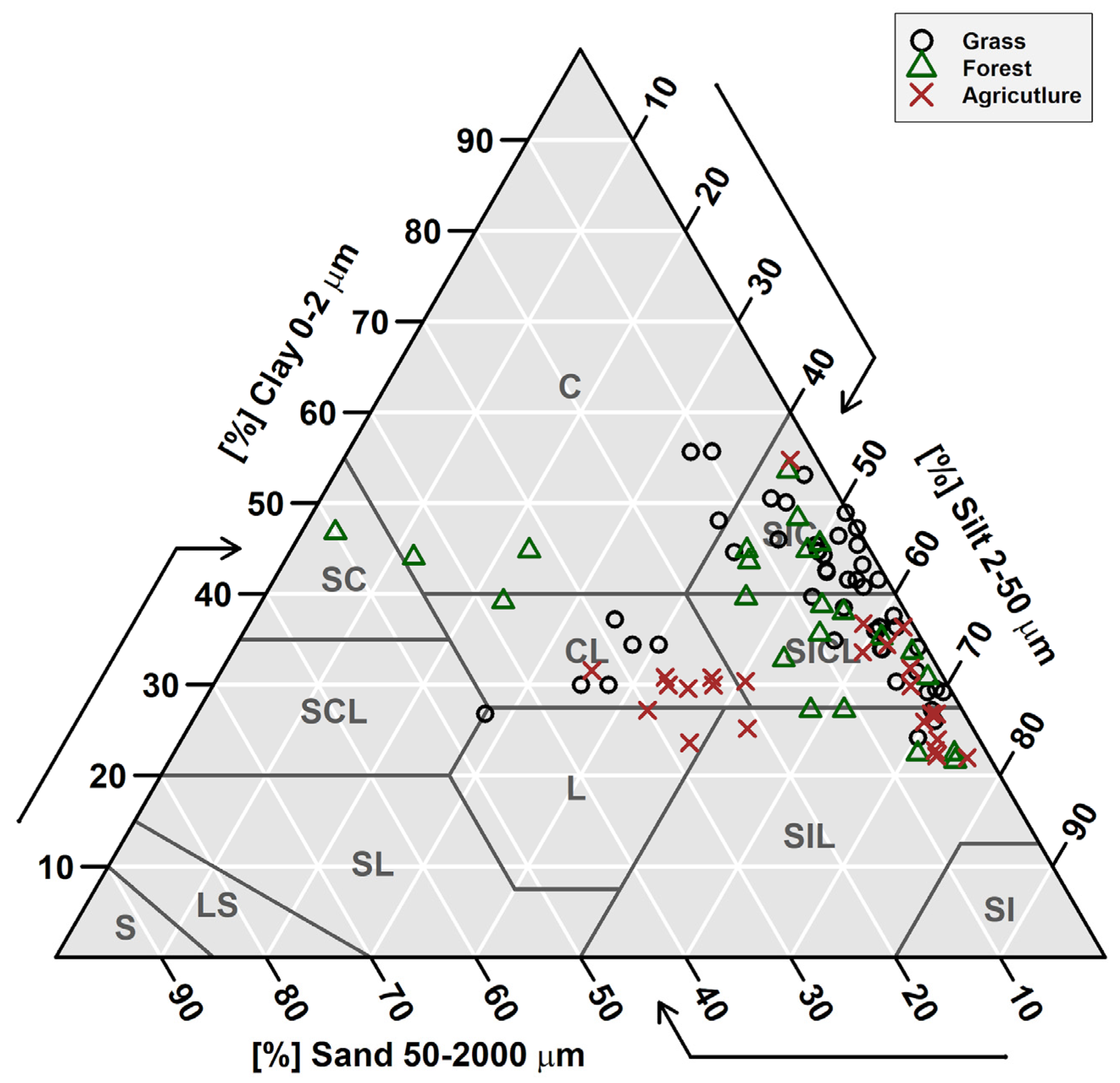
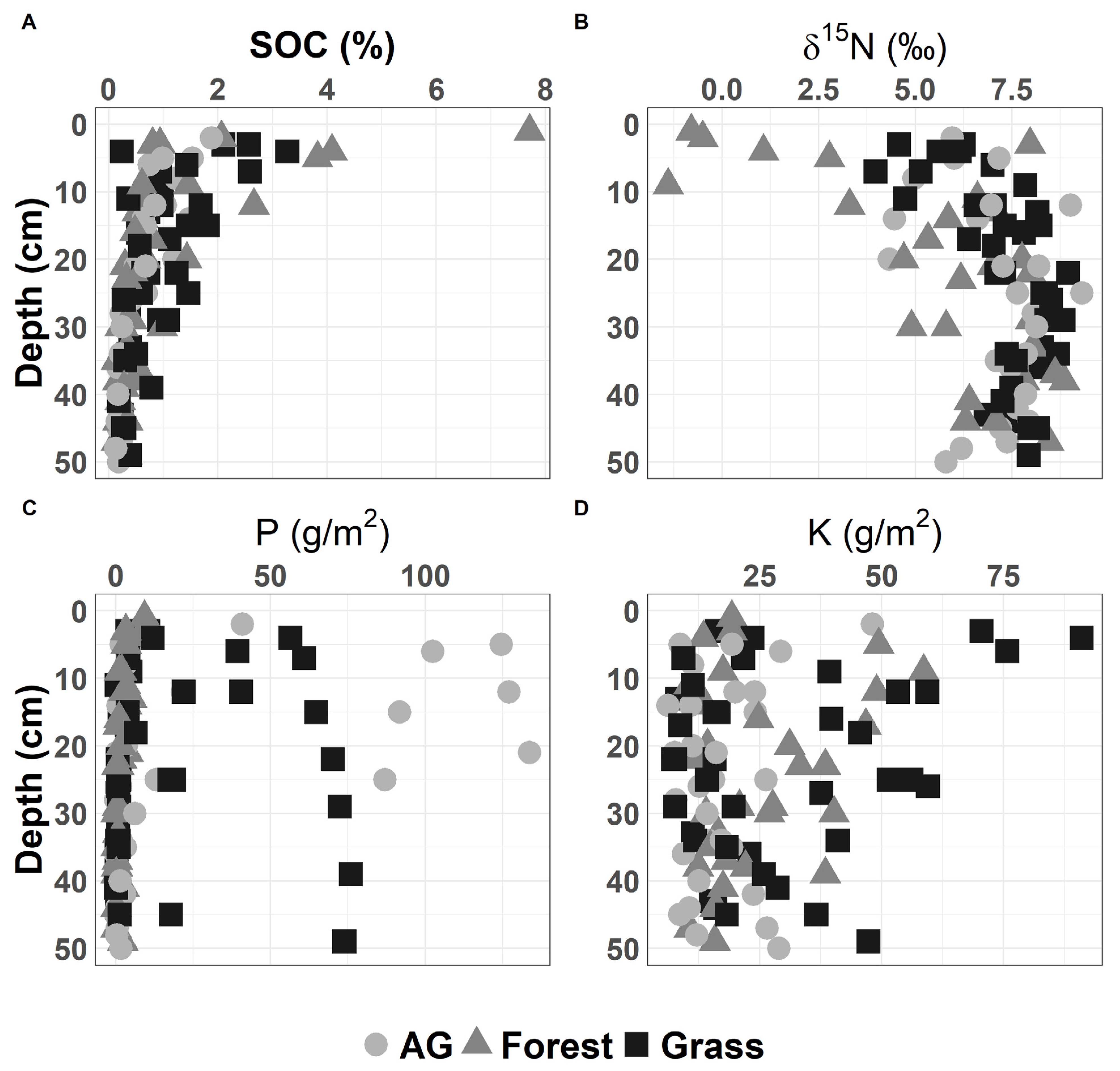
The study sites sampled for this study (7 grasslands, 6 forestlands, and 6 agricultural sites) are dominated by silty clay and silty clay loam soils (Figure 2). Forest sites showed the highest soil SOC and the lowest δ15N values in the top 10 cm of the soil, while agricultural soils had the highest P concentrations, which could be due to fertilization (Figure 3). The low forest δ15N in the top 10 cm of the soil can be related to litter inputs and low microbial processing [69] as evident in higher C:N in the soil A horizon (Table 2). In general, soil physical and chemical properties were not significantly different based on Tukey’s HSD test for land use types (i.e., forest vs. grasslands vs. agriculture) (see Supplementary Data). We note that one of our sites was formerly agricultural land (currently converted to grassland) with soil extractable P values higher than other grassland sites that were not cultivated (Figure 3C).
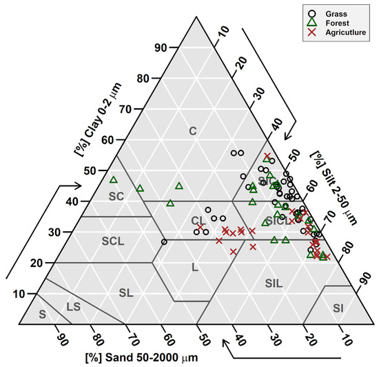
Figure 2.
Soil texture pyramid for the study sites showing the dominance of silty clay (SIC) and silty clay loam (SICL) soils. Data represents soil texture for every soil depth sampled for each site. C = clay, SC = sandy clay, SCL = sandy clay loam, SL = sandy loam, LS = loamy sand, S = sand, L = loam, CL = clay loam, SIL = silt loam, and SI = silt.

Figure 3.
Variability of soil chemical properties with soil depth for the study sites: (A) total soil carbon (%); (B) δ15N; (C) extractable phosphorus (P); (D) extractable potassium (K).
3.2. Soil Variables Versus CUE and WUE
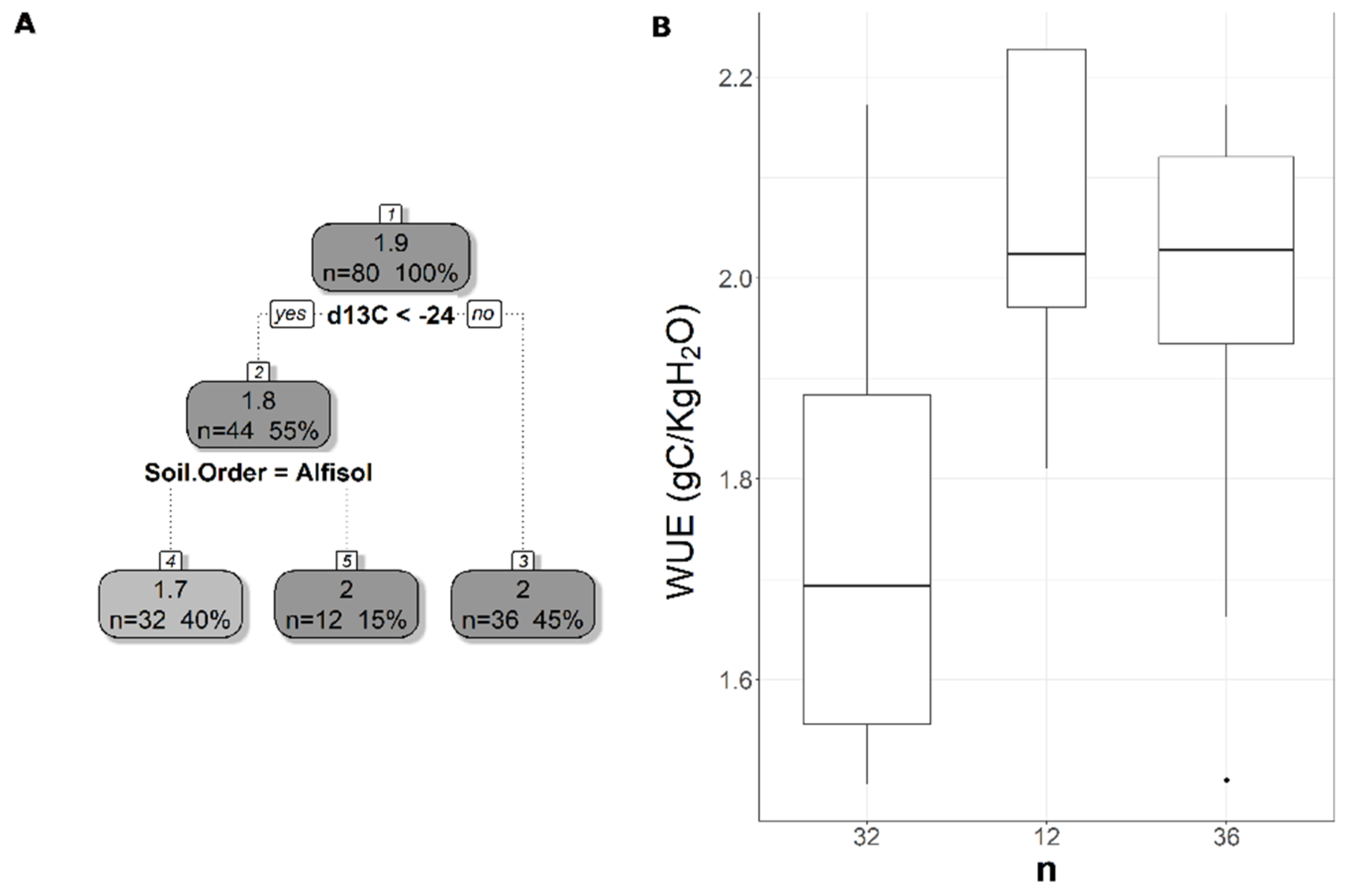
The pruned CART model for MODIS WUE showed that soil δ13C was the primary splitting node indicating the role of SOC in regulating WUE since soil δ13C is a facet of soil carbon content. MODIS WUE decreased with greater soil δ13C values (less negative) and increased with lower soil δ13C values (Figure 4A). The second split was soil order Alfisol that decreased MODIS WUE (Figure 4A), indicating lower WUE in Alfisol soils. Soil OM was the only split for WUESIF, showing a negative relationship between soil OM and WUESIF (Figure 5A). Table 3 shows the r2 and MAE values for each of the CART models developed to address the impacts of land cover, soil order, soil horizon, and soil depth. The model with the best model was the one with land cover excluded (CARTnLC) from the analysis for MODIS WUE with r2 of 0.39 and MAE of 0.17 gC/KgH2O (Table 3). The WUESIF models showed the highest MAE when all the soil variables were included (Table 3), and thus we selected the model with land cover excluded (CARTnLC) (r2 = 0.19, MAE = 0.64 gC/KgH2O) (Table 3). We found that MODIS WUE outperformed WUESIF likely because MODIS had finer spatial resolution (250 m) than the GOSIF GPP (0.05°).
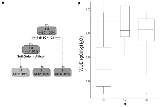
Figure 4.
Pruned regression tree for (A) MODIS-based WUE predicted as a function of two significant variables. The number in boxes 1 and 2 represent the mean CUESIF of the node, n values represent the terminal node size, soil variables names under the boxes represent the splitting criterion, and the numbers in boxes 3–5 represent the mean estimated CUE. Note that the position of “yes” and “no” at each split represents the decision split at each node. (B) Boxplots showing the distribution of WUE in each terminal node in the regression tree. The model has r2 of 0.39 and a MAE of 0.175 gC/KgH2O for WUE.
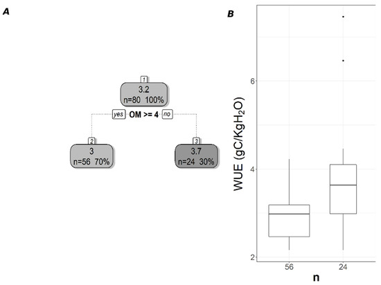
Figure 5.
Pruned regression tree for (A) WUESIF predicted as a function of one significant variable. The number in box 1 represents the mean WUESIF of the node, n value represents the terminal node size, soil variables names under the boxes represent the splitting criterion, and the numbers in boxes 2 and 3 represent the mean estimated CUE. Note that the position of “yes” and “no” at each split represents the decision split at each node. (B) Boxplots showing the distribution of WUE in each terminal branch in the regression tree. The model has r2 of 0.19 and MAE of 0.64 gC/KgH2O for WUE.
Table 3.
Summary of CART r2 and MAE (gC/KgH2O for WUE) for the CART models. The models with the highest r2 and lowest MAE are highlighted in bold. CART = all soil variables used; CARTnLC = land cover excluded from the analysis; CARTnSO = soil order excluded from the analysis; CARTnSH = soil horizon excluded from the analysis; CARTnSD = soil depth excluded from the analysis.
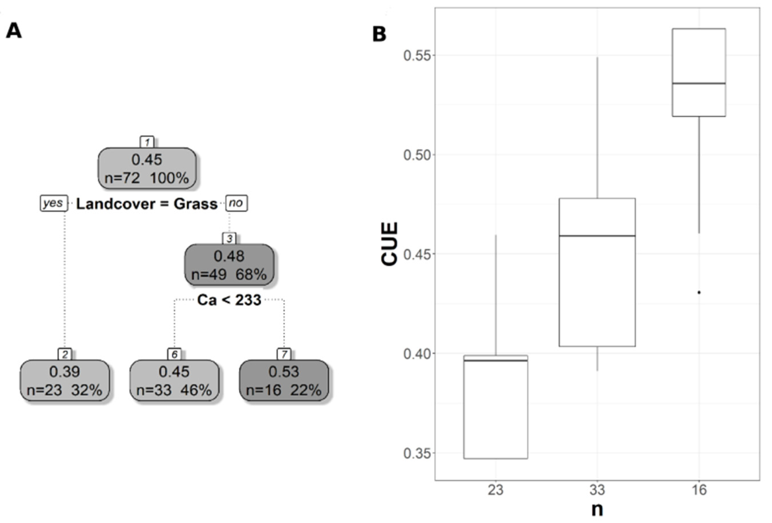
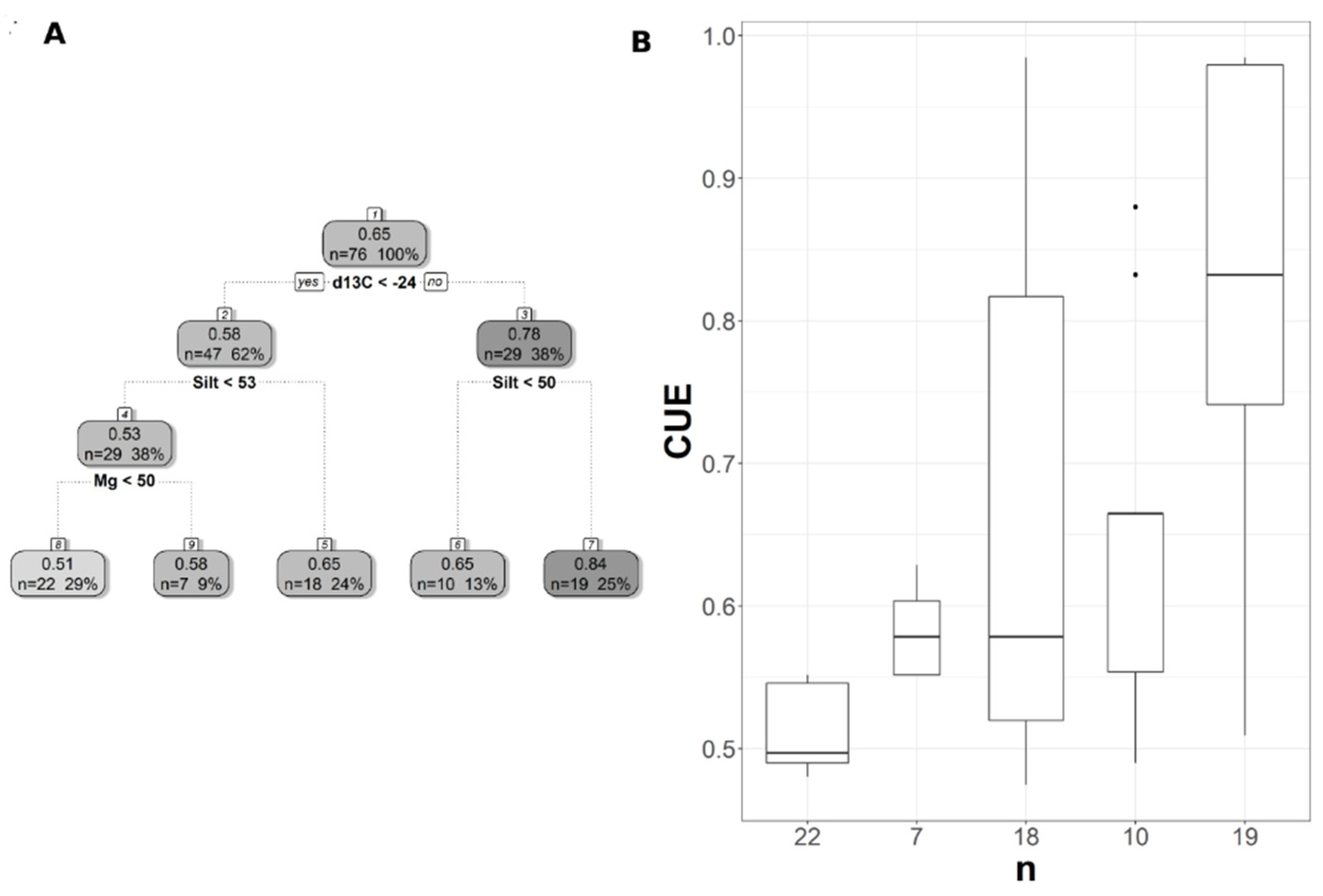
The pruned CART model for CUE30 showed that land cover was the first split, grassland being the main land cover type in the first split (Figure 6A). The second split was soil extractable Ca that showed a negative relationship with CUE30, with CUE30 increasing at lower Ca values (Figure 6A), and the CART model had r2 of 0.64 and MAE of 0.04 (Table 3). Land cover was the first split and the most important predictor for CUE250, but with the forest as the land cover predictor rather than a grassland as in CUE30 (Figure 7A). CUE250 decreased with forest with higher soil extractable Ca (Figure 7A), and the model had r2 of 0.78 and MAE of 0.06 (Table 3). Since the difference between the original CART and CARTnSH for CUE250 was almost identical, we decided to use the model that included all the soil variables (Table 3). The pruned CART model for CUESIF showed that soil δ13C was the first split showing a positive relationship with CUESIF, that the second split was soil silt content with lower CUESIF at lower soil silt content, and that the third split was soil extractable Mg that a positive relation with CUESIF (Figure 8A); the model had r2 of 0.45 and MAE of 0.1 (Table 3). The variable importance plots for the CART models are shown in the Supplementary Figures S1–S5. As expected, soil order and soil δ13C were the most important predictors of WUE (Figure S1), while OM was the most powerful predictor of WUESIF (Figure S2). Land cover was the most important predictor of CUE30 and CUE250 (Figures S3 and S4). Soil δ13C was the most important predictor of CUESIF (Figure S5). It is important to note that all other soil variables had some amount of predictive capacity for both WUE and CUE (Figures S1–S5).

Figure 6.
Pruned regression tree for (A) Landsat-based CUE predicted as a function of two significant variables. The number in boxes 1 and 3 represent the mean CUE of the node, the n value represents the terminal node size, soil variables names under the boxes represent the splitting criterion, and the numbers in boxes 2, 6, and 7 represent the mean estimated CUE. Note that the position of “yes” and “no” at each split represents the decision split at each node. (B) Boxplots showing the distribution of CUE in each terminal node in the regression tree. The model has r2 of 0.64 and MAE of 0.04 for CUE.
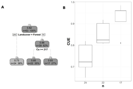
Figure 7.
Pruned regression tree for (A) MODIS CUE predicted as a function of two significant variables The number in boxes 1 and 3 represent the mean CUE of the node, n value represents the terminal node size, soil variables names under the boxes represent the splitting criterion, and the numbers in boxes 2, 6, and 7 represent the mean estimated CUE. Note that the position of “yes” and “no” at each split represents the decision split at each node. (B) Boxplots showing the distribution of CUE in each terminal branch in the regression tree. The model has r2 of 0.78 and MAE of 0.06.
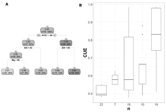
Figure 8.
Pruned regression tree for (A) CUESIF predicted as a function of three significant variables. The number in boxes 1–4 represents the mean CUESIF of the node, n value represents the terminal node size, soil variables names under the boxes represent the splitting criterion, and the numbers in boxes 5–9 represent the mean estimated CUE. Note that the position of “yes” and “no” at each split represents the decision split at each node. (B) Boxplots showing the distribution of CUE in each terminal branch in the regression tree. The model has r2 of 0.45 and MAE of 0.1.
3.3. Impacts of Different Productivity Measures and Spatial Resolution on the Relationship Satellite-Derived CUE and, WUE Withsoil Properties
We applied the CART for MODIS WUE and WUESIF to investigate the impacts of different productivity measures (based on the MODIS light use efficiency model vs. GPP based on OCO-2 SIF) on the CART results. There were no common variables detected between CART-MODIS and CART-SIF (Figure 4 and Figure 5). We compared GEOSIF GPP and MODIS GPP and found a low correlation (r2 = 0.19) between these two products (Figure S7). In general, GOSIF GPP values were much higher than MODIS GPP which was reported to underestimate site measured GPP, particularly for cropland [40,70]. Besides, we applied CART for Landsat CUE, MODIS CUE, and SIF-based CUE to investigate the impact of spatial resolution on the results of CART. The land cover type and soil extractable Ca were the common variables between MODIS CUE and Landsat CUE (Figure 7A and Figure 8A) highlighting the importance of these soil variables for predicting CUE. No common soil variables were detected among CUESIF, CUE30, and CUE250 (Figure 6, Figure 7 and Figure 8). This could be due to different algorithms used to estimate MODIS and Landsat GPP compared to the GPP derived from SIF and the different spatial resolutions of these data products (Table 4).
Table 4.
Summary of the GPP algorithm for the remote sensing data set used in this study.
4. Discussion
Overall, our approach is robust and applicable to our study sites given the significant relationships of soil chemical and physical properties with CUE and WUE. The recursive partitioning that CART is built upon can model WUE and CUE from soil physical and chemical properties by providing a simplified, but yet powerful perspective on the drivers of WUE and CUE. The CART models showed higher predictability for CUE than for WUE likely due to the uncertainties in MODIS ET or other environmental controls on WUE (e.g., vapor pressure deficit). Our results did not reject our hypothesis that CUE depends on the land cover type with grasslands and forest being the most important predictors of CUE30 and CUE250, respectively. Conversely, our results rejected the hypothesis that WUE is dependent on land cover type.
The CART WUE and CUE results revealed indirectly the correlations of soil δ13C and OM with soil depth. In general, OM was higher and soil δ13C values were lower in the topsoil layers and OM becomes lower and δ13C values increase with an increase in soil depth [71], which was also the case for our study sites (Figure S6). Although CART WUE and CART CUESIF models did not show that soil depth was an important predictor of WUE and CUESIF, they did reveal an indirect indication of the soil depth-related properties in regulating WUE and CUE as evident in Figure 4, Figure 5 and Figure 8. Therefore, our results failed to reject our hypothesis that WUE and CUE are independent of soil depth-related properties.
Our analysis revealed the importance of soil extractable Ca and Mg in regulating CUE and WUE and calls for more data collections and synthesis to better understand the potential role that these soil properties play in moderating the effects of climate change on CUE and WUE. Our methodology demonstrated the ability of remotely sensed data to capture the observed relationships of CUE, WUE, NDVI, and EVI with soil and provides a platform for future exploration of the soil–vegetation interactions using satellite vegetation data and in situ soil data.
The regression tree trained using MODIS data relied on soil δ13C and soil order to predict WUE (Figure 4). Soil δ13C values showed a positive correlation with WUE (Figure S4A) similar to the observed positive correlations between Leaf δ13C and intrinsic WUE [72,73]. This relationship can be attributed to the close relationship between SOC and δ13C values [71,74] and the role that SOC plays in controlling soil water availability. Regression tree analysis showed that soil order Alfisol was important for predicting WUE. This could be driven by our three sites with soil order Ultisol that on average had higher WUE than the other sites. In general, the three forest sites with soil order Ultisol had lower soil extractable Ca and K than the other sites. An increase in the uptake of soil extractable Ca and K can enhance WUE by decreasing ET [37]. We hypothesized that higher WUE in these three sites is due to an increase in the uptake of soil extractable Ca and K. We plan to measure leaf nutrient concentration data from our study sites to test this hypothesis in future studies. Soil OM was the only statistically significant predictor of WUESIF (Figure 5). Additionally, OM showed a negative correlation with WUE and can indicate structural water in clay minerals and/or SOC and can affect soil water holding capacity. This is because an increase in soil OM is critical for forming soil aggregate that can increase the soil-plant available water and the latter controls the ET rates [75]. These findings indicate that an increase in OM could lead to a decrease in WUE.
The regression trees trained using Landsat and MODIS data were very similar, with both relying on land cover and soil extractable Ca to predict CUE. Land cover was the most important predictor for CUE highlighting the difference between forest and grassland ecosystems, which was similar to the observed pattern in MODIS-derived CUE [33,55]. The importance of soil extractable Ca for predicting CUE highlighted the close interactions between plant N uptake, soil N pools, and soil extractable Ca [76,77], and an increase in soil extractable Ca increases GPP and eventually decreased CUE. The CUE increased with a decrease in soil extractable Mg because of the role that Ca plays in regulating physiological responses related to plant stress and growth [37,78]. For instance, the deficiency in soil Ca was related to an increase in root biomass and a decrease in respiration [78], which can lead to an increase in NPP and potentially CUE. The importance of the soil δ13C as a predictor of the CUESIF has not been reported before mainly because of limited site CUE data. As more soil δ13C data becomes available, more in-depth studies can potentially further probe into the linkages between soil δ13C values and vegetation WUE and CUE. The CART CUESIF model showed a positive relationship between CUESIF and soil extractable Mg. Soil Mg is involved in various processes that affect photosynthesis and plant growth, such as chlorophyll a and b production and root and shoot biomass [37,79,80]. A recent meta-analysis study found that an increase in soil extractable Mg leads to an increase in NPP and biomass [81], which can eventually increase CUE as predicted by our CART results.
The regression tree analysis revealed relationships of soil chemical and physical properties with WUE and CUE. The CART analysis allowed us to: unravel the interactions among various soil properties and their and combined effects on WUE and CUE; and to identify soil variables that are most important for predicting WUE or CUE. Our approach provided an understanding of the interrelationships within the datasets (e.g., soil depth) more easily than using, for example, simple or multiple regression analysis. It should be noted that the results shown in Figure 4, Figure 5, Figure 6, Figure 7, Figure 8 did not mean that these variables were the only soil variables important for predicting WUE and CUE, but rather that the CART method found these variables to be able to minimize the variability in WUE and CUE between all the tree nodes. Figures S1–S5 show the ranking of the importance of soil variables in predicting WUE and CUE. Thus, all the other soil variables (Figures S1–S5) had certain predictive power for WUE and CUE suggesting the need for more comprehensive soil–vegetation analysis to better untangle the complex soil–vegetation processes that underlie WUE and CUE.
All soil chemical and physical variables included in this study have direct or indirect effects on vegetation processes, including plant growth, WUE, GPP, and ET [37,79,80,82]. Soil extractable Zn and C:N ratio were the only soil variables that did not show any predictive power for either WUE or CUE. (Figures S1–S5). Soil δ15N values appeared once as a variable that had predictive power for WUE (Figure S1). Thus, for our study sites, these soil variables were not important in minimizing the errors in CUE or WUE between the CART tree nodes.
We collected soil samples from two soil orders to minimize the effects of soil order on soil chemical properties. We expect that our soil chemical and physical data to have little variability as they were collected from the center of Landsat 30 m pixels with a homogenous land cover type. This is less likely to be the case for the coarse-resolution MODIS (250 m) and GOSIF GPP (0.05°) data, as individual grid cells could contain multiple land cover types. With time, vegetation type and land use could alter soil properties and result in different soil chemical concentrations, leading to heterogeneous soil properties in a pixel with multiple land cover types. Moreover, soil chemical properties vary significantly as a function of topographic position. Although we controlled for land cover type (for Landsat data), we did not control for topographic variability. In addition, the scale mismatch between Landsat and MODIS can result in differences in the land cover type assigned for calculating GPP and NPP. Thus, MODIS GPP and NPP values might not represent the same land cover type as Landsat derived GPP and NPP. The scale mismatch among site, MODIS, and GOSIF GPP could influence the results since no common soil variables were detected between MODIS and GOSIF GPP CART results for CUE and WUE. Moreover, the difference in algorithms MODIS and GOSIF GPP products (Table 4) could have contributed to the differences in our results as evident in the low correlation between MODIS GPP and GOSIF GPP.
Finally, in implementing our approach, we limited the soil sampling to two soil orders to control for the effect of the variability in soil type on the results. Limiting our sampling to two soil orders could affect the broad application of our results. We anticipated that the observed relationships of CUE and WUE with soil chemical properties could apply to these two soil orders in different climatic regions, but more research is needed to verify the correlations that we observed. The robustness of our results is dependent on the accuracy of satellite data, used to estimate CUE and WUE. Newer, higher spatial resolution data on WUE from ECOSTRESS have the potential to significantly refine these results further. ECOSTRESS produces an operational WUE product at 70 × 70 m spatial resolution every 1–5 days from the International Space Station [42,83]. ECOSTRESS measures thermal infrared radiance, which is converted into a land surface temperature and emissivity (L2_LSTE) product; L2_LSTE is then converted into ET (L3_ET_PT-JPL) using the Priestley–Taylor Jet Propulsion Laboratory (PT-JPL) method [84]. ET is then combined with GPP from MOD17 to create the WUE product (L4_WUE); newer versions of ECOSTRESS replace MOD17 with a native 70 m GPP based on the Breathing Earth System Simulator [85]. ECOSTRESS can detect spatial variability in WUE never seen before (Figure S8). These differences are evident throughout the study region landscape, especially in relation to topography, hydrology, and land cover, and land use. Nevertheless, to our knowledge, our effort is one of the few that relate satellite data to soil properties for investigating the soil–vegetation interactions. CUE and WUE terms are important indicators of plants’ adaptability to changing environmental conditions, such as precipitation and temperature. Understanding changes in CUE and WUE is thus critical to quantify the response of the terrestrial ecosystem to climate change.
5. Conclusions
CUE and WUE are key physiological parameters linking carbon and water cycles. Understanding changes in these efficiencies is critical to quantify future terrestrial ecosystem responses to climate change. Here, we presented a different approach to understand the stand-level soil–vegetation interactions by using remotely sensed data. Data from the 19 sites representative of the major land cover types occurring in a warm-temperate and humid climate were used to investigate the capability of satellite data to derive meaningful information about the soil–vegetation interactions. The results revealed significant relationships between satellite-derived CUE and WUE and measured soil chemical properties. The CART model identified soil variables that were important to predict CUE and WUE, implying that satellite data have the potential for elucidating soil–vegetation interactions.
We have learned from this study that satellite spatial resolution was not important for more accurate detection of relationships between satellite vegetation products and soil chemical properties. Interestingly, coarser-resolution MODIS data produce the best estimates for CUE than high-resolution remote sensing products (e.g., Landsat CUE). Our study is limited by the number of sites used and the reported relationships may differ with more data or additional biomes or soil types. Nevertheless, our study represents a new approach that can be used to better understand the observed spatial variability in satellite-derived CUE and WUE data and can be used to inform land surface models about missing processes that are essential for more accurate predictions of vegetation CUE and WUE [86].
Supplementary Materials
The following are available online at https://www.mdpi.com/article/10.3390/rs13132593/s1. Figures S1–S5: Variable importance ranking based on the total reduction in mean square error (MSE) for calibrated CART CUE and WUE models, Figure S6: variability of soil carbon isotope and organic matter with soil depth, Figure S7: regression analysis for the relationship between MODIS GPP and GOSIF GPP for our study sites. Figure S8: Spatial image of WUE from ECOSTRESS. and supplementary data showing the Tukey’s HSD test for our study sites.
Author Contributions
B.E.M. and G.E.S. conceived and designed the research; B.E.M., G.E.S. and S.L.K. performed the research and analyzed and interpreted the data; B.F. collected the data and performed lab analysis; B.E.M. was responsible for the research analysis; J.B.F. produced the ECOSTRESS data; J.X. contributed the GOSIF GPP data; B.E.M., G.E.S. and S.L.K. contributed to the writing of the manuscript; H.C., J.B.F. and J.X. reviewed and revised the manuscript. All authors have read and agreed to the published version of the manuscript.
Funding
The material is based upon work supported by NASA Kentucky under NASA award No: NNX15AK28A. J.X. was supported by NASA’s Climate Indicators and Data Products for Future National Climate Assessments (award No: NNX16AG61G).
Data Availability Statement
The data presented in this study is available upon request from the corresponding author.
Acknowledgments
We thank Lance Stewart, Mallory Gerzan, Molly Karnes, Austin Johnessee, and Joalda Morancy for the field, lab, and data assistance. J.B.F. contributed to this research at the Jet Propulsion Laboratory, California Institute of Technology, under a contract with the National Aeronautics and Space Administration. Government sponsorship acknowledged. J.B.F. was supported in part by NASA programs: IDS and ECOSTRESS. Copyright 2021. All rights reserved.
Conflicts of Interest
The authors declare no conflict of interest.
References
- Chapin, F.S.; Bloom, A.J.; Field, C.B.; Waring, R.H. Plant Responses to Multiple Environmental FactorsPhysiological Ecology Provides Tools for Studying How Interacting Environmental Resources Control Plant Growth. BioScience 1987, 37, 49–57. [Google Scholar] [CrossRef]
- Fisher, J.B.; Badgley, G.; Blyth, E. Global Nutrient Limitation in Terrestrial Vegetation. Glob. Biogeochem. Cycles 2012, 26. [Google Scholar] [CrossRef]
- Niinemets, Ü.; Kull, K. Co-Limitation of Plant Primary Productivity by Nitrogen and Phosphorus in a Species-Rich Wooded Meadow on Calcareous Soils. Acta Oecologica 2005, 28, 345–356. [Google Scholar] [CrossRef]
- Schulze, E.-D.; Kelliher, F.M.; Korner, C.; Lloyd, J.; Leuning, R. Relationships Among Maximum Stomatal Conductance, Ecosystem Surface Conductance, Carbon Assimilation Rate, and Plant Nitrogen Nutrition: A Global Ecology Scaling Exercise. Annu. Rev. Ecol. Syst. 1994, 25, 629–660. [Google Scholar] [CrossRef]
- Fernández-Martínez, M.; Vicca, S.; Janssens, I.A.; Sardans, J.; Luyssaert, S.; Campioli, M.; Iii, F.S.C.; Ciais, P.; Malhi, Y.; Obersteiner, M.; et al. Nutrient Availability as the Key Regulator of Global Forest Carbon Balance. Nat. Clim. Chang. 2014, 4, 471–476. [Google Scholar] [CrossRef] [Green Version]
- Wang, Y.P.; Law, R.M.; Pak, B. A Global Model of Carbon, Nitrogen and Phosphorus Cycles for the Terrestrial Biosphere. Biogeosciences 2010, 7, 2261–2282. [Google Scholar] [CrossRef] [Green Version]
- Terrer, C.; Phillips, R.P.; Hungate, B.A.; Rosende, J.; Pett-Ridge, J.; Craig, M.E.; van Groenigen, K.J.; Keenan, T.F.; Sulman, B.N.; Stocker, B.D.; et al. A Trade-off between Plant and Soil Carbon Storage under Elevated CO2. Nature 2021, 591, 599–603. [Google Scholar] [CrossRef]
- De Vries, W.; Solberg, S.; Dobbertin, M.; Sterba, H.; Laubhann, D.; van Oijen, M.; Evans, C.; Gundersen, P.; Kros, J.; Wamelink, G.W.W.; et al. The Impact of Nitrogen Deposition on Carbon Sequestration by European Forests and Heathlands. For. Ecol. Manag. 2009, 258, 1814–1823. [Google Scholar] [CrossRef]
- Fernández-Martínez, M.; Vicca, S.; Janssens, I.A.; Luyssaert, S.; Campioli, M.; Sardans, J.; Estiarte, M.; Peñuelas, J. Spatial Variability and Controls over Biomass Stocks, Carbon Fluxes, and Resource-Use Efficiencies across Forest Ecosystems. Trees 2014, 28, 597–611. [Google Scholar] [CrossRef]
- Hungate, B.A.; Dukes, J.S.; Shaw, M.R.; Luo, Y.; Field, C.B. Nitrogen and Climate Change. Science 2003, 302, 1512–1513. [Google Scholar] [CrossRef] [PubMed] [Green Version]
- Terrer, C.; Jackson, R.B.; Prentice, I.C.; Keenan, T.F.; Kaiser, C.; Vicca, S.; Fisher, J.B.; Reich, P.B.; Stocker, B.D.; Hungate, B.A.; et al. Nitrogen and Phosphorus Constrain the CO2 Fertilization of Global Plant Biomass. Nat. Clim. Chang. 2019, 9, 684–689. [Google Scholar] [CrossRef] [Green Version]
- Vitousek, P.M.; Porder, S.; Houlton, B.Z.; Chadwick, O.A. Terrestrial Phosphorus Limitation: Mechanisms, Implications, and Nitrogen–Phosphorus Interactions. Ecol. Appl. 2010, 20, 5–15. [Google Scholar] [CrossRef] [Green Version]
- Ågren, G.I.; Wetterstedt, J.Å.M.; Billberger, M.F.K. Nutrient Limitation on Terrestrial Plant Growth—Modeling the Interaction between Nitrogen and Phosphorus. New Phytol. 2012, 194, 953–960. [Google Scholar] [CrossRef]
- Vicca, S.; Luyssaert, S.; Peñuelas, J.; Campioli, M.; Chapin, F.S.; Ciais, P.; Heinemeyer, A.; Högberg, P.; Kutsch, W.L.; Law, B.E.; et al. Fertile Forests Produce Biomass More Efficiently. Ecol. Lett. 2012, 15, 520–526. [Google Scholar] [CrossRef]
- Lanning, M.; Wang, L.; Scanlon, T.M.; Vadeboncoeur, M.A.; Adams, M.B.; Epstein, H.E.; Druckenbrod, D. Intensified Vegetation Water Use under Acid Deposition. Sci. Adv. 2019, 5, eaav5168. [Google Scholar] [CrossRef] [Green Version]
- Lu, X.; Vitousek, P.M.; Mao, Q.; Gilliam, F.S.; Luo, Y.; Zhou, G.; Zou, X.; Bai, E.; Scanlon, T.M.; Hou, E.; et al. Plant Acclimation to Long-Term High Nitrogen Deposition in an N-Rich Tropical Forest. Proc. Natl. Acad. Sci. USA 2018, 115, 5187–5192. [Google Scholar] [CrossRef] [PubMed] [Green Version]
- Ripullone, F.; Lauteri, M.; Grassi, G.; Amato, M.; Borghetti, M. Variation in Nitrogen Supply Changes Water-Use Efficiency of Pseudotsuga Menziesii and Populus × Euroamericana; a Comparison of Three Approaches to Determine Water-Use Efficiency. Tree Physiol. 2004, 24, 671–679. [Google Scholar] [CrossRef]
- Fisher, J.B.; Sitch, S.; Malhi, Y.; Fisher, R.A.; Huntingford, C.; Tan, S.-Y. Carbon Cost of Plant Nitrogen Acquisition: A Mechanistic, Globally Applicable Model of Plant Nitrogen Uptake, Retranslocation, and Fixation. Glob. Biogeochem. Cycles 2010, 24. [Google Scholar] [CrossRef] [Green Version]
- Allen, K.; Fisher, J.B.; Phillips, R.P.; Powers, J.S.; Brzostek, E.R. Modeling the Carbon Cost of Plant Nitrogen and Phosphorus Uptake Across Temperate and Tropical Forests. Front. For. Glob. Chang. 2020, 3, 43. [Google Scholar] [CrossRef]
- Brzostek, E.R.; Fisher, J.B.; Phillips, R.P. Modeling the Carbon Cost of Plant Nitrogen Acquisition: Mycorrhizal Trade-Offs and Multipath Resistance Uptake Improve Predictions of Retranslocation. J. Geophys. Res. Biogeosciences 2014, 119, 1684–1697. [Google Scholar] [CrossRef]
- Burke, I.C.; Yonker, C.M.; Parton, W.J.; Cole, C.V.; Flach, K.; Schimel, D.S. Texture, Climate, and Cultivation Effects on Soil Organic Matter Content in U.S. Grassland Soils. Soil Sci. Soc. Am. J. 1989, 53, 800–805. [Google Scholar] [CrossRef]
- Schmidt, M.W.I.; Torn, M.S.; Abiven, S.; Dittmar, T.; Guggenberger, G.; Janssens, I.A.; Kleber, M.; Kögel-Knabner, I.; Lehmann, J.; Manning, D.A.C.; et al. Persistence of Soil Organic Matter as an Ecosystem Property. Nature 2011, 478, 49–56. [Google Scholar] [CrossRef] [Green Version]
- Neina, D. The Role of Soil PH in Plant Nutrition and Soil Remediation. Appl. Environ. Soil Sci. 2019, 2019, e5794869. [Google Scholar] [CrossRef]
- Aciego Pietri, J.C.; Brookes, P.C. Nitrogen Mineralisation along a PH Gradient of a Silty Loam UK Soil. Soil Biol. Biochem. 2008, 40, 797–802. [Google Scholar] [CrossRef]
- Vitousek, P.M.; Farrington, H. Nutrient Limitation and Soil Development: Experimental Test of a Biogeochemical Theory. Biogeochemistry 1997, 37, 63–75. [Google Scholar] [CrossRef]
- Buendía, C.; Arens, S.; Hickler, T.; Higgins, S.I.; Porada, P.; Kleidon, A. On the Potential Vegetation Feedbacks That Enhance Phosphorus Availability—Insights from a Process-Based Model Linking Geological and Ecological Timescales. Biogeosciences 2014, 11, 3661–3683. [Google Scholar] [CrossRef] [Green Version]
- Vadeboncoeur, M.A. Meta-Analysis of Fertilization Experiments Indicates Multiple Limiting Nutrients in Northeastern Deciduous Forests. Can. J. For. Res. 2010, 40, 1766–1780. [Google Scholar] [CrossRef] [Green Version]
- Jobbágy, E.G.; Jackson, R.B. The Distribution of Soil Nutrients with Depth: Global Patterns and the Imprint of Plants. Biogeochemistry 2001, 53, 51–77. [Google Scholar] [CrossRef]
- Stark, J.M. Causes of Soil Nutrient Heterogeneity at Different Scales. In Exploitation of Environmental Heterogeneity by Plants; Caldwell, M.M., Pearcy, R.W., Eds.; Physiological Ecology; Academic Press: Boston, MA, USA, 1994; pp. 255–284. ISBN 978-0-12-155070-7. [Google Scholar]
- Keller, A.B.; Brzostek, E.R.; Craig, M.E.; Fisher, J.B.; Phillips, R.P. Root-Derived Inputs Are Major Contributors to Soil Carbon in Temperate Forests, but Vary by Mycorrhizal Type. Ecol. Lett. 2021, 24, 626–635. [Google Scholar] [CrossRef] [PubMed]
- Sousa, D.; Fisher, J.B.; Galvan, F.R.; Pavlick, R.P.; Cordell, S.; Giambelluca, T.W.; Giardina, C.P.; Gilbert, G.S.; Imran-Narahari, F.; Litton, C.M.; et al. Tree Canopies Reflect Mycorrhizal Composition. Geophys. Res. Lett. 2021, 48, e2021GL092764. [Google Scholar] [CrossRef]
- Köhler, I.H.; Macdonald, A.J.; Schnyder, H. Last-Century Increases in Intrinsic Water-Use Efficiency of Grassland Communities Have Occurred over a Wide Range of Vegetation Composition, Nutrient Inputs, and Soil PH1. Plant Physiol. 2016, 170, 881–890. [Google Scholar] [CrossRef] [PubMed] [Green Version]
- Chen, Z.; Yu, G. Spatial Variations and Controls of Carbon Use Efficiency in China’s Terrestrial Ecosystems. Sci. Rep. 2019, 9, 19516. [Google Scholar] [CrossRef]
- Maxwell, T.M.; Silva, L.C.R.; Horwath, W.R. Integrating Effects of Species Composition and Soil Properties to Predict Shifts in Montane Forest Carbon–Water Relations. Proc. Natl. Acad. Sci. USA 2018, 115, E4219–E4226. [Google Scholar] [CrossRef] [Green Version]
- DeLUCIA, E.H.; Drake, J.E.; Thomas, R.B.; Gonzalez-Meler, M. Forest Carbon Use Efficiency: Is Respiration a Constant Fraction of Gross Primary Production? Glob. Chang. Biol. 2007, 13, 1157–1167. [Google Scholar] [CrossRef] [Green Version]
- Jassal, R.S.; Black, T.A.; Spittlehouse, D.L.; Brümmer, C.; Nesic, Z. Evapotranspiration and Water Use Efficiency in Different-Aged Pacific Northwest Douglas-Fir Stands. Agric. For. Meteorol. 2009, 149, 1168–1178. [Google Scholar] [CrossRef]
- Waraich, E.A.; Ahmad, R.; Ashraf, M.Y.; Saifullah; Ahmad, M. Improving Agricultural Water Use Efficiency by Nutrient Management in Crop Plants. Acta Agric. Scand. Sect. B Soil Plant Sci. 2011, 61, 291–304. [Google Scholar] [CrossRef]
- Keenan, T.F.; Hollinger, D.Y.; Bohrer, G.; Dragoni, D.; Munger, J.W.; Schmid, H.P.; Richardson, A.D. Increase in Forest Water-Use Efficiency as Atmospheric Carbon Dioxide Concentrations Rise. Nature 2013, 499, 324–327. [Google Scholar] [CrossRef]
- Tang, X.; Li, H.; Desai, A.R.; Nagy, Z.; Luo, J.; Kolb, T.E.; Olioso, A.; Xu, X.; Yao, L.; Kutsch, W.; et al. How Is Water-Use Efficiency of Terrestrial Ecosystems Distributed and Changing on Earth? Sci. Rep. 2014, 4, 7483. [Google Scholar] [CrossRef]
- Robinson, N.P.; Allred, B.W.; Smith, W.K.; Jones, M.O.; Moreno, A.; Erickson, T.A.; Naugle, D.E.; Running, S.W. Terrestrial Primary Production for the Conterminous United States Derived from Landsat 30 m and MODIS 250 m. Remote Sens. Ecol. Conserv. 2018, 4, 264–280. [Google Scholar] [CrossRef]
- Jung, M.; Reichstein, M.; Margolis, H.A.; Cescatti, A.; Richardson, A.D.; Arain, M.A.; Arneth, A.; Bernhofer, C.; Bonal, D.; Chen, J.; et al. Global Patterns of Land-Atmosphere Fluxes of Carbon Dioxide, Latent Heat, and Sensible Heat Derived from Eddy Covariance, Satellite, and Meteorological Observations. J. Geophys. Res. Biogeosciences 2011, 116. [Google Scholar] [CrossRef] [Green Version]
- Fisher, J.B.; Lee, B.; Purdy, A.J.; Halverson, G.H.; Dohlen, M.B.; Cawse-Nicholson, K.; Wang, A.; Anderson, R.G.; Aragon, B.; Arain, M.A.; et al. ECOSTRESS: NASA’s Next Generation Mission to Measure Evapotranspiration From the International Space Station. Water Resour. Res. 2020, 56, 26058. [Google Scholar] [CrossRef]
- Li, X.; Xiao, J.; Fisher, J.B.; Baldocchi, D.D. ECOSTRESS Estimates Gross Primary Production with Fine Spatial Resolution for Different Times of Day from the International Space Station. Remote Sens. Environ. 2021, 258, 112360. [Google Scholar] [CrossRef]
- Zhang, Y.; Guanter, L.; Berry, J.A.; van der Tol, C.; Yang, X.; Tang, J.; Zhang, F. Model-Based Analysis of the Relationship between Sun-Induced Chlorophyll Fluorescence and Gross Primary Production for Remote Sensing Applications. Remote Sens. Environ. 2016, 187, 145–155. [Google Scholar] [CrossRef] [Green Version]
- Magney, T.S.; Bowling, D.R.; Logan, B.A.; Grossmann, K.; Stutz, J.; Blanken, P.D.; Burns, S.P.; Cheng, R.; Garcia, M.A.; Kӧhler, P.; et al. Mechanistic Evidence for Tracking the Seasonality of Photosynthesis with Solar-Induced Fluorescence. Proc. Natl. Acad. Sci. USA 2019, 116, 11640–11645. [Google Scholar] [CrossRef] [PubMed] [Green Version]
- Li, X.; Xiao, J.; He, B.; Arain, M.A.; Beringer, J.; Desai, A.R.; Emmel, C.; Hollinger, D.Y.; Krasnova, A.; Mammarella, I.; et al. Solar-Induced Chlorophyll Fluorescence Is Strongly Correlated with Terrestrial Photosynthesis for a Wide Variety of Biomes: First Global Analysis Based on OCO-2 and Flux Tower Observations. Glob. Chang. Biol. 2018, 24, 3990–4008. [Google Scholar] [CrossRef]
- He, Y.; Piao, S.; Li, X.; Chen, A.; Qin, D. Global Patterns of Vegetation Carbon Use Efficiency and Their Climate Drivers Deduced from MODIS Satellite Data and Process-Based Models. Agric. For. Meteorol. 2018, 256–257, 150–158. [Google Scholar] [CrossRef]
- Kwon, Y.; Larsen, C.P.S. Effects of Forest Type and Environmental Factors on Forest Carbon Use Efficiency Assessed Using MODIS and FIA Data across the Eastern USA. Int. J. Remote Sens. 2013, 34, 8425–8448. [Google Scholar] [CrossRef]
- Xue, B.-L.; Guo, Q.; Otto, A.; Xiao, J.; Tao, S.; Li, L. Global Patterns, Trends, and Drivers of Water Use Efficiency from 2000 to 2013. Ecosphere 2015, 6, art174. [Google Scholar] [CrossRef]
- Huang, L.; He, B.; Han, L.; Liu, J.; Wang, H.; Chen, Z. A Global Examination of the Response of Ecosystem Water-Use Efficiency to Drought Based on MODIS Data. Sci. Total Environ. 2017, 601–602, 1097–1107. [Google Scholar] [CrossRef] [PubMed]
- Yu, Z.; Wang, J.; Liu, S.; Rentch, J.S.; Sun, P.; Lu, C. Global Gross Primary Productivity and Water Use Efficiency Changes under Drought Stress. Environ. Res. Lett. 2017, 12, 014016. [Google Scholar] [CrossRef] [Green Version]
- Fisher, J.B.; Perakalapudi, N.V.; Turner, B.L.; Schimel, D.S.; Cusack, D.F. Competing Effects of Soil Fertility and Toxicity on Tropical Greening. Sci. Rep. 2020, 10, 1–10. [Google Scholar] [CrossRef] [Green Version]
- Ito, A.; Inatomi, M. Water-Use Efficiency of the Terrestrial Biosphere: A Model Analysis Focusing on Interactions between the Global Carbon and Water Cycles. J. Hydrometeorol. 2011, 13, 681–694. [Google Scholar] [CrossRef]
- Xiao, J.; Sun, G.; Chen, J.; Chen, H.; Chen, S.; Dong, G.; Gao, S.; Guo, H.; Guo, J.; Han, S.; et al. Carbon Fluxes, Evapotranspiration, and Water Use Efficiency of Terrestrial Ecosystems in China. Agric. For. Meteorol. 2013, 182–183, 76–90. [Google Scholar] [CrossRef]
- Zhang, Y.; Xu, M.; Chen, H.; Adams, J. Global Pattern of NPP to GPP Ratio Derived from MODIS Data: Effects of Ecosystem Type, Geographical Location and Climate. Glob. Ecol. Biogeogr. 2009, 18, 280–290. [Google Scholar] [CrossRef]
- Kim, D.; Lee, M.-I.; Jeong, S.-J.; Im, J.; Cha, D.H.; Lee, S. Intercomparison of Terrestrial Carbon Fluxes and Carbon Use Efficiency Simulated by CMIP5 Earth System Models. Biogeosciences Discuss. 2016, 2016, 1–50. [Google Scholar] [CrossRef]
- Peel, M.C.; Finlayson, B.L.; McMahon, T.A. Updated World Map of the Köppen-Geiger Climate Classification. Hydrol. Earth Syst. Sci. 2007, 11, 1633–1644. [Google Scholar] [CrossRef] [Green Version]
- Schoeneberger, P.J.; Wysocki, D.A.; Benham, E.C. Field Book for Describing and Sampling Soils, Version 3.0 NRCS Soils. Available online: https://www.nrcs.usda.gov/wps/portal/nrcs/detail/soils/ref/?cid=nrcs142p2_054184 (accessed on 20 May 2021).
- Soil Survey Laboratory Methods Manual. NRCS Soils. Available online: https://www.nrcs.usda.gov/wps/portal/nrcs/detail/soils/ref/?cid=nrcs142p2_054247 (accessed on 18 February 2020).
- Hoogsteen, M.J.J.; Lantinga, E.A.; Bakker, E.J.; Groot, J.C.J.; Tittonell, P.A. Estimating Soil Organic Carbon through Loss on Ignition: Effects of Ignition Conditions and Structural Water Loss. Eur. J. Soil Sci. 2015, 66, 320–328. [Google Scholar] [CrossRef]
- Sikora, F.J. A Buffer That Mimics the SMP Buffer for Determining Lime Requirement of Soil. Soil Sci. Soc. Am. J. 2006, 70, 474–486. [Google Scholar] [CrossRef]
- Soil Analysis Handbook of Reference Methods. Available online: https://www.routledge.com/Soil-Analysis-Handbook-of-Reference-Methods/Jones-Jr/p/book/9780849302053 (accessed on 24 April 2021).
- Hosseini Bai, S.; Xu, C.-Y.; Xu, Z.; Blumfield, T.J.; Zhao, H.; Wallace, H.; Reverchon, F.; Van Zwieten, L. Soil and Foliar Nutrient and Nitrogen Isotope Composition (Δ15N) at 5 Years after Poultry Litter and Green Waste Biochar Amendment in a Macadamia Orchard. Environ. Sci. Pollut. Res. 2015, 22, 3803–3809. [Google Scholar] [CrossRef]
- Malone, E.T.; Abbott, B.W.; Klaar, M.J.; Kidd, C.; Sebilo, M.; Milner, A.M.; Pinay, G. Decline in Ecosystem Δ13C and Mid-Successional Nitrogen Loss in a Two-Century Postglacial Chronosequence. Ecosystems 2018, 21, 1659–1675. [Google Scholar] [CrossRef] [Green Version]
- Li, X.; Xiao, J. Mapping Photosynthesis Solely from Solar-Induced Chlorophyll Fluorescence: A Global, Fine-Resolution Dataset of Gross Primary Production Derived from OCO-2. Remote Sens. 2019, 11, 2563. [Google Scholar] [CrossRef] [Green Version]
- Li, X.; Xiao, J. A Global, 0.05-Degree Product of Solar-Induced Chlorophyll Fluorescence Derived from OCO-2, MODIS, and Reanalysis Data. Remote Sens. 2019, 11, 517. [Google Scholar] [CrossRef] [Green Version]
- Lukens, W.E.; Stinchcomb, G.E.; Nordt, L.C.; Kahle, D.J.; Driese, S.G.; Tubbs, J.D. Recursive Partitioning Improves Paleosol Proxies for Rainfall. Am. J. Sci. 2019, 319, 819–845. [Google Scholar] [CrossRef]
- Tittonell, P.; Shepherd, K.; Vanlauwe, B.; Giller, K. Unravelling the Effects of Soil and Crop Management on Maize Productivity in Smallholder Agricultural Systems of Western Kenya—An Application of Classification and Regression Tree Analysis. Agric. Ecosyst. Environ. 2008, 123, 137–150. [Google Scholar] [CrossRef] [Green Version]
- Craine, J.M.; Brookshire, E.N.J.; Cramer, M.D.; Hasselquist, N.J.; Koba, K.; Marin-Spiotta, E.; Wang, L. Ecological Interpretations of Nitrogen Isotope Ratios of Terrestrial Plants and Soils. Plant Soil 2015, 396, 1–26. [Google Scholar] [CrossRef] [Green Version]
- Zhu, H.; Lin, A.; Wang, L.; Xia, Y.; Zou, L. Evaluation of MODIS Gross Primary Production across Multiple Biomes in China Using Eddy Covariance Flux Data. Remote Sens. 2016, 8, 395. [Google Scholar] [CrossRef] [Green Version]
- Acton, P.; Fox, J.; Campbell, E.; Rowe, H.; Wilkinson, M. Carbon Isotopes for Estimating Soil Decomposition and Physical Mixing in Well-Drained Forest Soils: CARBON ISOTOPES FOR FOREST SOILS. J. Geophys. Res. Biogeosci. 2013, 118, 1532–1545. [Google Scholar] [CrossRef]
- Moreno-Gutiérrez, C.; Dawson, T.E.; Nicolás, E.; Querejeta, J.I. Isotopes Reveal Contrasting Water Use Strategies among Coexisting Plant Species in a Mediterranean Ecosystem. New Phytol. 2012, 196, 489–496. [Google Scholar] [CrossRef] [PubMed]
- Medlyn, B.E.; Kauwe, M.G.D.; Lin, Y.-S.; Knauer, J.; Duursma, R.A.; Williams, C.A.; Arneth, A.; Clement, R.; Isaac, P.; Limousin, J.-M.; et al. How Do Leaf and Ecosystem Measures of Water-Use Efficiency Compare? New Phytol. 2017, 216, 758–770. [Google Scholar] [CrossRef] [PubMed] [Green Version]
- Du, Z.; Wang, W.; Zeng, W.; Zeng, H. Nitrogen Deposition Enhances Carbon Sequestration by Plantations in Northern China. PLoS ONE 2014, 9, e87975. [Google Scholar] [CrossRef] [PubMed] [Green Version]
- Lu, N.; Chen, S.; Wilske, B.; Sun, G.; Chen, J. Evapotranspiration and Soil Water Relationships in a Range of Disturbed and Undisturbed Ecosystems in the Semi-Arid Inner Mongolia, China. J. Plant Ecol. 2011, 4, 49–60. [Google Scholar] [CrossRef] [Green Version]
- Groffman, P.M.; Fisk, M.C.; Driscoll, C.T.; Likens, G.E.; Fahey, T.J.; Eagar, C.; Pardo, L.H. Calcium Additions and Microbial Nitrogen Cycle Processes in a Northern Hardwood Forest. Ecosystems 2006, 9, 1289–1305. [Google Scholar] [CrossRef]
- Minick, K.J.; Fisk, M.C.; Groffman, P.M. Soil Ca Alters Processes Contributing to C and N Retention in the Oa/A Horizon of a Northern Hardwood Forest. Biogeochemistry 2017, 132, 343–357. [Google Scholar] [CrossRef]
- McLaughlin, S.B.; Wimmer, R. Tansley Review No. 104, Calcium Physiology and Terrestrial Ecosystem Processes. New Phytol. 1999, 142, 373–417. [Google Scholar] [CrossRef]
- Gransee, A.; Führs, H. Magnesium Mobility in Soils as a Challenge for Soil and Plant Analysis, Magnesium Fertilization and Root Uptake under Adverse Growth Conditions. Plant Soil 2013, 368, 5–21. [Google Scholar] [CrossRef] [Green Version]
- Sardans, J.; Peñuelas, J. Potassium: A Neglected Nutrient in Global Change. Glob. Ecol. Biogeogr. 2015, 24, 261–275. [Google Scholar] [CrossRef] [Green Version]
- Hauer-Jákli, M.; Tränkner, M. Critical Leaf Magnesium Thresholds and the Impact of Magnesium on Plant Growth and Photo-Oxidative Defense: A Systematic Review and Meta-Analysis From 70 Years of Research. Front. Plant Sci. 2019, 10, 766. [Google Scholar] [CrossRef] [PubMed]
- Hedwall, P.-O.; Bergh, J.; Brunet, J. Phosphorus and Nitrogen Co-Limitation of Forest Ground Vegetation under Elevated Anthropogenic Nitrogen Deposition. Oecologia 2017, 185, 317–326. [Google Scholar] [CrossRef] [PubMed] [Green Version]
- Cooley, S.S.; Fisher, J.B.; Halverson, G.H.; Goldmisth, G.R. Convergence in Water Use Efficiency within Plant Functional Types across Contrasting Climates. Nat. Plants. in press.
- Fisher, J.B.; Tu, K.P.; Baldocchi, D.D. Global Estimates of the Land–Atmosphere Water Flux Based on Monthly AVHRR and ISLSCP-II Data, Validated at 16 FLUXNET Sites. Remote Sens. Environ. 2008, 112, 901–919. [Google Scholar] [CrossRef]
- Ryu, Y.; Baldocchi, D.D.; Kobayashi, H.; van Ingen, C.; Li, J.; Black, T.A.; Beringer, J.; van Gorsel, E.; Knohl, A.; Law, B.E.; et al. Integration of MODIS Land and Atmosphere Products with a Coupled-Process Model to Estimate Gross Primary Productivity and Evapotranspiration from 1 Km to Global Scales. Glob. Biogeochem. Cycles 2011, 25. [Google Scholar] [CrossRef] [Green Version]
- El Masri, B.; Schwalm, C.; Huntzinger, D.N.; Mao, J.; Shi, X.; Peng, C.; Fisher, J.B.; Jain, A.K.; Tian, H.; Poulter, B.; et al. Carbon and Water Use Efficiencies: A Comparative Analysis of Ten Terrestrial Ecosystem Models under Changing Climate. Sci. Rep. 2019, 9, 14680. [Google Scholar] [CrossRef] [PubMed] [Green Version]


Publisher’s Note: MDPI stays neutral with regard to jurisdictional claims in published maps and institutional affiliations. |
© 2021 by the authors. Licensee MDPI, Basel, Switzerland. This article is an open access article distributed under the terms and conditions of the Creative Commons Attribution (CC BY) license (https://creativecommons.org/licenses/by/4.0/).