
Optimal Solar Zenith Angle Definition for Combined Landsat-8 and Sentinel-2A/2B Data Angular Normalization Using Machine Learning Methods


Abstract
:
1. Introduction
2. Data
2.1. Satellite Remote Sensing Configurations
2.2. Global Metadata Records for Landsat-8 and Sentinel-2A/2B
2.3. Local Metadata Records for Landsat-8 and Sentinel-2A/2B
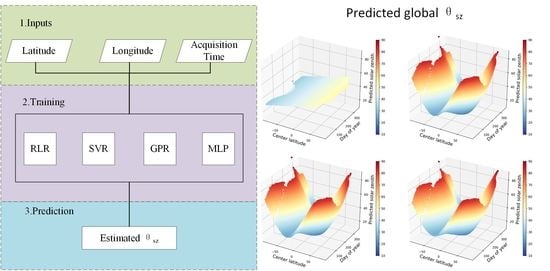
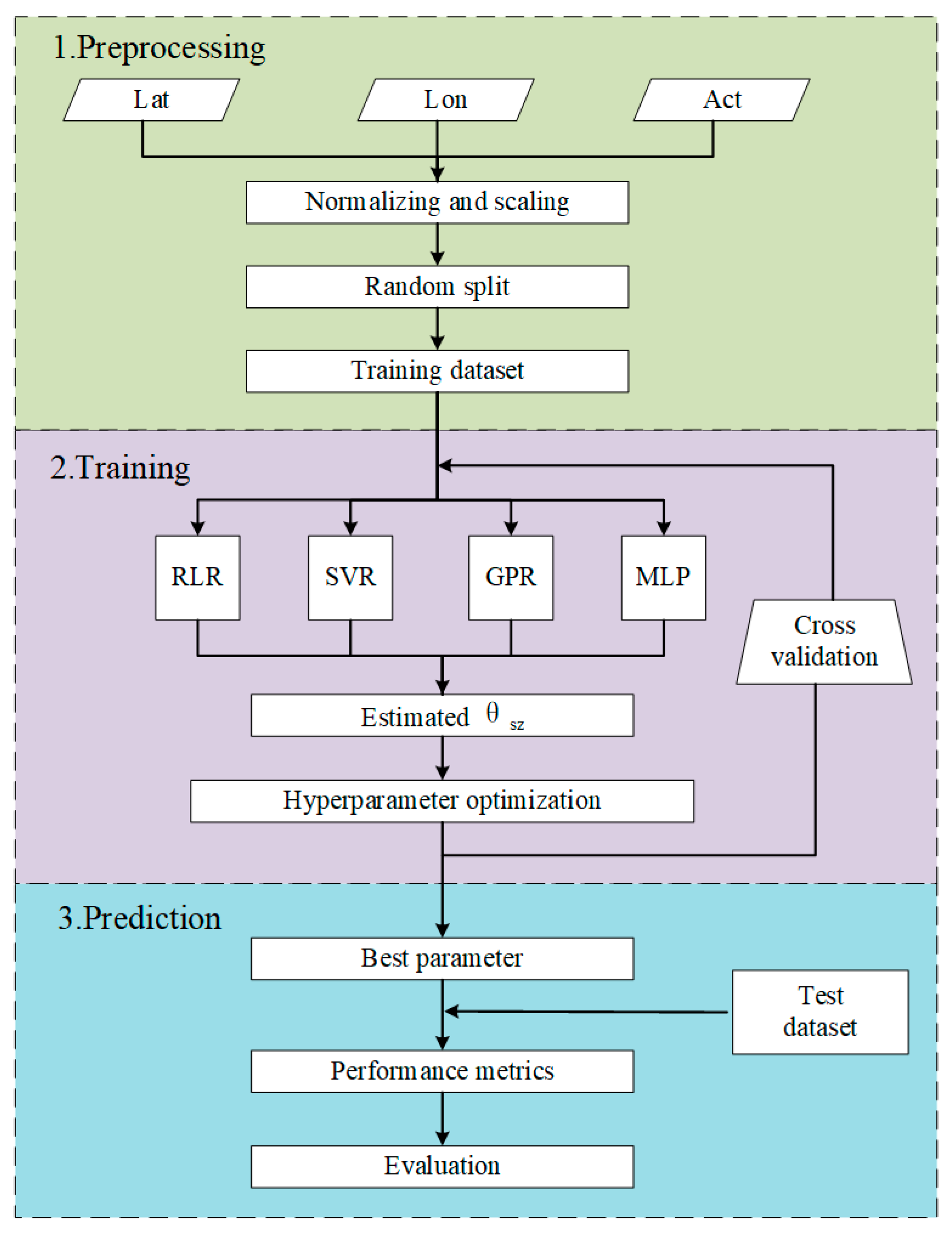
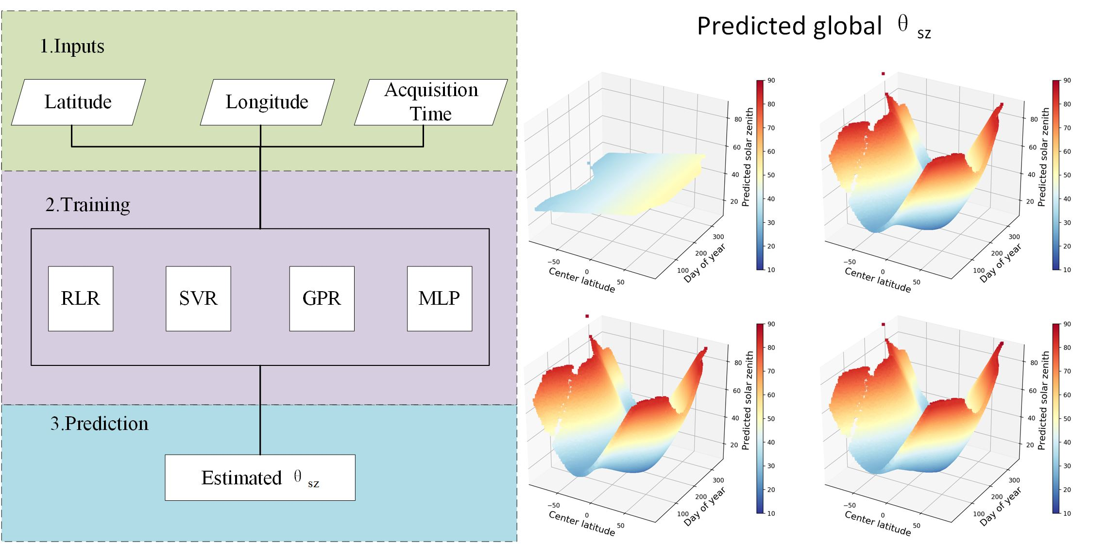
3. Methodology
3.1. Polynomial Regression Model
3.2. ML Regression Models
3.2.1. Regularized Linear Regression
3.2.2. Support Vector Regression
3.2.3. Gaussian Process Regression
3.2.4. Multi-Layer Perception
4. Results
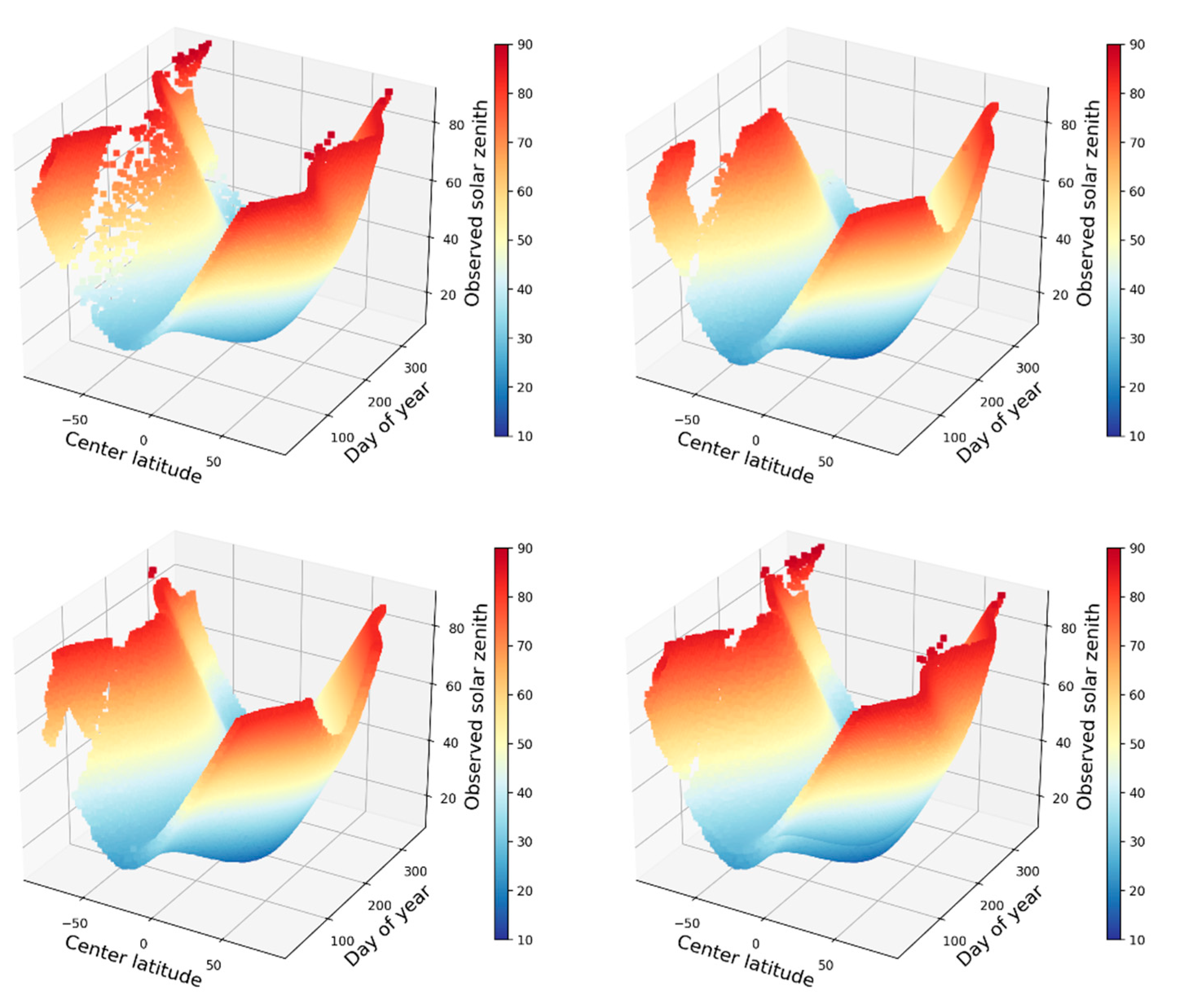
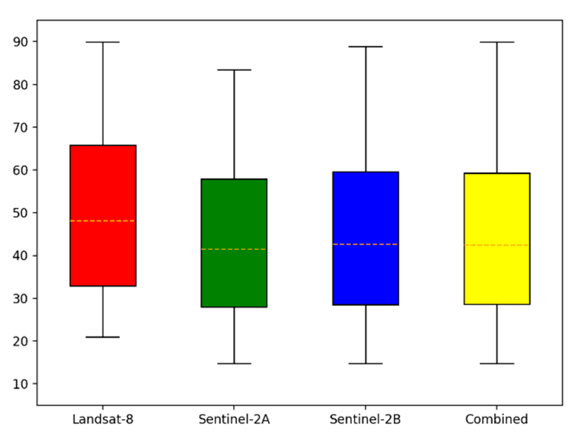
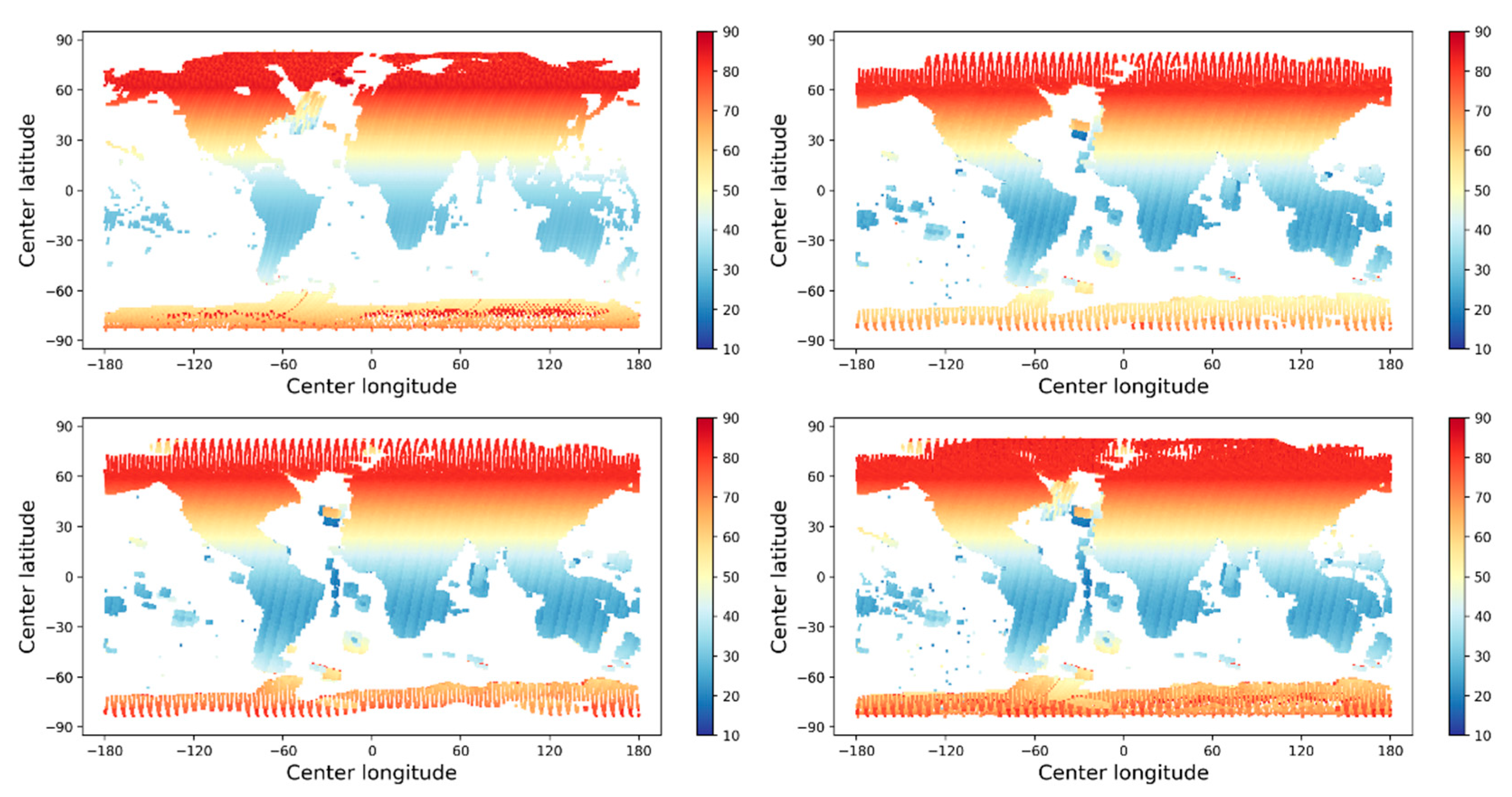
4.1. Global Distribution and Variations for Landsat-8 and Sentinel-2A/2B
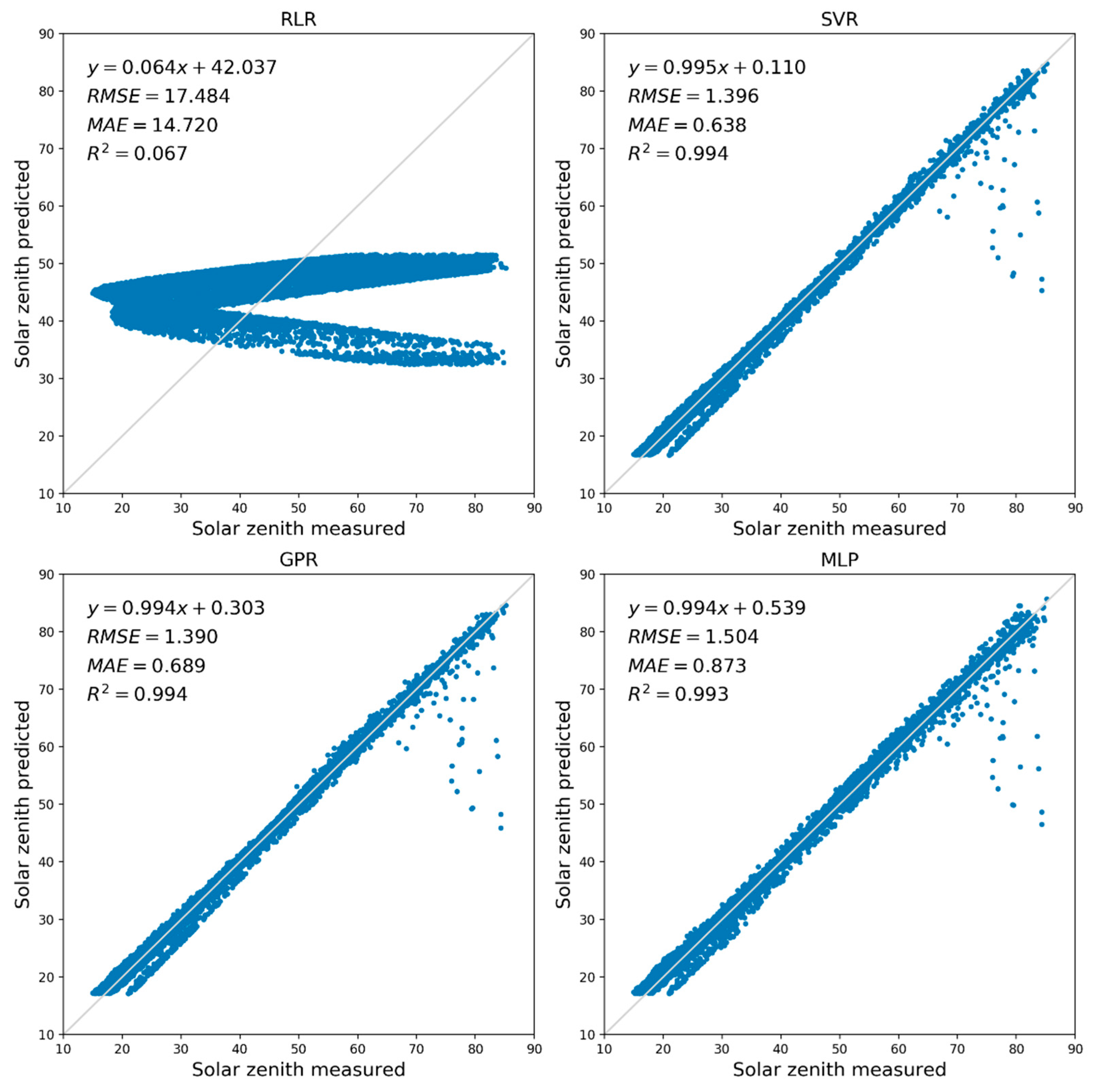
4.2. Performance of ML Models for Global Prediction
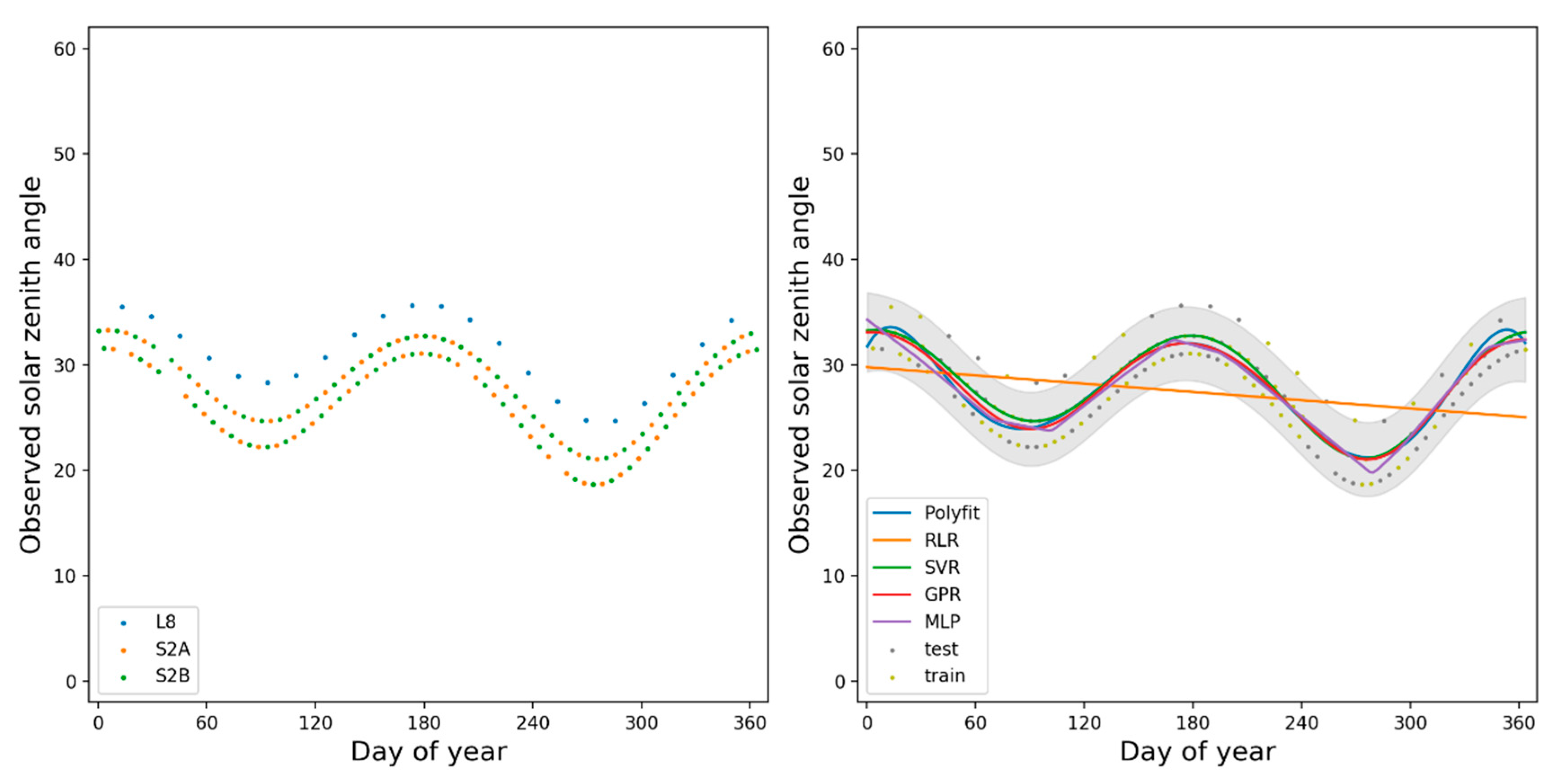
4.3. Performance of ML Models for Local Prediction
5. Discussion
6. Conclusions
Author Contributions
Funding
Institutional Review Board Statement
Informed Consent Statement
Data Availability Statement
Acknowledgments
Conflicts of Interest
References
- Knight, E.J.; Kvaran, G. Landsat-8 operational land imager design, characterization and performance. Remote Sens. 2014, 6, 10286–10305. [Google Scholar] [CrossRef] [Green Version]
- Loveland, T.R.; Irons, J.R. Landsat 8: The plans, the reality, and the legacy. Remote Sens. Environ. 2016, 185, 1–6. [Google Scholar] [CrossRef] [Green Version]
- Drusch, M.; Del Bello, U.; Carlier, S.; Colin, O.; Fernandez, V.; Gascon, F.; Hoersch, B.; Isola, C.; Laberinti, P.; Martimort, P. Sentinel-2: ESA’s optical high-resolution mission for GMES operational services. Remote Sensing Environ. 2012, 120, 25–36. [Google Scholar] [CrossRef]
- Li, J.; Roy, D.P. A Global Analysis of Sentinel-2A, Sentinel-2B and Landsat-8 Data Revisit Intervals and Implications for Terrestrial Monitoring. Remote Sens. 2017, 9, 9. [Google Scholar]
- Li, J.; Chen, B. Global Revisit Interval Analysis of Landsat-8–9 and Sentinel-2A-2B Data for Terrestrial Monitoring. Sensors 2020, 20, 6631. [Google Scholar] [CrossRef]
- Poortinga, A.; Tenneson, K.; Shapiro, A.; Nquyen, Q.; San Aung, K.; Chishtie, F.; Saah, D. Mapping plantations in Myanmar by fusing landsat-8, sentinel-2 and sentinel-1 data along with systematic error quantification. Remote Sens. 2019, 11, 831. [Google Scholar] [CrossRef] [Green Version]
- Roy, D.P.; Huang, H.; Boschetti, L.; Giglio, L.; Yan, L.; Zhang, H.H.; Li, Z. Landsat-8 and Sentinel-2 burned area mapping-A combined sensor multi-temporal change detection approach. Remote Sens. Environ. 2019, 231, 111254. [Google Scholar] [CrossRef]
- Veloso, A.; Mermoz, S.; Bouvet, A.; Le Toan, T.; Planells, M.; Dejoux, J.F.; Ceschia, E. Understanding the temporal behavior of crops using Sentinel-1 and Sentinel-2-like data for agricultural applications. Remote Sens. Environ. 2017, 199, 415–426. [Google Scholar] [CrossRef]
- Derkacheva, A.; Mouginot, J.; Millan, R.; Maier, N.; Gillet-Chaulet, F. Data Reduction Using Statistical and Regression Approaches for Ice Velocity Derived by Landsat-8, Sentinel-1 and Sentinel-2. Remote Sens. 2020, 12, 1935. [Google Scholar] [CrossRef]
- Roy, D.P.; Li, J.; Zhang, H.K.; Yan, L.; Huang, H.; Li, Z. Examination of Sentinel-2A multi-spectral instrument (MSI) reflectance anisotropy and the suitability of a general method to normalize MSI reflectance to nadir BRDF adjusted reflectance. Remote Sens. Environ. 2017, 199, 25–38. [Google Scholar] [CrossRef]
- Lucht, W.; Lewis, P. Theoretical noise sensitivity of BRDF and albedo retrieval from the EOS-MODIS and MISR sensors with respect to angular sampling. Int. J. Remote Sens. 2000, 21, 81–98. [Google Scholar] [CrossRef]
- Zhang, H.K.; Roy, D.P.; Kovalskyy, V. Optimal Solar Geometry Definition for Global Long-Term Landsat Time-Series Bidirectional Reflectance Normalization. IEEE Trans. Geosci. Remote Sens. 2016, 54, 1410–1418. [Google Scholar] [CrossRef]
- Claverie, M.; Ju, J.; Masek, J.G.; Dungan, J.L.; Vermote, E.F.; Roger, J.C.; Justice, C. The Harmonized Landsat and Sentinel-2 surface reflectance data set. Remote Sens. Environ. 2018, 219, 145–161. [Google Scholar] [CrossRef]
- Ruescas, A.B.; Hieronymi, M.; Mateo-Garcia, G.; Koponen, S.; Kallio, K.; Camps-Valls, G. Machine learning regression approaches for colored dissolved organic matter (CDOM) retrieval with S2-MSI and S3-OLCI simulated data. Remote Sens. 2018, 10, 786. [Google Scholar] [CrossRef] [Green Version]
- Shen, H.; Jiang, Y.; Li, T.; Cheng, Q.; Zeng, C.; Zhang, L. Deep learning-based air temperature mapping by fusing remote sensing, station, simulation and socioeconomic data. Remote Sens. Environ. 2020, 240, 111692. [Google Scholar] [CrossRef] [Green Version]
- Irons, J.R.; Dwyer, J.L.; Barsi, J.A. The next Landsat satellite: The Landsat data continuity mission. Remote Sens. Environ. 2012, 122, 11–21. [Google Scholar] [CrossRef] [Green Version]
- Gascon, F.; Bouzinac, C.; Thepaut, O.; Jung, M.; Francesconi, B.; Louis, J.; Fernandez, V. Copernicus Sentinel-2A Calibration and Products Validation Status. Remote Sens. 2017, 9, 584. [Google Scholar] [CrossRef] [Green Version]
- WWW1. Landsat Metadata. Available online: http://landsat.usgs.gov/consumer.php (accessed on 8 June 2019).
- USGS, Landsat Collection-1 Product Definition. Available online: https://www.usgs.gov/media/files/landsat-collection-1-level-1-product-definition (accessed on 16 April 2019).
- WWW2. Sentinel-2 Metadata. Available online: https://earthexplorer.usgs.gov (accessed on 8 June 2019).
- Roy, D.P.; Li, J.; Zhang, H.K.; Yan, L. Best practices for the reprojection and resampling of Sentinel-2 Multi Spectral Instrument Level 1C data. Remote Sens. Lett. 2016, 7, 1023–1032. [Google Scholar] [CrossRef]
- Camps-Valls, G.; Verrelst, J.; Munoz-Mari, J.; Laparra, V.; Mateo-Jiménez, F.; Gómez-Dans, J. A survey on Gaussian processes for earth-observation data analysis: A comprehensive investigation. IEEE Geosci. Remote Sens. Mag. 2016, 4, 58–78. [Google Scholar] [CrossRef] [Green Version]
- Liu, H.; Ong, Y.S.; Shen, X.; Cai, J. When Gaussian process meets big data: A review of scalable GPs. IEEE Trans. Neural Netw. Learn. Syst. 2020, 31, 4405–4423. [Google Scholar] [CrossRef] [Green Version]
- Roy, D.P.; Ju, J.; Kline, K.; Scaramuzza, P.L.; Kovalskyy, V.; Hansen, M.; Zhang, C. Web-enabled Landsat Data (WELD): Landsat ETM+ composited mosaics of the conterminous United States. Remote Sens. Environ. 2010, 114, 35–49. [Google Scholar] [CrossRef]
- Bengio, Y.; Grandvalet, Y. No unbiased estimator of the variance of k-fold cross-validation. J. Mach. Learn. Res. 2004, 5, 1089–1105. [Google Scholar]
- Lee, Y.; Han, D.; Ahn, M.H.; Im, J.; Lee, S.J. Retrieval of total precipitable water from Himawari-8 AHI data: A comparison of random forest, extreme gradient boosting, and deep neural network. Remote Sens. 2019, 11, 1741. [Google Scholar] [CrossRef] [Green Version]
- Maimaitijiang, M.; Sagan, V.; Sidike, P.; Hartling, S.; Esposito, F.; Fritschi, F.B. Soybean yield prediction from UAV using multimodal data fusion and deep learning. Remote Sens. Environ. 2020, 237, 111599. [Google Scholar] [CrossRef]
- Verrelst, J.; Muñoz, J.; Alonso, L.; Delegido, J.; Rivera, J.P.; Camps-Valls, G.; Moreno, J. Machine learning regression algorithms for biophysical parameter retrieval: Opportunities for Sentinel-2 and-3. Remote Sens. Environ. 2012, 118, 127–139. [Google Scholar] [CrossRef]
- Fernández-Delgado, M.; Cernadas, E.; Barro, S.; Amorim, D. Do we need hundreds of classifiers to solve real world classification problems? J. Mach. Learn. Res. 2014, 15, 3133–3181. [Google Scholar]
- Li, C.; Wang, J.; Wang, L.; Hu, L.; Gong, P. Comparison of classification algorithms and training sample sizes in urban land classification with Landsat thematic mapper imagery. Remote Sens. 2014, 6, 964–983. [Google Scholar] [CrossRef] [Green Version]
- Qian, Y.; Zhou, W.; Yan, J.; Li, W.; Han, L. Comparing machine learning classifiers for object-based land cover classification using very high resolution imagery. Remote Sens. 2015, 7, 153–168. [Google Scholar] [CrossRef]
- Brereton, R.G.; Lloyd, G.R. Support vector machines for classification and regression. Analyst 2010, 35, 230–267. [Google Scholar] [CrossRef]
- Deka, P.C. Support vector machine applications in the field of hydrology: A review. Appl. Soft Comput. 2014, 19, 372–386. [Google Scholar]
- Pedregosa, F.; Varoquaux, G.; Gramfort, A.; Michel, V.; Thirion, B.; Grisel, O.; Duchesnay, E. Scikit-learn: Machine learning in Python. J. Mach. Learn. Res. 2011, 12, 2825–2830. [Google Scholar]
- Chang, C.C.; Lin, C.J. LIBSVM: A library for support vector machines. ACM Trans. Intell. Syst. Technol. 2011, 2, 1–27. [Google Scholar] [CrossRef]
- Rasmussen, C.E.; Nickisch, H. Gaussian processes for machine learning (GPML) toolbox. J. Mach. Learn. Res. 2010, 11, 3011–3015. [Google Scholar]
- Verrelst, J.; Camps-Valls, G.; Muñoz-Marí, J.; Rivera, J.P.; Veroustraete, F.; Clevers, J.G.; Moreno, J. Optical remote sensing and the retrieval of terrestrial vegetation bio-geophysical properties–A review. ISPRS J. Photogramm. Remote Sens. 2015, 108, 273–290. [Google Scholar] [CrossRef]
- Verrelst, J.; Alonso, L.; Camps-Valls, G.; Delegido, J.; Moreno, J. Retrieval of vegetation biophysical parameters using Gaussian process techniques. IEEE Trans. Geosci. Remote Sens. 2011, 50, 1832–1843. [Google Scholar] [CrossRef]
- Morales-Alvarez, P.; Pérez-Suay, A.; Molina, R.; Camps-Valls, G. Remote sensing image classification with large-scale Gaussian processes. IEEE Trans. GeoScience Remote Sens. 2017, 56, 1103–1114. [Google Scholar] [CrossRef] [Green Version]
- Hecht-Nielsen, R. Theory of the backpropagation neural network. In Neural Networks for Perception; Academic Press: Cambridge, MA, USA, 1992; pp. 65–93. [Google Scholar]
- Wulder, M.A.; White, J.C.; Loveland, T.R.; Woodcock, C.E.; Belward, A.S.; Cohen, W.B.; Fosnight, E.A.; Shaw, J.; Masek, J.G.; Roy, D.P. The global Landsat archive: Status, consolidation, and direction. Remote Sens. Environ. 2016, 185, 271–283. [Google Scholar] [CrossRef] [Green Version]
- ED Chaves, M.; CA Picoli, M.; D Sanches, I. Recent Applications of Landsat 8/OLI and Sentinel-2/MSI for Land Use and Land Cover Mapping: A Systematic Review. Remote Sens. 2020, 12, 3062. [Google Scholar] [CrossRef]
- Gao, F.; He, T.; Masek, J.G.; Shuai, Y.; Schaaf, C.B.; Wang, Z. Angular effects and correction for medium resolution sensors to support crop monitoring. IEEE J. Sel. Top. Appl. Earth Obs. Remote Sens. 2014, 7, 4480–4489. [Google Scholar] [CrossRef]
- LeCun, Y.; Bengio, Y.; Hinton, G. Deep learning. Nature 2015, 521, 436–444. [Google Scholar] [CrossRef]
- Schmidhuber, J. Deep learning in neural networks: An overview. Neural Netw. 2015, 61, 85–117. [Google Scholar] [CrossRef] [PubMed] [Green Version]
- Masek, J.G.; Wulder, M.A.; Markham, B.; McCorkel, J.; Crawford, C.J.; Storey, J.; Jenstrom, D.T. Landsat 9: Empowering open science and applications through continuity. Remote Sens. Environ. 2020, 248, 111968. [Google Scholar] [CrossRef]


| Mean | Median | Standard Deviation | Maximum | Minimum | |
|---|---|---|---|---|---|
| Landsat-8 | 49.973° | 48.145° | 18.581° | 89.985° | 20.963° |
| Sentinel-2A | 43.890° | 41.573° | 17.951° | 83.377° | 14.739° |
| Sentinel-2B | 44.885° | 42.665° | 18.346° | 88.872° | 14.759° |
| Three sensors combined | 44.802° | 42.520° | 18.250° | 89.985° | 14.739° |
| Input | Metric | Polyfit | RLR | SVR | GPR | MLP |
|---|---|---|---|---|---|---|
| Lat | MAE RMSE | 0.525 10.597° 12.473° | 0.067 14.720° 17.484° | 0.516 10.581° 12.597° | 0.526 10.590° 12.463° | 0.525 10.619° 12.470° |
| Act | MAE RMSE | 0.114 14.633° 17.038° | 0.000 15.512° 18.101° | 0.113 14.593° 17.044° | 0.116 14.620° 17.023° | 0.113 14.635° 17.048° |
| Lat and Act | MAE RMSE | - | 0.067 14.720° 17.484° | 0.994 0.638° 1.396° | 0.994 0.689° 1.390° | 0.993 0.873° 1.504° |
| Lat and Lon and Act | MAE RMSE | - | 0.070 14.692° 17.454° | 0.993 0.711° 1.489° | 0.994 0.691° 1.391° | 0.992 1.052° 1.598° |
| Model | Time(s) | RAM(MB) |
|---|---|---|
| RLR | 1.36 | 501.7 |
| SVM | 7090.03 | 4999.9 |
| GPR | 1747.27 | 5118.5 |
| MLP | 2152.50 | 3512.2 |
| Metric | Polyfit | RLR | SVR | GPR | MLP | |
|---|---|---|---|---|---|---|
| Act | MAE RMSE | 0.778 1.550° 1.943° | −0.068 3.575° 4.263° | 0.816 1.334° 1.769° | 0.808 1.401° 1.810° | 0.784 1.520° 1.918° |
| Lat and Act | MAE RMSE | - | 0.036 3.508° 4.051° | 0.904 0.974° 1.279° | 0.943 0.907° 0.987° | 0.902 1.129° 1.294° |
| Lat and Lon and Act | MAE RMSE | - | 0.020 3.527° 4.084° | 0.753 1.464° 2.051° | 0.943 0.905° 0.986° | 0.851 1.291° 1.594° |
| Metric | Polyfit | RLR | SVR | GPR | MLP | |
|---|---|---|---|---|---|---|
| Act | MAE RMSE | 0.992 0.844° 1.228° | −0.104 13.059° 14.763° | 0.994 0.724° 1.099° | 0.993 0.790° 1.162° | 0.992 0.857° 1.240° |
| Lat and Act | MAE RMSE | - | −0.127 13.093° 14.920° | 0.997 0.625° 0.823° | 0.998 0.560° 0.632° | 0.993 0.972° 1.156° |
| Lat and Lon and Act | MAE RMSE | - | −0.144 13.183° 15.030° | 0.982 1.480° 1.899° | 0.998 0.543° 0.620° | 0.995 0.766° 0.991° |
| Metric | Polyfit | RLR | SVR | GPR | MLP | |
|---|---|---|---|---|---|---|
| Act | MAE RMSE | 1.000 0.164° 0.207° | −0.039 12.726° 14.443° | 1.000 0.153° 0.187° | 1.000 0.149° 0.181° | 1.000 0.183° 0.230° |
| Lat and Act | MAE RMSE | - | −0.034 12.677° 14.411° | 1.000 0.140° 0.185° | 1.000 0.125° 0.159° | 0.999 0.291° 0.351° |
| Lat and Lon and Act | MAE RMSE | - | −0.037 12.703° 14.429° | 0.991 0.994° 1.317° | 1.000 0.126° 0.165° | 0.999 0.238° 0.377° |
Publisher’s Note: MDPI stays neutral with regard to jurisdictional claims in published maps and institutional affiliations. |
© 2021 by the authors. Licensee MDPI, Basel, Switzerland. This article is an open access article distributed under the terms and conditions of the Creative Commons Attribution (CC BY) license (https://creativecommons.org/licenses/by/4.0/).
Share and Cite
Li, J.; Chen, B. Optimal Solar Zenith Angle Definition for Combined Landsat-8 and Sentinel-2A/2B Data Angular Normalization Using Machine Learning Methods. Remote Sens. 2021, 13, 2598. https://doi.org/10.3390/rs13132598
Li J, Chen B. Optimal Solar Zenith Angle Definition for Combined Landsat-8 and Sentinel-2A/2B Data Angular Normalization Using Machine Learning Methods. Remote Sensing. 2021; 13(13):2598. https://doi.org/10.3390/rs13132598
Chicago/Turabian StyleLi, Jian, and Baozhang Chen. 2021. "Optimal Solar Zenith Angle Definition for Combined Landsat-8 and Sentinel-2A/2B Data Angular Normalization Using Machine Learning Methods" Remote Sensing 13, no. 13: 2598. https://doi.org/10.3390/rs13132598
APA StyleLi, J., & Chen, B. (2021). Optimal Solar Zenith Angle Definition for Combined Landsat-8 and Sentinel-2A/2B Data Angular Normalization Using Machine Learning Methods. Remote Sensing, 13(13), 2598. https://doi.org/10.3390/rs13132598