Comparison of Random Forest, Support Vector Machines, and Neural Networks for Post-Disaster Forest Species Mapping of the Krkonoše/Karkonosze Transboundary Biosphere Reserve

Abstract

Mountain forests are exposed to extreme conditions (e.g., strong winds and intense solar radiation) and various types of damage by insects such as bark beetles, which makes them very sensitive to climatic changes. Therefore, continuous monitoring is crucial, and remote-sensing techniques allow the monitoring of transboundary areas where a common policy is needed to protect and monitor the environment. In this study, we used Sentinel-2 and Landsat 8 open data to assess the forest stands classification of the UNESCO Krkonoše/Karkonosze Transboundary Biosphere Reserve, which is undergoing dynamic changes in recovering woodland vegetation due to an ecological disaster that led to damage and death of a large portion of the forests. Currently, in this protected area, dry big trunks and branches coexist with naturally occurring young forests. This heterogeneity generates mixes, which hinders the automation of classification. Thus, we used three machine learning algorithms—Random Forest (RF), Support Vector Machine (SVM), and Artificial Neural Network (ANN)—to classify dominant tree species (birch, beech, larch and spruce). The best results were obtained for the SVM RBF classifier, which offered an average median F1-score that oscillated around 67.2–91.5% depending on the species. The obtained maps, which were based on multispectral satellite images, were also compared with classifications made for the same area on the basis of hyperspectral APEX imagery (288 spectral bands with three-meter resolution), indicating high convergence in the recognition of woody species.

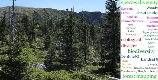
1. Introduction

Human activities have changed the environment for thousands of years. The significant increase in the population has resulted in increased socioeconomic activities associated with the production and consumption of environmental components. The pressure on ecosystems, natural habitats, and biodiversity loss are among the most intense impacts on the natural environment, and these effects translate into changes in mountain forested areas [1]. Therefore, an updated quality thematic mapping system is necessary to allow better analysis and decision making in forest management. Changes in forests have become a significant driver of climate change, but at the same time, climate changes affect habitats; therefore, it is essential to continuously acquire long-term observation series. Although costs of flight campaigns have decreased in recent years and their use has become more popular, the cost may be still too high for permanent monitoring. For this reason, attention is often paid to the use of free-of-charge satellite data, which has become a key element of environmental monitoring of large areas and for the protection of biodiversity [2,3]. One of the most popular types of data comes from the Landsat and Sentinel series satellites, which are commonly used to monitor different forest types and allow the identification of up to a dozen tree species [4,5,6,7]. Moreover, such techniques reduce the cost of intensive field work and, in some cases, are a good substitute for airborne images. Additionally, multitemporal data distinguishes species diversity in different periods of plant phenological development [8,9], allowing less frequent or more expensive data to be simulated, which can be used to monitor the condition of plants [10,11,12,13], including the early detection of bark beetle outbreaks in trees (starting from preliminary stages (green phase) up to dry trunks), which is a serious challenge for European managed forests [14]. The results obtained from Landsat and Sentinel-2 images differ from each other based on differences in the purpose of the work (identification of forest types or individual species), the additional data sources available (e.g., digital surface model [15], microwave data), as well as the specificity of the research area, the combination of scenes from different growing seasons [16,17,18], remote sensing vegetation indices [19,20,21], and adopted algorithms [22,23].

Currently, the most commonly used classifiers are based on nonparametric methods [24], e.g., artificial neural networks, which require significant computing resources, but offer good results [25]; the Support Vector Machine (SVM) [26,27,28]; and the Random Forest (RF) [29,30]. However, in large and homogeneous areas, parametric algorithms allow interesting results to be obtained [31]. Simple methods, e.g., the Maximum Likelihood, can be used to obtain the intended results. For example, Das and Singh [32] used Landsat TM (Thematic Mapper) data to identify four forest types with an overall accuracy of 85.1%. Noviar and Kartika [33] determined three tree classes with Landsat OLI (Operational Land Imager) images with an overall accuracy of 97%. Elhag [34] distinguished three tree species and two forest types with an accuracy of 98.1% using OLI images and showed that the most informative OLI channels were 3, 4, 5, 6, and 7. The most informative channel was 6, which is the short-wave infrared band (SWIR, 1570–1650 nm). Many authors have stated that, as classifiers, the SVM and RF algorithms offer high classification accuracy with a short computing time [35,36]. The Random Forest and Support Vector Machine are usually used for the classification of woody species, especially in multispectral data, due to the abovementioned reasons [37,38]. Banskota et al. [39] confirmed that the RF and SVM algorithms can be used to generate detailed maps, and the algorithms are characterized by easy processing.

A significant factor that contributes to accurate classification results is enrichment by multitemporal images and vegetation indices, which allows the overall accuracy to increase from 71% to 97% [22]. Using Landsat TM spring and fall scenes, Shao et al. [40] distinguished two tree species and two forest types with an accuracy of 89%. Similar observations were made by Zhu and Liu [16] who, using the Support Vector Machine algorithm, distinguished three forest classes with a total accuracy of 90.5%. Pasquarella et al. [41] used the Random Forest algorithm to identify eight forest types by testing different multitemporal datasets based on numerous images from different months. They achieved a producer accuracy (PA) ranging from 51% to 90%. Pena and Brenning [42], in addition to the standard Landsat OLI bands from spring, summer, and autumn, added the NDVI and NDWI. Then, based on the Random Forest algorithm, they identified three tree species with an overall accuracy of 94% and a producer accuracy in the range of 86% to 95%. Pimple et al. [43] tested the classification accuracy of three mountain forest types. The obtained results ranging from 78.4% to 82.3% (Landsat TM images) and from 81.0% to 82.3% (Landsat OLI). Using Decision Trees, Random Forest, and Support Vector Machine, Li et al. [31] separated three forest types on Landsat TM images, achieving an accuracy ranging from 79.1% to 88.2%, with Random Forest being the best algorithm and Decision Trees being the worst. Another example of the use of Sentinel 2 images and the Random Forest algorithm is the classification of six tree species found in the southern part of Germany [44]. The authors compared the difference in the accuracy of two classification methods: pixel and object-oriented. The overall accuracy was 66% for the object method and 63% for the pixel method.

The above examples show that woody forest species are characterized by a set of unique spectral features that can be identified using satellite images [45]. Additionally, the use of remote sensing vegetation indices and derivatives of altitude models allows both species and types of forests occurring in different biogeographic zones to be accurately identified. Of course, the best results are obtained for managed forests that cover dense, homogeneous areas, where the potential source of disturbance is quickly eliminated, creating optimal conditions for individual trees. This article focuses on semi-natural forests, such as mountain national parks and the UNESCO Biosphere Reserve, which, fifty years ago, was affected by major changes caused by acid rain, which disrupted not only leaves but also the soil, leading to destructive changes in the rhizosphere. The damaged trees largely remain in this protected area, which, according to legislation is now a living laboratory of natural processes. A new generation of trees grows intensively between the dry trunks, making it difficult to recognize the objects present there. Hence, the purpose of this article is to evaluate the methods that can be used to select representative pattern polygons for classification and verification of the obtained results. Then, we evaluate commonly available machine learning algorithms implemented in R programming language. For this, we use remote sensing methods to allow for the analysis of the entire park area. In terms of remote sensing, a detailed classification of six dominant tree species was carried out by Raczko and Zagajewski [46] using APEX aerial hyperspectral images and artificial neural networks, and an an overall accuracy of 87% was achieved, while a detailed analysis of non-forest areas was carried out by Marcinkowska-Ochtyra et al. [47], who achieved an overall accuracy of 84%, with fourteen out of twenty-four plant communities achieving a producer accuracy (PA) of more than 80% and sixteen out of twenty-four achieving an acceptable user accuracy (UA).

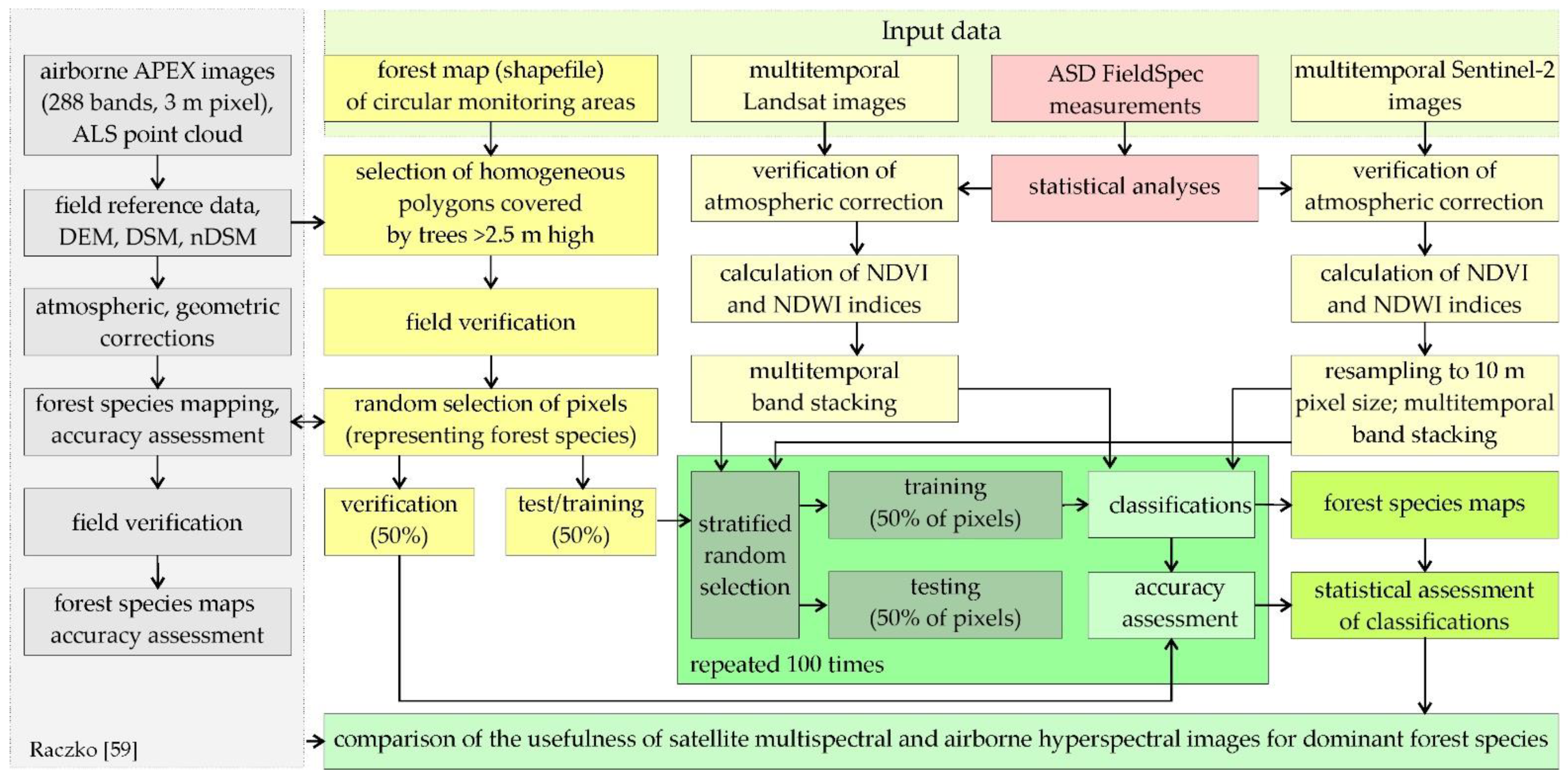
A motivation and a goal of the study was an assessment of remote sensing tools for mapping of transboundary diverse mountain area, which was affected by an ecological disaster 40 years ago. First rains, which were more acidic than lemon juice, weakened the photosynthetic apparatus and then the condition of plants and soil; it translated into on insect outbreaks leading to damages of the biosphere and rhizosphere. Plant recovery possibilities were very limited due to the status of the area (strictly protected area as national parks and as the UNESCO Biosphere Reserve) The consequences of the situation resulted in the fact that both dead tree trunks and spontaneously appearing different species of different ages appear next to bare rocks and exposed soil. This creates a huge mosaic of objects affecting the reflected electromagnetic signals. So, the intention of this manuscript was to use three well-known non-parametric classifiers, which proved their usefulness by different authors, offering good results. As reference data, maps achieved on the basis of the APEX airborne hyperspectral images, Airborne Lidar Scanning (ALS) and numerous field mapping were used. It allowed to obtain appropriate patterns for training and validation of the Landsat 8 and Sentinel-2 data-based classifications. The innovative element of the study is a verification of image classification algorithms of the mountain heterogeneous environment. The proposed solution allows a development of a monitoring system of the cross-border area, managed according to national environmental protection concepts (different statuses of individual protection zones). Additionally, an assessment of an impact of the size of training and verification patterns on the classification accuracies, which has a practical impact for the field campaign planning phase. To conclude this section, open, objective, and regularly repeatable satellite images and the open-source R programming language are good sources of information for large areas. The aim of the work is to assess different machine learning classification methods to classify the dominant species composition in the stand of the mountain forest, which is characterized by intensive dynamic growth due a previous ecological disaster that caused mass dieback of stands in the area of 15,000 ha [48].

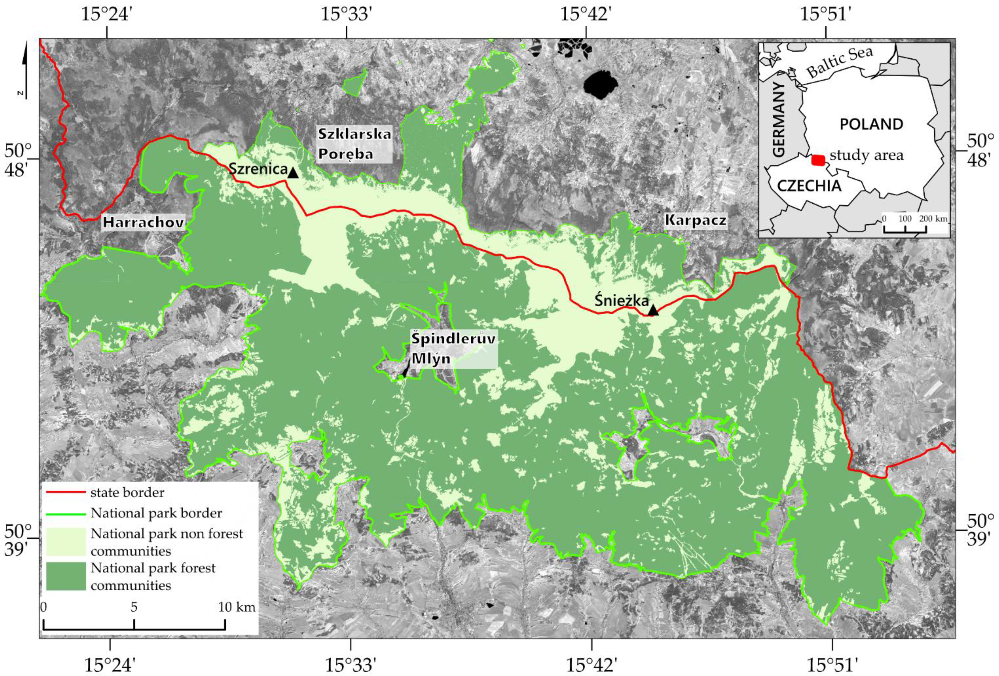
Research Area

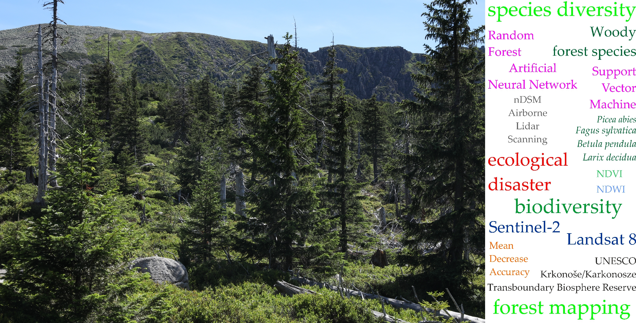
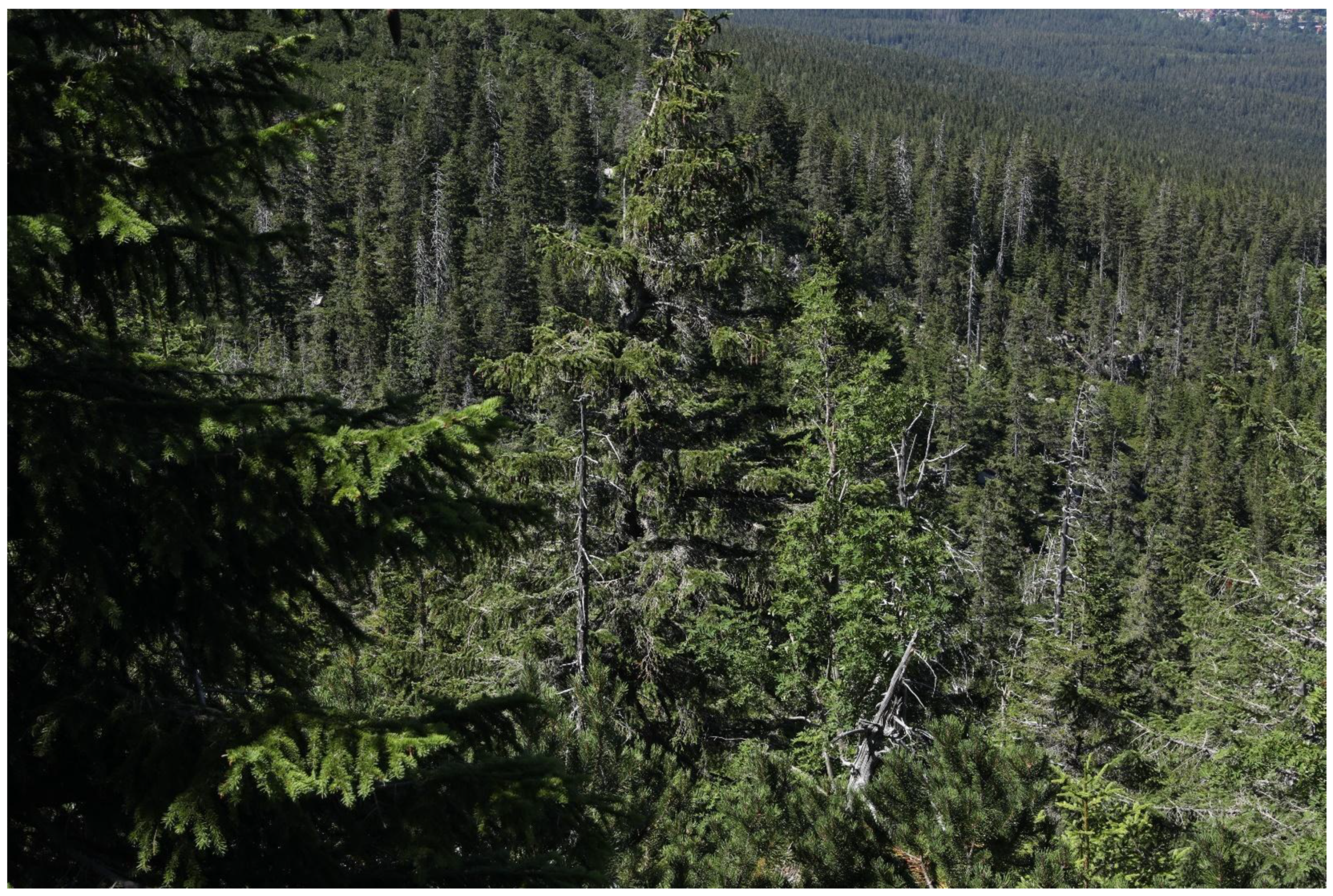
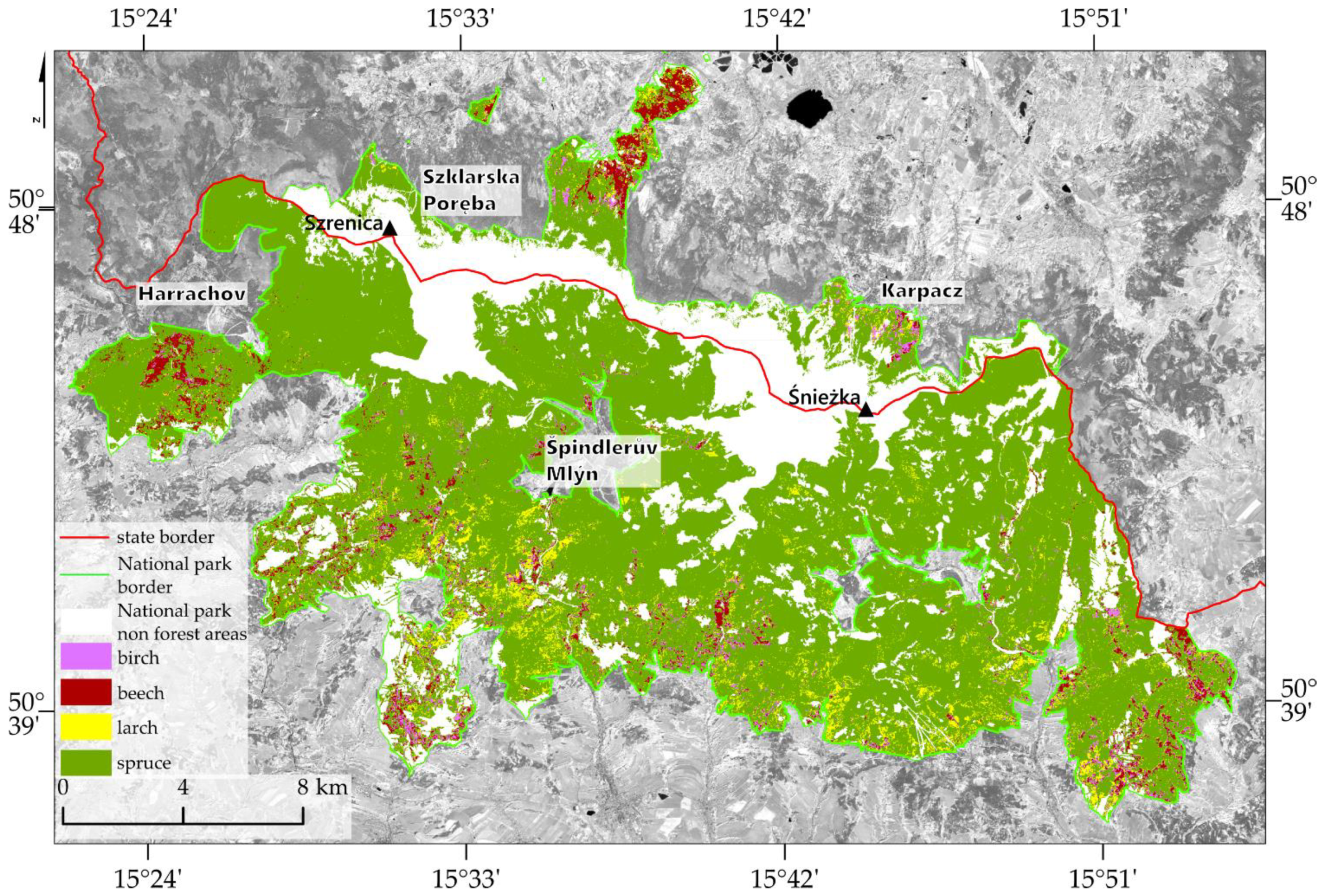
The Giant Mountains area was affected by an ecological disaster in the 1970s and 1980s [49,50]. Due to the synergistic actions of heavy air pollution, acid rains, strong winds, drought, and tree pest outbreaks, massive forest dieback, especially of spruce trees, and soil degradation occurred (Figure 1) [51]. However, the actions taken to regenerate the forest considered the proper species composition in consistency with potential habitats when trees were planted [52]. For this purpose, nest planting of originally occurring tree species was conducted, enabling the rebuilding of the species composition of the forest [53]. Numerous activities related to the reconstruction of forest ecosystems necessitated constant and objective monitoring of vegetation [54]. These efforts brought about expected results, which, in 1992, resulted in the establishment of the Transboundary UNESCO Biosphere Reserve.

The research area covers the Giant Mountains, extending over an area of approximately 38 km and a width of 8–20 km, covering approximately 650 km², of which approximately 28.5% belongs to Poland and the rest to the Czech Republic (Figure 2). The main part of the Mountains is located at the Czech–Polish border, the northern part is located in the Polish Karkonoski National Park (KNP), and the southern part is located in the Czech Krkonoše Mountains National Park (KRNAP).

The Karkonosze Mountains are quite rich and have an extensive hydrographic network [55]. Gusty and dry fen winds, which are formed when crossing a mountain barrier, are common and often cause damage to forest stands. The harsh conditions of the Karkonosze Mountains have shaped the characteristics of the existent plants. There are lower plant layers than in other Central European mountains [55]. In the primeval forest, the species with the largest shares in the composition are spruce (53%), beech (23%), and fir (11%) [56,57]. Currently, the dominant woody species is spruce (Picea abies L. Karst), and the remaining species that have significant shares are birch (Betula pendula Roth), beech (Fagus sylvatica L.), and larch (Larix decidua Mill).

2. Materials and Methods

A classification of woody species based on Sentinel-2 MSI and Landsat 8 OLI satellite images and field-verified polygons was conducted to identify representative patterns for the optimization of classifier parameters of Random Forest and Support Vector Machines. These algorithms were selected due to the ease of open-source implementation and the high accuracy of classification achieved (Figure 3) [58].

2.1. Satellite Input Data

Landsat satellite images for the following months in 2018 were obtained from the USGS Earth Explorer service (Path: 191 Row: 25) in GeoTIFF format: 20 April, 15 June, 30 October. Sentinel-2 images (level 2A) were acquired using the Copernicus Open Access Hub (acquired on 19 April, 7 August, 17 November in 2018;

Table 1. Characteristics of satellite data used for classification.

Satellite	Sentinel-2 (MSI)	Landsat 8 (OLI)
processing level	Level 2A	Level-2
scene location	granule: 33UWS	path: 191, row 25
resolution	10 m	30 m
dates	19 April 2018	20 April 2018
	7 August 2018	15 June 2018
	17 November 2018	30 October 2018

). Only scenes with less than 10% cloudiness were selected for further processing. The studied area is mountainous, so the choice of scenes was limited due to frequent cloud cover. Acquired Sentinel-2 and Landsat images were corrected atmospherically by ESA (level 2A) and USGS (Level-2). Nevertheless, due to the use of images from different periods and areas, the authors verified the atmospheric correction models based on Warsaw’s polygons and ASD FieldSpec 4 (with the ASD ContactProbe; Analytical Spectral Devices, Inc., Longmont, CO, USA). For this purpose, spectrometric measurements of 59 large, homogeneous, and dominant calibration targets (asphalt, concrete, gravel, and paving stones) in Warsaw and surrounding areas were made. The comparison between field measurements, six Sentinel-2 MSI, and three Landsat 8 OLI images indicated that the average Root Mean Square Error (RMSE) oscillated around 0.04−0.07 for the Sentinel-2 images and around 0.05−0.07 for Landsat images [58]. APEX (Airborne Prism EXperiment) airborne hyperspectral data acquisition with 288 bands (413−2440 nm) and a spatial resolution of 3.35 m was executed on 10 September 2012. APEX images allowed us to prepare a high-resolution woody species map, which was carefully field verified on many research transects [59], creating a reliable reference material for this study.

2.2. Field Data Collection

Due to its large size and difficult accessibility, the Karkonosze National Park manages stands based on a network of circular areas, which do not comprehensively cover the entire area of the Polish Park (Figure 4). The updated field patterns were used by Edwin Raczko [59] to generate a reference vector shapefile. This allowed the identification of homogenous polygons using the Lecia ZENO 10 GNSS receiver with an external antenna for geolocation. The measurement was based on the RTK (Real Time Kinematic) technique using the European Position Determination System (ASG-EUPOS). The Position Dilution of Precision (PDOP) values were less than 2, and the positioning accuracy was lower than 1 m. Field campaigns were conducted to collect data in the following years: 2014, 2015, and 2016. More than 1000 field measurements were collected during all campaigns, including within the park network. Then, these polygons were verified on the Normalized Digital Surface Model (nDSM, generated from the Airborne Lidar Scanning (ALS) point cloud obtained from the KNP). The data were processed in the LASTOOLS program, developed by the nDSM, which allowed the selection of homogeneous polygons representing tree species on reference plots (trees over 2.5 m high). This value was selected empirically for use to remove areas covered with low vegetation from the nDSM. The polygons belong to the network of circular polygons run by the Polish Karkonosze National Park. Due to the pixel sizes of the Landsat 8 OLI and Sentinel-2 data, the field-acquired data represent homogenous polygons of tree species on Sentinel-2 and Landsat 8 images [24,46]. In this study, we focused on four tree species that have dominant shares in the park’s stand structure: birch (Betula pendula Roth), beech (Fagus sylvatica L.), larch (Larix decidua Mill), and spruce (Picea abies L. Karst). Due to the pixel sizes of Sentinel-2 (100 m²) and Landsat (900 m²) data, it is impossible to identify rare species, which constitute 0.94% of the area [24]: alder (Alnus Mill.), Norway maple (Acer platanoides L.), and fir (Abies Mill.).

2.3. Satellite Data Processing

We used all Sentinel-2 spectral bands (10, 20 and 60 m), because we did not want to assume in advance that they might not contribute any information (and this hypothesis was confirmed). In the following step, pixels of 20 and 60 m bands were resampled to 10 m resolution to unify their size, and Landsat 8 images were kept at a resolution of 30 m. In order to distinguish between deciduous and coniferous species more precisely, satellite images from three vegetation periods (spring, summer and autumn) were used. In the next step, multi-temporal compositions were made separately for Sentinel-2 and Landsat 8 data as a layer stack. Based on the images remote-sensing vegetation indices were calculated (

Table 2. Used formulas to calculate the indices.

	NDVI	NDWI
General equation	(NIR − RED)/(NIR + RED)	(NIR − SWIR)/(NIR + SWIR)
Sentinel-2	(B8 − B4)/(B8 + B4)	(B3 − B8)/(B3 + B8)
Landsat 8	(B5 − B4)/(B5 + B4)	(B5 − B6)/(B5 + B6)

). Firstly, the Normalized Difference Vegetation Index (NDVI) [60] was used to show the general quantity and vigor of green plants. After the ecological disaster, the area was characterized by a large number of remaining dry trunks and branches, which significantly modified the spectral reflection, masking young trees that were intensively growing around dead trees. Thus, the Normalized Difference Water Index (NDWI) [61] was used to determine the canopy water content, which allowed us to identify healthy, deciduous, and coniferous trees by their water contents [20]. Both indices were calculated for all scenes to increase the classification accuracy of damaged plants [62]. Additionally, in the following stage, the indices were used to determine the masking of non-forest areas. Then, spectral bands and indices were stacked into separate GeoTiFF files for Sentinel-2 and Landsat 8 images. Then, pixel values were extracted from images based on polygons to obtain samples for classification (

Table 3. Size of the set used for classification.

Class	Number of Polygons	Number of Pixels S-2	Number of Pixels L8
Birch	108	252	105
Beech	109	243	128
Larch	144	324	124
Spruce	370	867	505

).

2.4. Classification and Accuracy Assessment

The classification was carried out using R 4.0.0 programming language in R Studio [63,64,65]. This was chosen due to the high availability of these software packages and the ease of implementation of the classifier training process and display classification. We used the Random Forest algorithm [29] from the randomForest package [66]. The parameters define ntree out of 500, because the OOB (out of bag) error values above this number usually stabilize [37]. Tuning was applied to the mtry parameter, and the mtry with the lowest OOB error value was selected. Random Forest was also used to obtain information on the variable importance impact of the classification accuracy, by using Mean Decrease Accuracy (MDA). This was performed for individual bands and indices from different time periods, which indicated how much accuracy the model suffers when each variable is excluded. As the accuracy loss increases, the more important the variable is for the classification.

To implement artificial neural networks, a multi-layer perceptron (MLP) was used from the nnet package [67]. With the grid search methods, hyperparameters (decay, hidden units) were optimized for a set of samples from Sentinel-2 and Landsat 8.

In the case of the Support Vector Machine algorithm [26], the e1071 package was used [68], which performs the standardization of spectral features in the svm function (additionally we used the tune function from the e1071 package, which performs cross-validation during the tuning process). The learning parameters were optimized using the grid search method, where each combination of parameters was checked from the pool of parameters. Tuning was performed for linear, polynomial, radial basis function kernel (RBF), and sigmoid kernel functions (

Table 4. Tested SVM hyperparameters.

Parameters	Kernel Function	Min.	Max.	Step	Scale
cost	linear, RBF, polynomial, sigmoid	0.001	10,000	10	logarithmic
gamma	RBF, polynomial, sigmoid	0.001	10,000	10	logarithmic
coef0	polynomial, sigmoid	0 (kept the default value)
degree	polynomial	3 (kept the default value)

). The tuning parameters were selected for kernels: gamma = 0.01, cost = 100.

The first step was to extract each class’s patterns from the image pixels using the raster and rgdal packages [69,70]. Then, on the obtained datasets, the algorithm training parameters were optimized, and tuning of all classifiers’ parameters was performed on its entire set of patterns. The parameter optimization procedures were performed on the references derived from the Multispectral Instrument Sentinel-2 (MSI) and Landsat 8 OLI images.

The influence of the number of pixels on the classification accuracy was also checked. The following pixel thresholds were investigated for each class: 50, 100, 150, 200, and 300. Due to the heterogeneity of the analyzed targets and based on previous experience [58], we focused on 300 pixels for each class in the training set and carried out an iterative accuracy assessment, which means that all classifications were repeated 100 times, according to the following steps:

• The random selection of reference pixels for the training and testing datasets in a ratio of 50:50 to meet the condition of independence [71]. The rngtools and doRNG packages were used to generate random seeds and optimize the execution time of the iterative accuracy assessment. The multiple cores of the processor utilized doParallel, and for each package that used a PSOCK (Parallel Socket Cluster), a cluster was used [72,73];
• The training of Random Forest and Support Vector Machine classifiers;
• The accuracy assessment of each classification;
• The classification accuracy results and a random seed were saved.

This approach allowed us to get more objective results because using one time split of samples between training and testing can be biased. The iterative accuracy assessment method, which was repeated one hundred times, showed the ranges of accuracy values that each class can achieve.

Then, the classification accuracy of the remaining areas was assessed on the algorithms’ selected parameters, where the parameters were found to be satisfactory in all cases. The following metrics were used to assess the classification accuracy [74]:

• Overall accuracy (OA)—the ratio of all correctly classified pixels to the sum of all pixels [75];
• User accuracy (UA)—the ratio of correctly classified pixels in a given class to all pixels classified as belonging to this class [76];
• Producer accuracy (PA)—the ratio of correctly classified pixels of a given class to all reference pixels of a given class;
• The Kappa coefficient was used to present the final results, but the index was characterized by having a high correlation with the overall accuracy, and thus the redundancy of information was doubled [77].
• F1-score—the weighted harmonic mean of the user and producer accuracy [78,79].

A confusion matrix was also used. This presented correctly classified pixels in its diagonal direction [74]. Box plots were also used. Then, the average accuracy levels showen by the F1-score coefficient values of the different classes were compared. For production of the final maps, models with the highest average F1-score for all scenario classes were selected.

3. Results

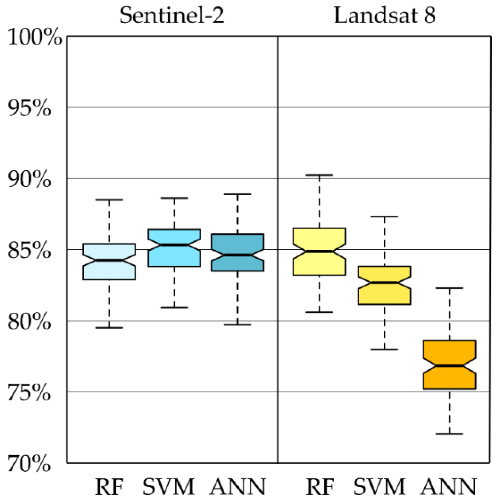
The results of the abovementioned activities included a map of dominant woody species present in 2018, classification accuracy measures in the form of error matrices, and box plots obtained with an iterative classification method using Landsat 8 and Sentinel-2 images. It should be emphasized that all classification approaches obtained similar results (Figure 5). The highest median from 100 iterations was obtained with Sentinel-2 images and the SVM algorithm (86%). A slightly lower median value was obtained for the Landsat 8 images and the Random Forest algorithm (85%). The Random Forest classifier gave a slightly lower value for Sentinel-2 images (84%).

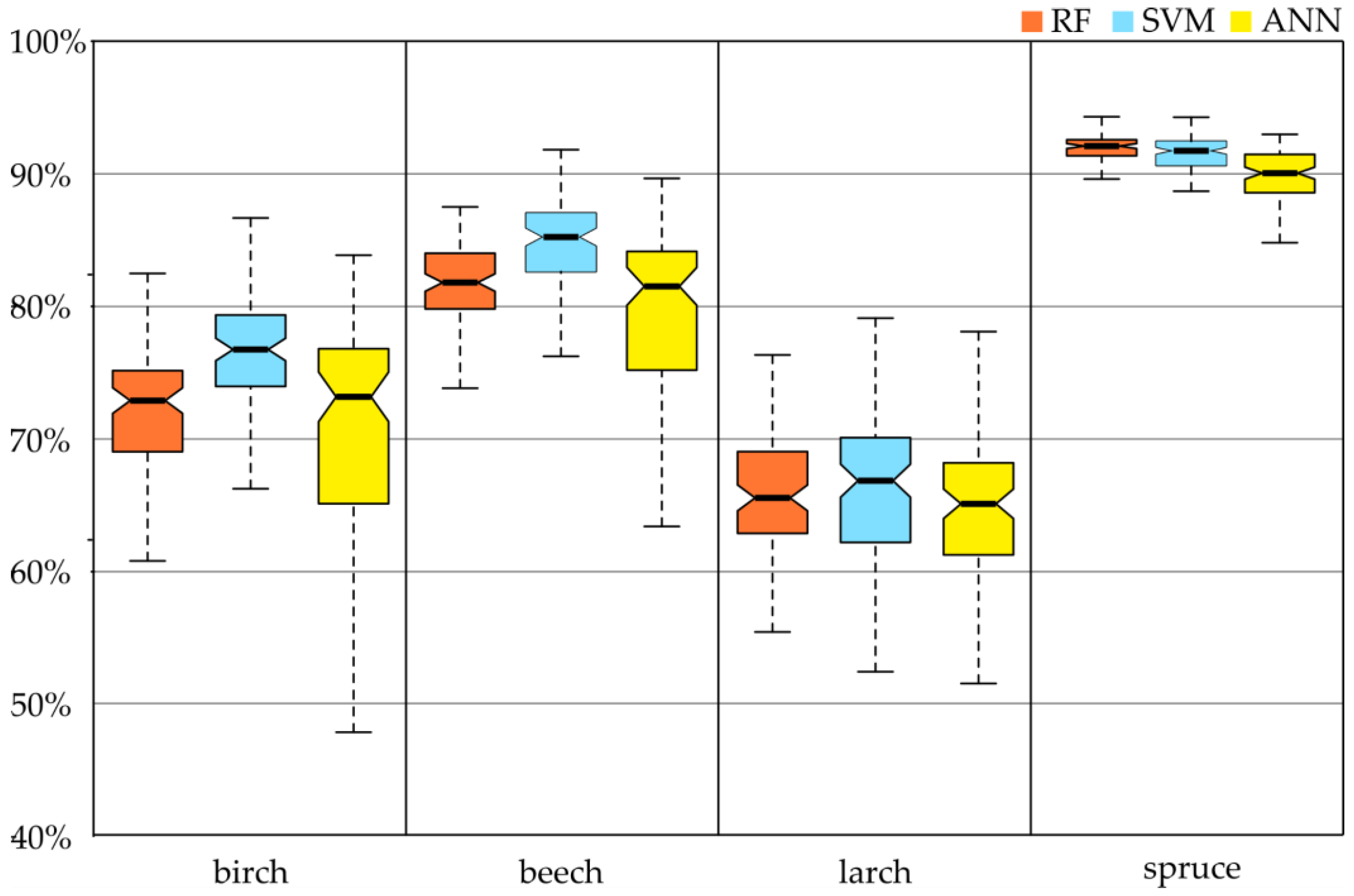
On the Sentinel-2 images, spruce was classified with the highest accuracy (regardless of the classifier, the F1-score oscillated around 90%; Figure 6). Slightly lower results were obtained for the beech class, especially with the SVM classifier (85%). For RF and ANN, the accuracy was about 82% (however, the spread of the results of individual iterations of ANN ranged from 64% to 89%). Similar outcomes occurred for the birch and larch.

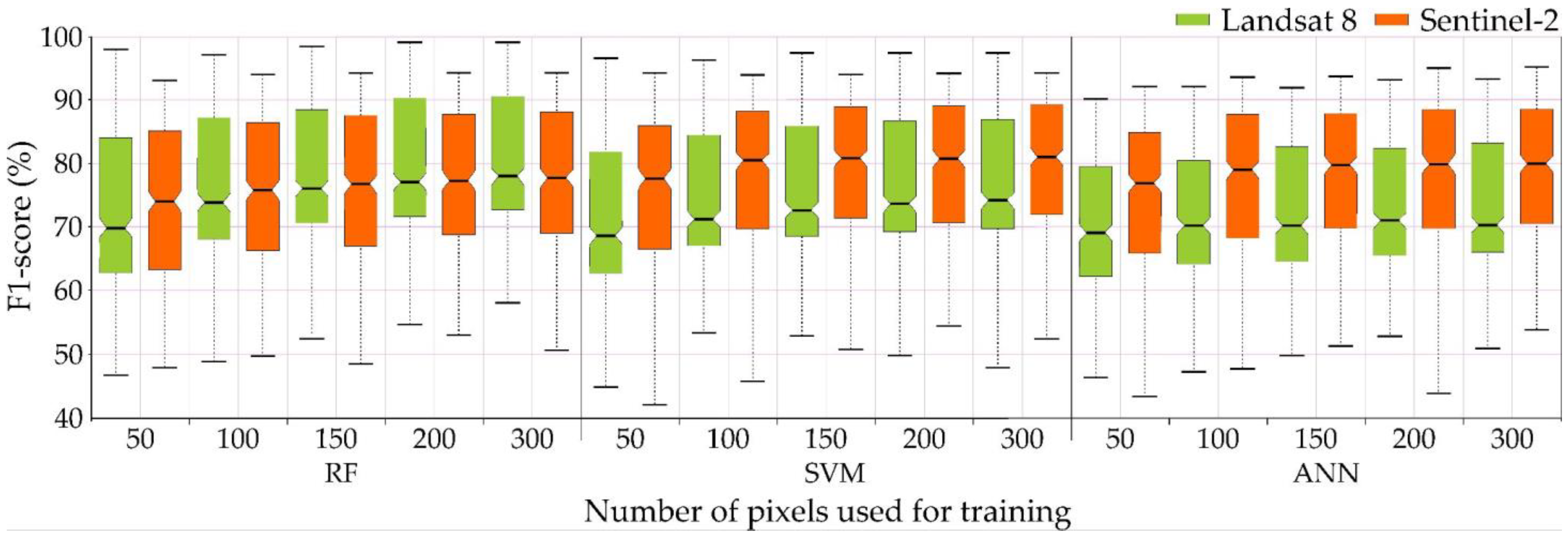
Landsat images allowed dominant woody species to be classified with a good overall accuracy (85% RF, 83% SVM RBF, Figure 7), but in the case of Sentinel-2 images, the SVM RBF classifier offered an overall accuracy of 87%, RF gave an accuracy of 83%, and ANN gave an accuracy of 84%, thus confirming their suitability for large-scale monitoring of the stand species composition. The Random Forest classifier offered the highest accuracy for tree species classification, followed by the SVM. Straightforward implementations of Artificial Neural Networks (such as Multi-layered Perceptron) seem to be insufficient for mapping tree species at resolutions offered by the Landsat and Sentinel 2 datasets. Further work should focus on the use of more sophisticated ANNs (e.g., deep artificial neural networks). For Landsat and Sentinel-2 images, the ranges of the first and third quartiles (Q1–Q3) were similar; however, the median values were about 5–9% higher for Sentinel-2 images (Figure 7). The detailed analysis of the impact of the number of pixels used in the training samples of all classifiers confirmed the high effectiveness of both SVM and RF. Furthermore, a median F1-score of 75−78% (median F1-score; Figure 7) was obtained with a relatively small sample (50 pixels), and the addition of more pixels to the training patterns allows an F1-score of about 80%. In the case of SVM, when there were 100−300 pixels in the pattern, the F1-score exceeded this value. Similar results were observed for analyses carried out on Landsat 8 data, but the median F1-score was lower by a few percentage points. In the case of Landsat 8, the best classifier was the Random Forest. In addition, the scatter of the results from individual iterations was significantly higher, because the best individual classifications allowed a score close to 100% to be obtained, while the lowest achieved scores below 50% (Figure 7). The results of the tree species classification performed on the multitemporal Sentinel-2 dataset are presented in

Table 5. Error matrix of the best results acquired based on Sentinel-2, Support Vector Machine classifier, and field verified polygons (Figure 8; OA = 86.5%, Kappa coefficient = 0.77; UA—User Accuracy, PA—Producer Accuracy, F1-score).

	Birch	Beech	Larch	Spruce	UA (%)	F1 (%)
birch	67	10	3	8	76.1	80.2
beech	7	86	1	2	89.6	86.0
larch	0	4	67	20	73.6	70.2
spruce	5	4	29	377	90.8	91.7
PA (%)	84.8	82.7	67.0	92.6

.

The Karkonosze forests are mainly dominated by spruce and also occupy the largest area on the map obtained (Figure 8). Deciduous species were also well distinguished. Beech was found to be the second most abundant species after spruce in the Czech Krkonoše forest stands, as can be seen on the map. The number of birch trees was found to be much lower and they occur sporadically, which can also be seen on the map. There was a slight overestimation of larch due to the fact that it was often planted as a protective belt for other species and mixed with their spectral reflectance. The overall accuracy result can be regarded as satisfactory (OA 86.5%). The analysis of the results showed that the broadleaved species had a smaller accuracy gap (F1-score: 80–86%) than the coniferous species (70–92%). The best level of accuracy was obtained for spruce (92%) and beech (86%). Slightly weaker but still good accuracy was obtained for birch (80%), while larch (70%) performed worse than other species, especially in terms of omission (PA 67%). Misclassification most often occurred due to the mixing of classes within the coniferous or deciduous communities, but the results should be considered satisfactory (Table 5).

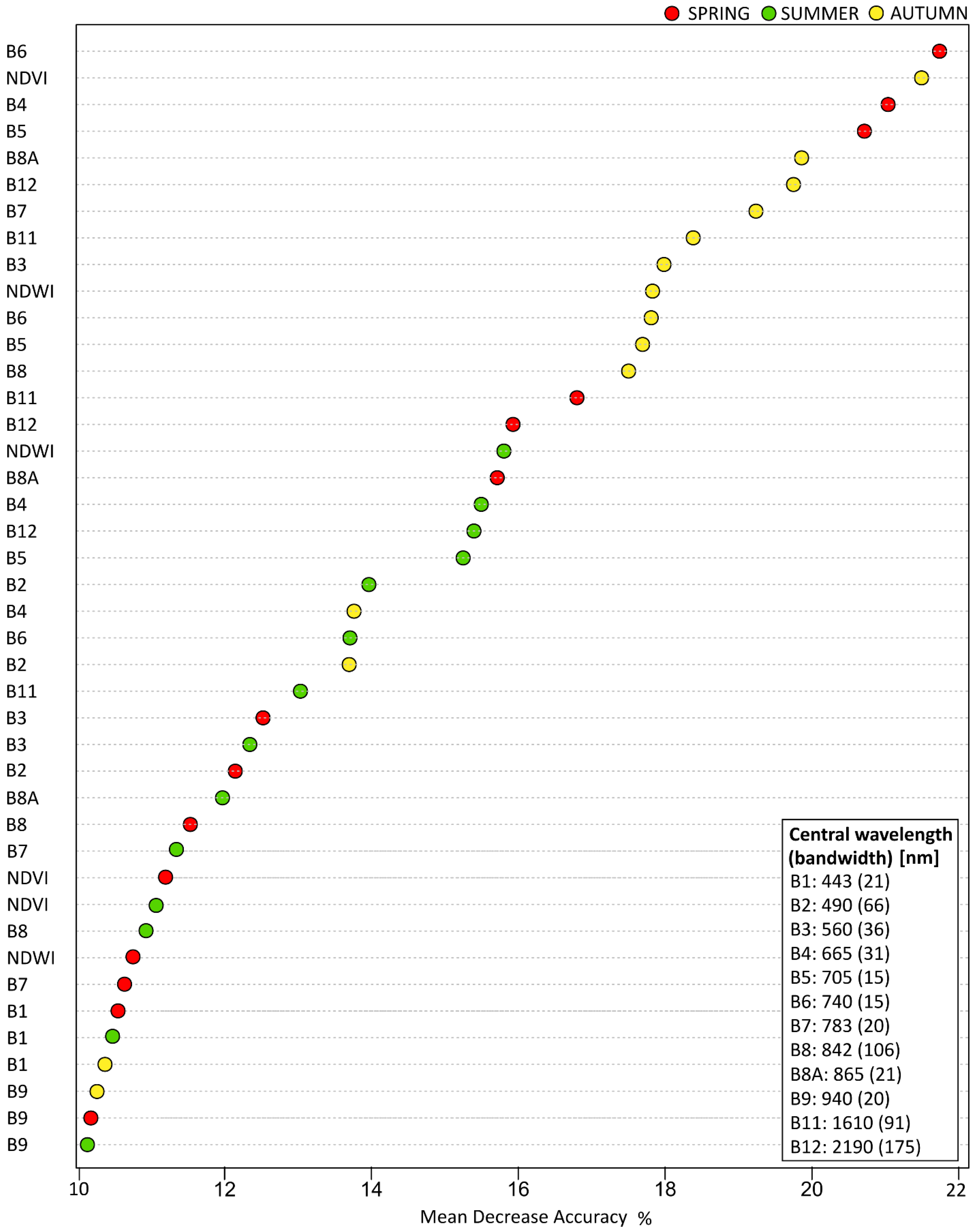
During the process of training Sentinel-2 images, the variable importance impact of the classification accuracy was tested, by using a mean decrease accuracy indicator. From the results (Figure 9), B6 (740.5 nm), NDVI, B4 (664.6 nm) and B5 (704.1 nm) were shown to be the most important variables.

4. Discussion

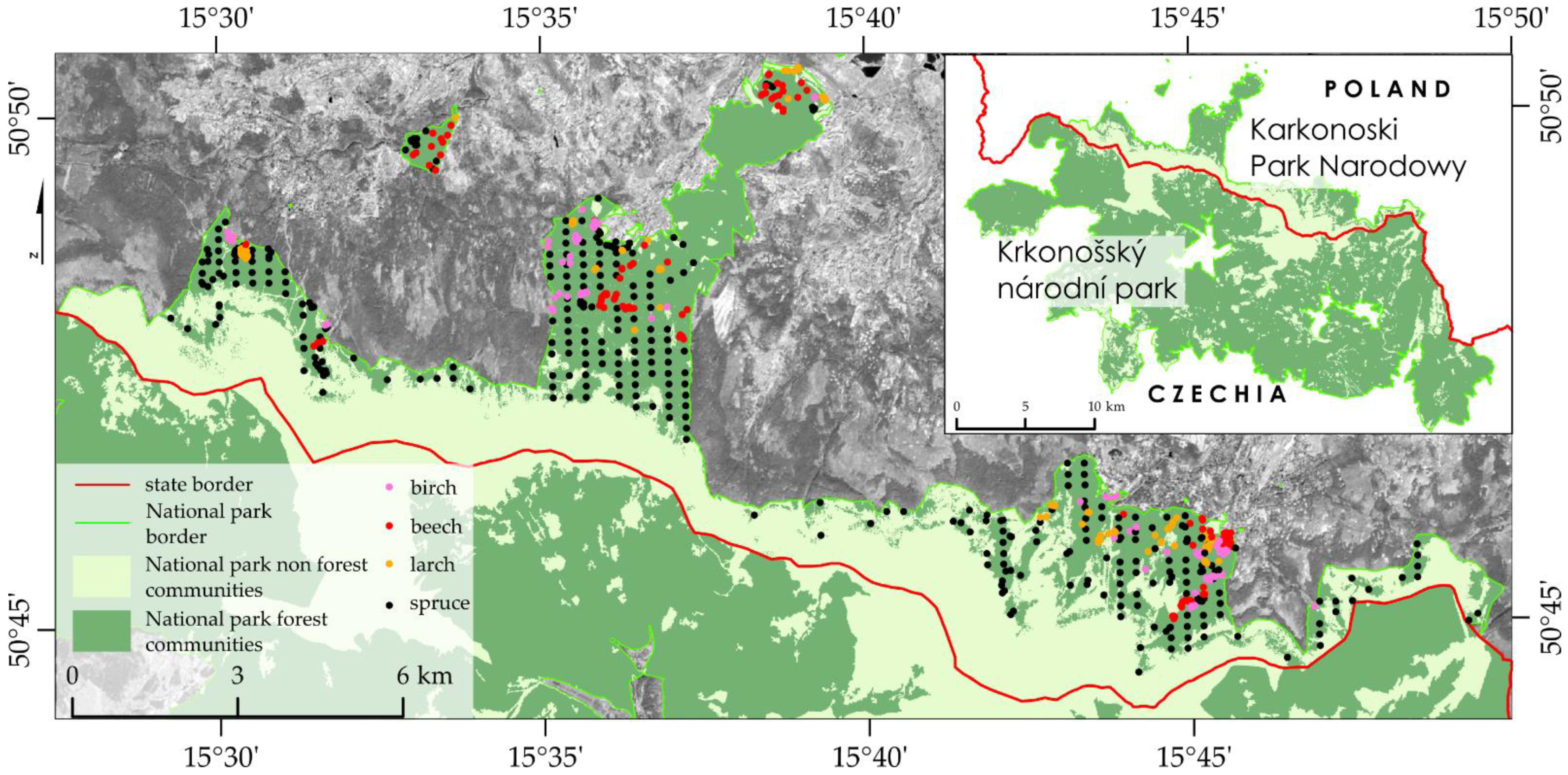
In our opinion, there is no alternative to satellite research, because traditional research methods are key elements of the monitoring, which bases on a network of transects on which regular field observations are made (Figure 4). This is a very subjective method, because visual observations are made by different employees, so burdened with a large dose of uncertainty. In addition, research patterns are limited to selected locations, not the entire area of parks. The second important limitation are data acquisition and processing costs of airborne campaigns, so an airborne research is relatively rare and performed in a time, which makes it difficult to capture phenological changes taking place. In case of our study, law regulations are an additional problem, because the Reserve is located under the board of legally and financially independent entities, complying with various national guidelines. Satellite images, especially Sentinel-2, are acquired every few days free of charge. High time resolution allows to create masks eliminating clouds and shadows, which is common in mountainous areas. Cloud free images with high acquisition frequency captures environmental changes. The key element is the fact that the size of the smallest pixel (10 m) coincides with the tree crowns, which allows for detailed analyzes.

To compare the obtained results with achievements of other researchers (references), we limited the discussion to papers in which authors used Sentinel-2 and Landsat imagery, machine learning algorithms additional data increasing classification results (e.g., vegetation indices, derivatives of terrain models), and identified the same species as us. (Table 6). Due to the pixel size, much of the work focused on classifying the dominant tree species or the forest types in which these species predominate. In this study, when Sentinel-2 imagery and the SVM-RBF algorithm were used, the following producer accuracies were achieved: spruce (93%), birch (85%), beech (83%), and larch (67%). In a study by Hościło and Lewandowska [80], in which forest stands of the Tatra Mountains were classified using Sentinel-2 imagery, the Digital Terrain Model (DTM), and the Random Forest classifier, the following producer accuracies were obtained: spruce (71%), larch (87%) birch (77%), and beech (91%). Significantly better results were obtained for spruce and birch, while poorer results were obtained for larch and beech. The differences in the results could be due to the different characteristics of the studied stands, the application of a different method that increased the information content of images, and the use of data from other sensing periods. A similar classification was performed by Persson et al. [81], who obtained the following producer accuracies using MSI data and the Random Forest: spruce (88%), larch (95%) and birch (81%). The classification of larch (95.5%) was much weaker than in the mentioned work, but the results for spruce (88.2%) and birch (80.8%) were quite comparable. The smaller number of test polygons includes 10% of the dataset; hence, the differences in the classification accuracies may have resulted from insufficient validation. Another example is the classification performed with Sentinel-2 data and the Random Forest classifier by Immitizer et al. [44], which achieved the following producer accuracies: spruce (85%), larch (44%), and beech (49%). Only spruce was classified at a similar level with our scores, other species achieved worse results, but comparing all the results with Hościło and Lewandowska [80] we can speculate that the reason is the compactness of the tree crowns, because in the Tatras these species form homogeneous patches, and thus the obtained results are the best one, in individual parts of the Karkonosze there are also small but compact habitats, hence the high classification results, but worse than in the Tatras. Classification using the Maximum Entropy algorithm and Landsat 8 data enhanced with DTM was carried out in a mountainous area by Chiang et al. [15] and produced producer accuracies of 77% for larch and 55% for birch. For both species, the results obtained in the current study were lower, and this discrepancy can be explained by the classifier used and the additional data. When analyzing the additional data used in the study to increase the informativeness of the image, the best accuracy levels are obtained by studies with multi-temporal compositions. Penna and Brenning [42] obtained the highest overall accuracy among comparable studies at 94% using NDVI and NDWI indices, a multi-temporal composition, and the Random Forest algorithm on OLI scanner data. A high value (88%) was also obtained by Persson et al. [81] using only a multi-temporal composition, the same algorithm for classification, and MSI scanner data. The overall accuracy (85%) obtained in the current study was slightly lower but not significantly different from that obtained in the above works. Due to relatively small terrain denivelations and low height differences between montane and foothills zones (mountains were formed during the Hercynian orogeny), we chose not to use DEM data and others topographic attributes, which does not always provide confidence in the classification accuracy, whereas both the Pimple et al. [43] and Li et al. [31] studies showed increases in the classification accuracy by only 1 to 3%. Despite the relatively low F1-scores for larch, the results are very valuable because larch does not cover naturally large homogeneous areas. It is often planted linearly to protect stands from strong winds, which cause significant damage due to windbreaks. Additionally, the nature of the Krkonoše forest stands means that most species, apart from spruce, are distributed at similar altitudes, which justifies the lack of use of DEM data in the study.

The overall accuracy (77–87%) results are quite comparable to those obtained by other authors. Better results may be achieved for forest ecosystems where individually studied species occur in more dense groups. It may also depend on the adopted number of validation polygons, i.e., whether there is a significant number of them (more than 50% of the data). Other authors have mostly used 30% of the data, or even 10%, as in Persson et al. [81], for verification, which may significantly distort the assessment of classification accuracy. In examples where there is no attachment of additional data to the image, lower overall classification accuracies are obtained, which confirms the need to make multispectral data more informative using a multitemporal composition. The MSI scanner has more channels and has a better spatial resolution than the OLI scanner, and significant differences in the classification quality were observed in favor of the MSI sensor. It achieved higher overall accuracy results (4–7%) for all classifiers except the Random Forest, where the OLI instrument provided better results (by 2%). A good example is the comparison of classifications made by Soleimannejad et al. [82], where the difference in overall accuracy between the MSI and OLI instruments was 1%. Puletti et al. [23] distinguished among three forest classes based on multitemporal compositions and the following vegetation indices: NDVI, the Plant Senescence Reflectance Index (PSRI) [83], the Red Edge Normalized Difference Vegetation Index (RENDVI) [84], and the Anthocyanin Reflectance Index (ARI) [85]. A total of 42 channels were obtained and these were classified by Random Forest. The producer accuracy ranged from 83% to 91%.

Table 6. Comparison of the obtained results with those reported in the literature.

Author	Tree Species (PA %)				OA (%)	Algorithm	Satellite	Number of Classes
	Birch	Beech	Larch	Spruce
[86]	27.2	98.0	74.7	53.3	90	RF	S-2	9
[80]	83.7	91.5	86.5	70.5	82	RF	S-2	8
[44]	-	48.8	44.0	85.3	63	RF	S-2	6
[81]	80.8	-	95.5	88.2	87	RF	S-2	5
[87]	-	-	88.1	75.8	87	RF	S-2	5
[88]	80.0	-	-	91.9	87	Bayesian inference	S-2	4
[15]	55.0	-	96.0	-	81	Maximum Entropy	L 8	4
[23]	-	95.5	-	88.2	86	RF	S-2	4
[12]	98.8	-	-	-	95	SVM-RBF	S-2	14
[89]	-	63.0	-	73.0	63	RF	S-2	6
[90]	97.7	-	-	-	97	RF	S-2	4
[36]	-	79.0	-	-	85	RF	S-2	5
[91]	-	-	-	74.2	79	RF	S-2	4
Our results	72.5	71.6	68.3	90.8	83	SVM RBF	L 8	4
	73.9	75.8	71.0	92.7	85	RF
	59.7	67.0	56.4	91.3	77	ANN
	84.8	82.7	67.0	92.6	87	SVM RBF	S-2
	74.5	81.0	71.0	89.8	83	RF
	72.9	82.4	62.6	93.8	84	ANN

Table 6. Comparison of the obtained results with those reported in the literature.

Author	Tree Species (PA %)				OA (%)	Algorithm	Satellite	Number of Classes
	Birch	Beech	Larch	Spruce
[86]	27.2	98.0	74.7	53.3	90	RF	S-2	9
[80]	83.7	91.5	86.5	70.5	82	RF	S-2	8
[44]	-	48.8	44.0	85.3	63	RF	S-2	6
[81]	80.8	-	95.5	88.2	87	RF	S-2	5
[87]	-	-	88.1	75.8	87	RF	S-2	5
[88]	80.0	-	-	91.9	87	Bayesian inference	S-2	4
[15]	55.0	-	96.0	-	81	Maximum Entropy	L 8	4
[23]	-	95.5	-	88.2	86	RF	S-2	4
[12]	98.8	-	-	-	95	SVM-RBF	S-2	14
[89]	-	63.0	-	73.0	63	RF	S-2	6
[90]	97.7	-	-	-	97	RF	S-2	4
[36]	-	79.0	-	-	85	RF	S-2	5
[91]	-	-	-	74.2	79	RF	S-2	4
Our results	72.5	71.6	68.3	90.8	83	SVM RBF	L 8	4
	73.9	75.8	71.0	92.7	85	RF
	59.7	67.0	56.4	91.3	77	ANN
	84.8	82.7	67.0	92.6	87	SVM RBF	S-2
	74.5	81.0	71.0	89.8	83	RF
	72.9	82.4	62.6	93.8	84	ANN

The process of classification and accuracy assessment requires an appropriate amount of up-to-date and reliable training and verification patterns. The optimal solution is field research allowing for detailed identification and determination of representative patterns, but the procedure is time consuming and expensive, especially in mountainous areas. So, the influence of the number of pixels on the classification accuracy was tested, allowing to determine the necessary number of training pixels to obtain satisfactory results. The highest results were achieved when there were 300 pixels, and this was considered the most optimal number of samples per class. Similar conclusions were reached by Sabat-Tomala et al. [92] who also tested the Random Forest and Support Vector Machine classifiers using the same threshold values on plant species. Nevertheless, the use of 100–150 pixels/class in the training patterns resulted only 2–3 percentage points lowered the results (Figure 7). It has a practical dimension allowing to shorten field research, without a significant loss of obtained results. In general, in research works where the effects of classifier choice, reference sample size, and reference class distribution on classification accuracy per pixel have been tested, various conclusions have been obtained [93,94]. Noi and Kappas [93] concluded that the performance of the RF classifier on different Sentinel-2 satellite image data with different training sampling strategies (balanced or unbalanced) differs. They observed that the training sample sizes for land cover classes were large (greater than or equal to 500 pixels/class), and the performance of the kNN, RF, and SVM on balanced and unbalanced datasets did not differ significantly.

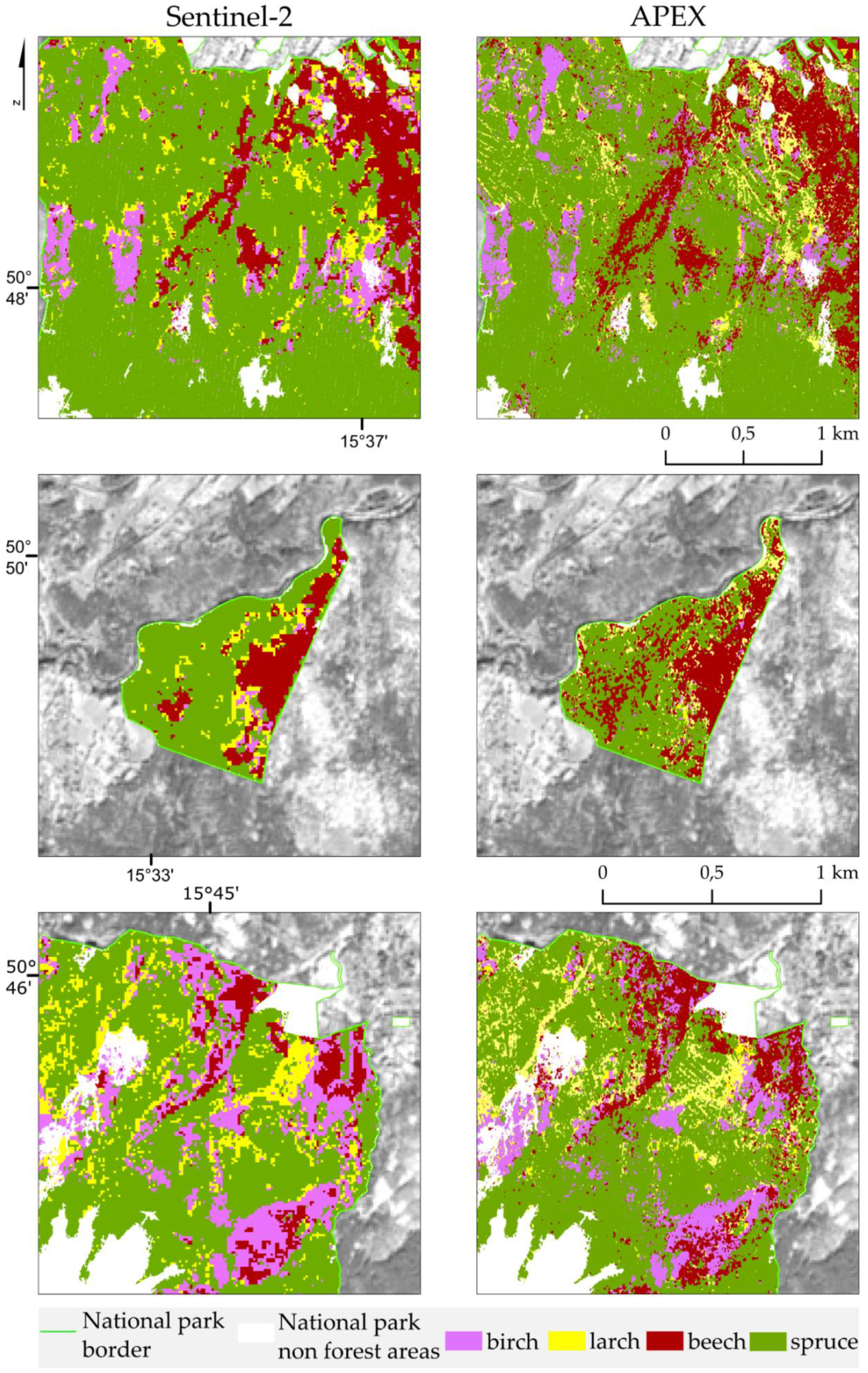
Comparing the airborne APEX hyperspectral (9 m² pixel size, 288 spectral bands), multitemporal Sentinel-2 (100 m², 12 bands) and Landsat 8 (900 m², 10 bands) images, the best classified species was spruce (around 90% in case of all classifiers), which dominates in the parks. However, the large area covered led to relatively homogeneous images being produced for satellite and APEX airborne images (Figure 10). The worst results were obtained for larch in both Landsat and Sentinel-2 images (71% based on Random Forest). These seemingly worse results, however, are very satisfying, because larch does not cover dense polygons but is often planted in the form of linear transects. Despite spectral and spatial differences of the images, visual interpretation of the APEX and the Sentinel-2 based maps confirms the usefulness of the satellite images for identification of woody species (Figure 10). In each of the presented study areas, the localization of particular species on Sentinel-2 images is proper; however, difficulties arise for deciduous species (birch and beech) on sites where they overlap, as there is a tendency to overestimate and underestimate classes. When a species forms a compact stand, its identification is much more accurate than in the case of communities consisting of small groups of trees. Due to the fact that spruce is the dominant community, there were no difficulties in mapping it. The biggest challenge occurred with the larch, which rarely grows in dense groups, because it is most often planted in strips as protection from strong winds for other growing trees. It should be considered that maps prepared on the basis of Sentinel-2 data are valuable and satisfactory, as they can show the characteristics of tree stands, allowing quick, straightforward, and cheap analyses and being especially useful in mountain areas with limited accessibility to many tree communities.

In this study, four classes were used for classification; this number is similar to that used in other studies, but as mentioned before, due to the nature of the stand and spatial resolution, it was not possible to identify other species. There have been cases where more classes were designated, with seven [44] or eight [80] species distinguished. However, the number of species distinguished depends on the tree stand species structure and the proportion of individual species. The results obtained can be considered highly accurate and relevant due to the fact that the reference sites are distributed regularly over the park, giving results that are closer to reality. Despite using more data in the main classification, the study shows that it is possible to achieve a fairly good overall classification accuracy (87%) by combining three images from spring, summer, and autumn. However, it should be noted that the studied stands are located in a mountainous area, where the development of vegetation starts late, so better results could be obtained with a scene from later in spring, but such analyses were prevented by the cloud cover over the Park area [95].

Comparing the classifiers used, it can be concluded that the Random Forest is the most commonly used by researchers to obtain satisfactory results, and the SVM has a comparable level of usage [12,16]. A meta-analysis comparing peer-reviewed studies on RF and SVM classifiers was conducted by Sheykhmousa et al. [96]. For low spatial resolution images, the RF method consistently provides better results than the SVM, but a comparison of the average accuracies of the RF and SVM methods suggests the superiority of the SVM method when classifying data containing significantly more features. It is much less common to use other classifiers, such as, Maximum Entropy, which was used in the study by Chiang et al. [15], or deep neural nets, which are used in very complex image structures, e.g., to identify individual tree species in cities. In large and homogeneous forest areas, the classifier architecture optimization is a time-consuming procedure, and the obtained results do not compensate for the workload associated with the preparation of the classifier [97,98]. Due to the prevalence of studies that use the Random Forest algorithm and the high classification accuracy results it achieves, it can be considered one of the most suitable algorithms for this kind of research. However, in our opinion, it is also necessary to test other classifiers, as our study showed higher accuracy results for SVM.

5. Conclusions

In this paper, the usefulness of Sentinel-2 and Landsat 8 images was verified by applying the RF and SVM algorithms to identify forest species. An essential element of the work was the research area (biosphere reserve), where forest stands are characterized by growing on heterogeneous sites with highly variable species of different ages (physical parameters) and with co-occurring objects (dead trees, rocky surfaces, trails). Thus, proper classification was significantly more difficult than in managed forests, because it took place in a highly protected area where traditional forest management is not allowed. The obtained overall accuracy and producer accuracy values are comparable to those obtained in similar studies conducted by other authors on standard commercial forests, where dying trees are successively eliminated and monocultures are preferred due to the ease of treatment. Outcomes confirmed that the species investigated have sufficiently specific spectral features that allow them to be recognized, and the application of nonparametric classifiers and their optimization procedures eliminated noise generated by co-occurring objects.

Classifications carried out with all algorithms, both in the Landsat and Sentinel-2 images, confirmed good possibilities of identifying the spruce (over 90%), it is important in the time of climate change, because the spruce’s roots are located relatively shallow under the soil surface, being exposed to overdrying, leading to water stress for the tree, and thus at risk of being attacked by insects. Therefore, monitoring of the occurrence and water stress of spruce allows for the assessment of climate change. Other woody species were classified with good overall accuracies (Sentinel-2 images and the SVM RBF classifier offered an overall accuracy of 87%, Landsat 8 and RF achieved 85%, and ANN–84%), confirming their suitability for large-scale monitoring of the stand species composition.

Low-resolution multispectral data can only be used as a source of coarse data on the forest composition. Detailed information on forest cover can be obtained more reliably using airborne hyperspectral or multispectral imaging. Future studies using high-resolution orthophoto maps and advanced ML techniques for tree species identification are required.

While the use of remote sensing data cuts the costs of operation when compared with standard forest management methods, it relies heavily on having accurate and up-to-date reference data. Moreover, the conducted classifications have confirmed that the size of the training patterns can be reduced to 100–150 pixels/class, and the obtained results are only two-four percent points worse comparing to maps based on 300 pixel sets. This is valuable information, because the field verification of mountain areas, and especially protected areas, is very difficult as exploring the area is challenging (no roads, denivelations and large research area).

Originally the 60 m pixel size B1 and B9 bands, which are used as standard for atmospheric correction, showed 10–11% of MDA, which is only 50% less comparing to the most informative B6, NDVI, or B4, and their informativeness is comparable to other bands, e.g., B7, B8, so, the bands should not be omitted.

The proposed research methodology allowed to obtain results comparable to classifications of economically used forest areas, where dominate homogeneous forest stands in terms of species and age prevail. This means that both satellite images contain sufficient spectral features, and tree crown sizes have of appropriate size in relation to the pixel size, which allows for proper classification based on non-parametric classifiers. The measurable and documented result of the work is a map of the entire area of two neighboring countries, which is a valuable comparative material for traditional forest research.