A New Model of Quasigeoid for the Baltic Sea Area

Abstract

The Space Research Centre in Warsaw is participating in the ESA project “Geodetic SAR for Height System Unification and Sea Level Research”. To observe the absolute sea level and enable the unification of the height systems, the physical heights of the tide gauge stations referring to a common equipotential surface (quasigeoid/geoid) are needed. This paper describes the new quasigeoid model for the area of the Baltic sea. The quasigeoid calculation was carried out according to the Helmert method, in which the topography is condensed on a layer lying on the geoid. Airborne gravity anomalies from the Baltic area and terrestrial anomalies from Sweden, Finland, Denmark, Lithuania, Latvia, and Poland were used. The necessary terrain corrections have been computed from a digital terrain model based on the SRTM30 model. To compute the long-wavelength part of the quasigeoid, the geopotential models GOCE-DIR6, GOCO06s, and EIGEN-6C4 were used; therefore, the three solutions have been obtained. All calculations were done in a zero-tide system. The new quasigeoid model is obtained on a regular 1.5’ × 3.0’ grid in the GRS80 reference system, covering the Baltic Sea and the surrounding area 52° < ϕ < 68° and 11° < λ < 30°. These gravimetric quasigeoids were compared to quasigeoid undulations derived at 29 GNSS/leveling points of the ASG-EUPOS permanent network, located in the study area. Our calculations show that the accuracy of the calculated quasigeoids is almost the same in all three cases and is about ±0.04 meters. Finally, quasigeoid anomalies were interpolated at the Polish tide gauge stations. The new gravimetric quasigeoid solution could be very important for height system unification, for geophysical purposes as well as for engineering purposes.

1. Introduction

The Space Research Centre in Warsaw is participating in the ESA project “Geodetic SAR for Height System Unification and Sea Level Research”. To observe the absolute sea level and enable the unification of the height systems, the physical heights of the tide gauge stations, referring to a common equipotential surface, e.g., the geoid, are needed [1].

The geoid is of fundamental importance for geodesy, oceanography, and physics of the solid Earth and was introduced by C.F. Gauss as a refined model of the figure of the Earth [2]. In geodesy, the geoid/quasigeoid is a reference surface for vertical datum [3], orthometric heights [4], a transformation of ellipsoidal heights into orthometric heights [5], local and regional vertical datum unification [6], and satellite orbits prediction [7].

The first gravimetric geoid for Scandinavia and the part of Poland was computed in 1949 [8]. Due to the small amount of gravimetric data that was achievable at the time, the accuracy of this geoid model was very low.

Due to political changes in Eastern Europe in the 1980s, gravimetric data were released and used to compute the first fairly accurate quasigeoid in Poland. The quasigeoid for the Polish part of the Baltic region was computed in 2006 by W. Jarmołowski [9]. The last Polish quasigeoid for the Baltic Sea was computed in 2019 [10]. Several geoid/quasigeoid computations for the Baltic countries and Baltic Sea were performed in the last 20 years, e.g., [11,12,13] and others.

These consecutive geoid models have been progressively improved over the years by implementing a better theory, conducting gravity surveys to fill large data void areas, compiling more precise Digital Terrain Models (DTM) [14], and embedding more accurate global gravity models derived from dedicated GOCE (gravity field and steady-state ocean circulation explorer) and GRACE (gravity recovery and climate experiment) satellite gravity missions [15].

The paper aims to calculate an accurate quasigeoid for the Baltic area. The purpose of this work is to calculate the quasigeoid model in the Baltic sea area to explore the possibilities of SAR technology for Baltic height system unification and Baltic sea level research.

2. Materials and Methods

In the classical approximation, the geoidal undulation can be estimated by Stokes’ formula

$$N=\frac{R}{4\pi \gamma }{{\displaystyle \iint }}_{\sigma }^{}\mathsf{\Delta }gS\left(\psi \right)d\sigma$$

(1)

where R is the Earth’s radius, Δg is the gravity anomaly, γ; is normal gravity, and S(ψ) is Stokes’ function, provided the topography has in some way been removed or shifted inside the geoid.

Gravity is usually measured on the Earth’s surface. To calculate the geoid using Stokes’ formula, the gravity (or gravity anomaly) must refer to the geoid and not to the Earth’s surface. The gravity must be reduced to the geoid. This may be done using one of several available methods. In [16], reduction methods such as the Bouguer, isostatic, Rudzki, and Helmert methods are mentioned. Additionally, the gravity may be reduced by the residual terrain model (RTM) method [17].

Thus, the gravity anomaly in Equation (1) has to be reduced to the geoid by applying free-air reduction, assuming there are no topographic masses

$$\mathsf{\Delta }g=g+\delta g_F-{\gamma }_0$$

(2)

These masses are then placed on the surface of the geoid in the form of a layer with a density $\kappa =\rho \times \mathsf{H}$. This method of placing topographic masses on a geoid is called the Helmert condensation method.

The displacement of the topographic masses changes the gravitational field of the Earth, including the potential of the geoid (Figure 1). The level surface that possesses the geoid potential after displacement is called the cogeoid: therefore, the equipotential surface computed from Stoke’s integral is the cogeoid instead of the geoid. The vertical distance between the geoid and the cogeoid N_ind can be computed according to [18] from

$$N_{ind}\approx -\frac{\pi G\rho }{{\gamma }_m}{H}_P^2$$

(3)

which converts the cogeoid into a geoid.

To compute the cogeoid, additional reduction of the gravity value from the geoid to cogeoid is necessary (secondary indirect effect) and here, the free-air reduction is sufficient

$$\mathsf{\Delta }{g}_{ind}\approx \frac{2\pi G\rho }{R}{H}^2$$

(4)

This term is usually much smaller than 1 mGal and is often neglected.

To obtain the quasigeoid the geoid undulation, N minus height anomaly ζ is needed. This separation is given in [16] as

$$N-\zeta \approx =\frac{\Delta g_B}{{\gamma }_m}H$$

(5)

where Δg_B is the Bouguer anomaly, and γ_m is the mean normal gravity (9.81 ms⁻²).

To get the true value of the geoidal undulation, the integration should be extended to the whole sphere. For local or regional geoid computation, usually, a global geopotential model (GM) is combined with discrete local gravity data as well as height data. The geopotential model provides the low-frequency or long-wavelength part of the geoid. Local gravity anomaly data and height data provide the medium- and high-frequency components of the geoid spectrum, respectively [19]. The formula for the practical computation of the local geoid by the remove–restore technique is

$$N=N_{GM}+N_{\mathsf{\Delta }{g}_{res}}+N_{ind}$$

(6)

where N_GM is the geoidal undulation implied by the geopotential model, $N_{\mathsf{\Delta }{g}_{res}}$ is the contribution of the terrain-corrected mean free-air gravity anomalies reduced to the reference field, and N_ind is the indirect effect of the terrain reduction.

The contribution of the GM coefficients can be computed by the spherical harmonic expansion formulas [2] given below

$$N_{GM}=N_0+\frac{GM}{r{\gamma }_0}{\displaystyle \sum }_{n=2}^{n_{max}}{\left(\frac{a}{r}\right)}^n{\displaystyle \sum }_{m=0}^n\left(C_{nm}cosm\lambda +S_{nm}sinm\lambda \right)P_{nm}\left(sin\phi \right)$$

(7)

where G is the gravitational constant, M is the mass of the Earth, r is a geocentric radius, a is semimajor of the reference ellipsoid, C_nm and S_nm are the fully normalized harmonic coefficients of the anomalous potential, and P_nm is the fully normalized associated Legendre functions, γ₀ is the normal gravity on the ellipsoid, and N₀ results from the difference in the mass of the Earth used in the IERS Convention and GRS80 ellipsoid.

The geoid or quasigeoid is estimated using Stokes’/Molodensky’s formulae with gravity anomalies, Δg, as input data. Before applying Stokes’ formula, the gravity anomaly must be reduced by the removing–restoring technique (R – R) [20].

$$\mathsf{\Delta }{g}_{res}=\Delta g_{FA}+\mathrm{c}+\mathsf{\delta }\mathsf{\Delta }\mathrm{g}-\mathsf{\Delta }{g}_{GM}$$

(8)

where the first term on the right-hand side of Equation (8) is the mean free-air gravity anomaly corrected for atmospheric attraction, the second term c is the classical terrain correction, given in linear approximation by [21]. The third term in Equation (8) is the indirect effect on gravity, which, being very small (usually much smaller than 1 mGal), was neglected, and the fourth term is the reference anomaly computed by Equation (7)

$$\Delta g_{GM}=\frac{GM}{r^2}{\displaystyle \sum }_{n=2}^{n_{max}}\left(n-1\right) {\left(\frac{a}{r}\right)}^n{\displaystyle \sum }_{m=0}^n\left(C_{nm}cosm\lambda +S_{nm}sinm\lambda \right)P_{nm}\left(sin\phi \right)$$

(9)

In principle, the residual part of the geoid undulation $N_{\Delta g_{res}}$ can be obtained by evaluation of the Stokes integral by discrete summation [16]. The summation has to be repeated for every point.

For the computation of large-scale regional geoids, the summation has to be repeated for every point. For the computation of large-scale regional geoids, such as the current Baltic geoid with a 640 × 380 grid, the computational task is too big to be handled efficiently, even on medium-sized or large computers, not to mention microcomputers.

Therefore, the FFT-based numerical methods, which allow for a fast evaluation of discrete convolutions using all the data on the grid, are the only methods that allow for a fast evaluation of discrete convolutions using all the data on the grid and are the only realistic approach to the problem. Currently, several FFT-based techniques are available for the evaluation of the discrete Stokes integral. Two of those, namely the 2D spherical FFT and the multi-band spherical FFT [22] methods, are in use.

Zero Degree

As long as IAG does not release a new geodetic reference system, GRS80 should be used for the regional geoid/quasigeoid computation, i.e., for the computation of gravity anomalies, disturbing potential, ellipsoidal coordinates, geoid heights, height anomalies, etc. A zero-degree correction has then to be added to reach the latest GM value and the conventional reference value W₀. The zero-degree term for the geoid separation is given by [2]

$$N_o=\frac{GM-G{M}_o}{R\gamma }-\frac{W_o-U_o}{\gamma }$$

(10)

where the parameters GM_o and U_o correspond to the normal gravity field on the surface of the normal ellipsoid. For the GRS80 ellipsoid, we have GM_o = 398,600.5 × 10⁹ m³s⁻² and U_o= 62,636,860.85 m²s⁻² [2]. The Earth’s parameters GM = 398,600.4415 × 10⁹ m³s⁻² (IERS Conv. 2010) and W_o = 62,636,858.18 m²s⁻² [1] were used in quasigeoid/geoid computation from geopotential. The mean Earth radius R and the mean normal gravity γ on the reference ellipsoid are taken to be equal to 6,371,008,771 m and 9.798326 m s⁻², respectively (GRS80 values). Based on the above conventional choices, the zero degree term from Equation (10) yields the value N_o = −0.665 m, which has been added to the geoid heights obtained from the spherical harmonic coefficients series expansions of all geopotential models.

3. Data

3.1. Gravity Data

Our calculations use gravimetric data from various sources, and these data are described below.

Mean Faye’s anomalies in 1’ × 1’ blocks for Poland’s territory are from the Institute of Geodesy and Cartography in Warsaw. These data have been calculated from gravimetric point data carried out in the years 1957–1979, from the detailed survey and gravimetric profiles referred to as the Potsdam gravity system. Horizontal coordinates were expressed in the national ”Borowa Góra” geodetic reference system. All gravimetric measurements have been linked to the national leveling network (Kronstadt60) with an accuracy of +5 cm. Gravimetric measurement accuracy is estimated as ± 0.11 mGal [23]. Then, all data were subsequently corrected to the IGSN71 network, transformed to the ETRS89 reference system [24], and corrected for the terrain corrections and atmospheric correction. Then, mean Faye’s anomalies were calculated in 1’ × 1’ blocks using elevation data from the gravimetric database and the DTED2 model by collocation method [25]. Gravity anomalies are in the mean-tide system [26].

Mean free-air anomalies in 1’ × 1’ blocks for the Baltic south area are from the Space Research Centre PAS. These anomalies were calculated from a gravimetric survey taken between 1978 and 1980 by the teams of the Moscow Research Institute. Measurements were made along the profiles using gravimeters of Soviet construction. The point position error in the horizontal plane was estimated ±80 m. The depth of the sea was determined by sonar with an accuracy ± of 1.4 m. After taking into account the necessary corrections, the error of determining free-air anomalies was estimated as ±0.57 mGal. The geographical coordinates are determined in the “Borowa Góra” horizontal reference frame and the heights in the Kronstadt60 vertical system. Finally, anomalies were calculated based on the formula for the GRS80 normal field and referred to as IGSN71. These data do not contain atmospheric corrections. Mean free-air anomalies in a 1’ × 1’ grid were calculated with the collocation method [27]. Computed gravity anomalies are in the mean-tidal system.

Mean 5’ × 5’ free-air gravity anomalies from Finland were provided by the Finish Geodetic Institute. Anomalies in 5’ by 5’ blocks were generated from the Finnish gravity register. The anomalies are free-air anomalies computed using the gravity formula of the GRS80 system. No terrain corrections were applied. The coordinates referred to grid cell center points, while the grid cell edges are on “even” latitudes/longitudes (“Forsberg convention”). The heights used are in the Finnish height system NN60. Horizontal coordinates are in the Finnish Map Grid Coordinate System (KKJ), which differ by several hundred meters from both ED50 and ED87 coordinates. The accuracy of anomalies computed in such a way is estimated to fluctuate within ±2 mGal [28]. Gravity anomalies are in the tide-free system [29].

Airborne gravity data were from Kort and Matrikelstyrelsen in Denmark. A set of point aerial gravimetric profiles, from the project on the Baltic Sea, was carried out in 1999. The measurements were performed with the use of a high-class gravimeter stabilized on a vibration-damping platform. Data from airborne gravimetric measurements (free-air anomalies) are linked to gravimetric points in the IGSN71 system at airports. The position is determined by GNSS observation related to numerous reference stations linked to the ITRF94. Consistent r.m.s. error estimates for r surveys range from ±1.5 to ±2 mGal [30]. Gravity anomalies are in the zero-tide tidal system [29].

Shipborne gravity and land data were from Kort and Matrikelstyrelsen in Denmark. In 1994 and 2004, point data from the land and sea area of Denmark, point data from the Eastern part of Germany, point sea measurements and mean anomalies from gravimetric maps from the Kaliningrad area, and point data from Lithuania and Latvia were obtained during our training at the KMS in Denmark. Gravity data are in the GRS80 system and are referred to as IGSN71 [9].

Gravity data from Sweden were obtained from the Bureau Gravimétrique International and include g value as well as free-air anomalies and some other useful information. Data are expressed in the GRS80 system and IGSN71. Atmospheric corrections have been made to this data. Gravity anomalies are in the zero-tide tidal system [29].

Gravimetric data were obtained from GETECH, a West–East European gravity project (WEEGP) commenced in April 1991 and follows the completion of all available land and marine gravity data for the area 35° < ϕ < 84° and 25° < λ < 60°. The database was used to generate an 8 × 8 km grid of interpolated free-air and Bouguer values for the region. All gravity data have been reprocessed using the IGSN71 gravity datum and GRS80 gravity formula. A Bouguer density of 2.67 g/cm² was used. Terrain and Earth curvature corrections have been applied to the Bouguer gravity data. Terrain corrections were calculated to a distance of 166.7 km for each gravity station [31]. In 2004, ZGP CBK PAN obtained gravimetric data from GETECH for the area of 14° < ϕ < 30°, 44° < λ < 60°. In our calculations, GETECH data were used only for parts of Ukraine and Belarus. Probably, gravity anomalies are in the mean-tidal system.

Gravity data were from the EGM2008 model [32], and additionally for the data gaps in the Gulf of Riga, the free-air gravity anomalies in a grid 2’ × 2’ were computed from the geopotential model EGM2008.

All gravimetric data referred to the normal gravity defined by the GRS80 system and referenced the IGSN71 gravity network. Moreover, where necessary, atmospheric and terrain corrections were added.

Gravity data were from Poland, the southern Baltic region, and GETECH data were converted from a mean-tidal system to a zero-tide system according to the formula [33]

$$g_z=g_m+30.4-91.2si{n}^2\phi \mathsf{\mu }\mathrm{Gal}$$

(11)

Gravity data from Finland have been converted from a tide system to a zero-tide system according to the formula [33].

$$g_z=g_n+\left(\delta -1\right)\left(-30.4+91.2si{n}^2\phi \right) \mathsf{\mu }\mathrm{Gal}$$

(12)

Combined Data Set

To calculate the geoid/quasigeoid in the Baltic region from the above-mentioned data, a joint gravimetric data set was created, which is shown in Figure 2 (statistics in

Table 1. Statistics of the gravity data used in this study (in mGal).

Data	n	Mean	Std dev	Min	Max
Combined data set	150,842	−7.0	16.7	−102.6	212.5

).

3.2. DTM Data

Any gravimetric geoid computation based on the Stokes’s integral must use anomalies that have been reduced to the geoid, usually using Helmert’s second method of condensation [16]. This involves the computation of the terrain correction and the indirect effect on the geoid, which are computed from a DTM. In the present study, a gridded topography 1.5’ × 3.0’ from SRTM 30 was used in Figure 3.

SRTM30, the new global topography, is a substantial improvement on the widely used global bathymetry [34]. Land and ice topography comes from the SRTM30 [35] and ICESat topography [36], respectively. Ocean bathymetry is based on a new satellite–gravity model where the gravity-to-topography ratio is calibrated using 298 million edited soundings.

3.3. Global Geopotential Models

A global geopotential model is necessary to calculate N_GM Equation (6) and Δg_GM Equation (8) in geoid/quasigeoid modeling. The first global model describing the gravity field was developed by Żongołowicz in 1956. Since then, significant progress has been made in computing global geopotential models.

Initially, geopotential models were counted from observations of satellite perturbations, followed by the combined development of satellite perturbations and terrestrial and ocean gravity anomalies. The land anomalies are contaminated by systematic errors due to various regional vertical reference systems [37]. Since biased heights enter into the computation of terrestrial gravity anomalies, which in turn are used for geoid determination, the biases enter as a secondary or indirect effect also in such a geoid model. In contrast to terrestrial gravity anomalies, gravity and geoid models derived from satellite gravity missions, and in particular from GRACE and GOCE, do not suffer from those inconsistencies. Those models can be regarded as unbiased [38].

In this work, three geopotential satellite models were used, namely GOCO06s order and degree 300 [39], GOCE-DIR6 order and degree 300 [40], and combination model EIGEN-6C4 order and degree 2190 [41].

GOCO06s (2019) is the latest satellite-only global gravity field model computed by the GOCO (Gravity Observation Combination) project. It is based on over a billion observations acquired over 15 years from 19 satellites with different complementary observation principles. This combination of different measurement techniques is key in providing consistently high accuracy and the best possible [42] spatial resolution of the Earth’s gravity field

GOCE-DIR6 (2019) is a result of the gravity field. and steady-state Ocean Circulation Explorer (GOCE) gravity gradient data of the entire science mission and data from LAGEOS 1/2 and Gravity Recovery and Climate Experiment (GRACE) were combined in the construction of a satellite-only gravity field model to a maximum degree of 300. When compared to Earth Gravitational Model 2008, it is more accurate at low to medium resolution, thanks to GOCE and GRACE data. When compared to earlier releases of European Space Agency GOCE models, it is more accurate at high degrees owing to the larger amount of data ingested, which was moreover taken at a lower altitude.

EIGEN-6C4 (2014) is a static global combined gravity field model up to degree and order 2190. It has been elaborated jointly by GFZ Potsdam and GRGS Toulouse. The combination of the different satellite and surface data sets has been done by a band-limited combination of normal equations (to max degree 370), which are generated from observation equations for the spherical harmonic coefficients. A brief description of the applied techniques for the generation of such a combined gravity field model is given in [43]. The resulting solution to degree/order 370 has been extended to degree/order 2190 by a block diagonal solution using the DTU10 global gravity anomaly data grid.

3.4. GNSS and Leveling Data

To assess the accuracy of the calculated quasigeoid model, it is necessary to compare quasigeoid anomalies from GNSS observations and leveling ζ^GNSS/lev with height anomalies calculated from anomalies ζ^grav from gravity data on the points of the permanent ASG-EUPOS network.

The ASG-EUPOS permanent network was established in June 2008. The ASG-EUPOS is a multifunctional system for precise satellite positioning [44]. This network covers the entire Polish territory and consists of a total of 393 GNSS/leveling points, shown in Figure 4. The results of the observation, i.e., the ellipsoidal coordinates ϕ, λ, and h of the reference stations in the PL-ERTF2000 system are given on the web page ASG-EUPOS website and they are probably in the tide-free system.

All ASG-EUPOS stations are connected to the vertical reference system Kronstadt86. The Kronstadt86 system is the result of the measurement and adjustment of the leveling network measured from 1974 to 1982 [45]. The final adjustment of the entire network is the tide gauge in Kronstadt and was accepted in 1985. The standard deviation of adjusted height difference is equal ±0.844mm $\sqrt{L_{km}}$, where L_km is the length of the leveling line and the standard deviation of adjusted heights is between 6.5 and 11 mm [45]. Heights in the Krostadt86 reference system are tide-free heights.

4. Quasigeoid Computation

4.1. N and Δg from Geopotential Models

For geoid modeling, the gravity data were merged and analyzed, and all necessary reductions were introduced. We introduced atmospheric corrections and terrain corrections and converted all gravity data to a zero-tide system. Calculations of the geoid and quasigeoid models were carried out for the area 52° < ϕ < 68° and 11° < λ < 3.0° in a 1.5’ × 3.0’ grid using the GRAVSOFT software (Figure 5) [46].

In the first step, the geoid undulation N_GM and gravity anomalies ∆g_GM from the GOCO06s, GOCE-DIR6, and EIGEN-6C4 models were calculated for the area 52° < ϕ < 68° and 14° < λ < 30° with a grid of 1.5’ × 3.0’ using the application given on the ICGEG web page http://icgem.gfz-potsdam.de/home, accessed on 26 May 2021 [22]. Then, the residual anomalies were computed with Δg_GM calculated from the GOCO06s, GOCE-DIR6, and EIGEN-6C4 models, and residual anomalies were calculated according to the Formula (8).

4.2. Gravity Data Gridding

Since the gravity data set consists of point data distributed randomly, an interpolation process has to be applied to obtain a regular data grid.

The interpolation of residual gravity anomalies (

Table 2. Statistics of residual gravimetric anomalies (in mGal) calculated from different geopotential models.

Model	Mean	Std dev.	Min	Max
GOCO06s	−0.3	9.6	−114.2	182.8
GOCE-DIR6	−0.4	9.2	−117.1	186.4
EIGEN-6C4	−0.4	2.5	−141.2	174.7

) in a grid of 1.5’ × 3.0’ was made by a collocation method using a geogrid program. The method is based on an expansion of the spherical FFT method [47]. No modification of Wong–Gore Stokes function was used. The program applies for point interpolation of either weighted means or least-squares collocation (Kriging) using a second-order Markov covariance model, which was used in our study.

For this purpose, the necessary empirical functions of covariance were calculated using the empcov program, and the results of the calculations are given in Figure 6 and

Table 3. Parameters of the covariance functions of successive residual sets of gravity anomalies calculated from different geopotential models.

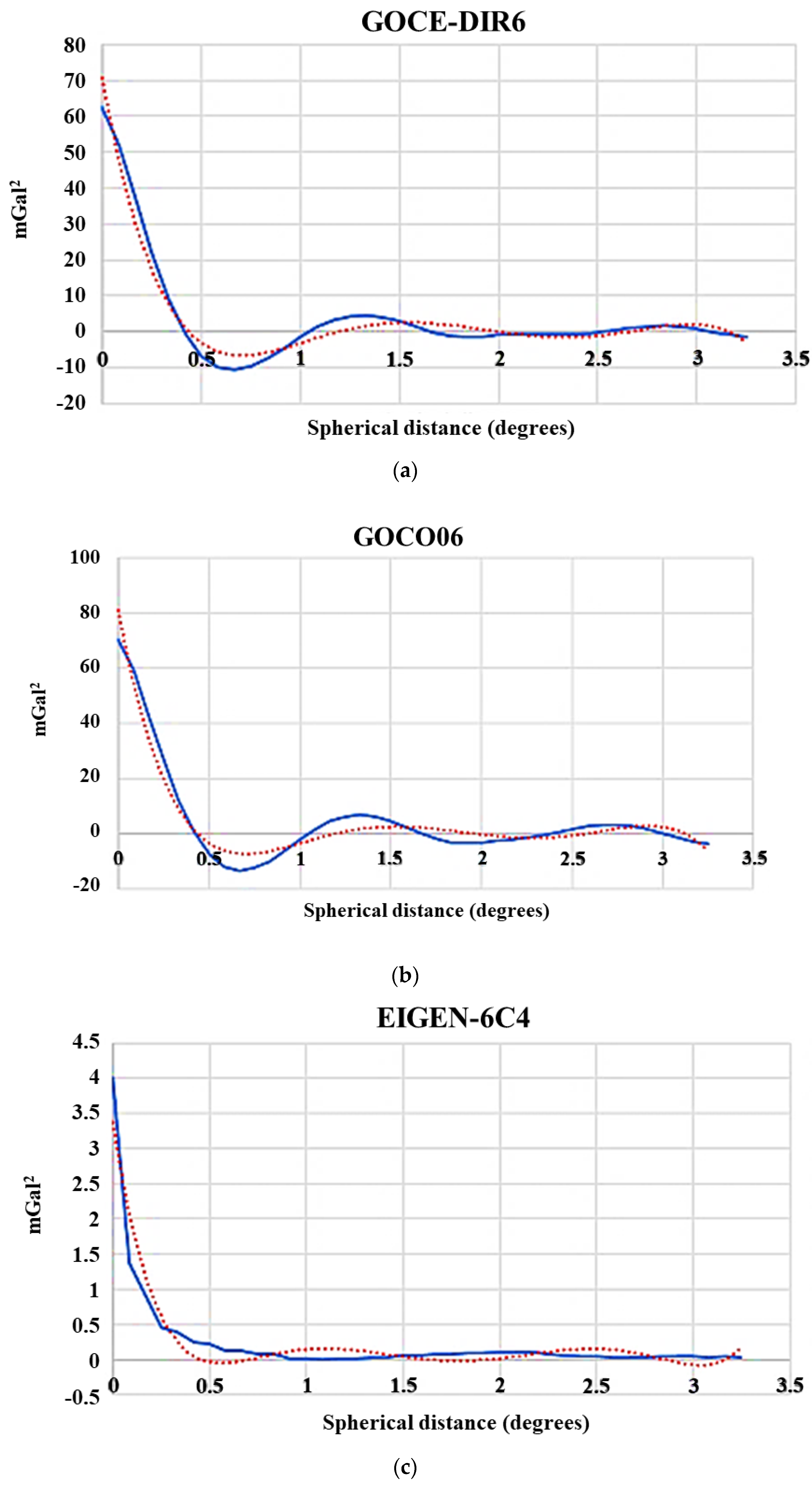
Model	Co mGal2	x km
GOCO06s	70.4	18.2
GOCE-DIR6	62.6	18.0
EIGEN-6C4	4.0	9.4

.

This enabled the calculation of residual anomalies in grid nodes 1.5’ × 3.0’.

4.3. Calculation of Residual Geoid

Having properly prepared gravity data, the calculation of $N_{\Delta g_{rez}}$ Equation (6) was conducted with the spfour program. The method used in the program is based on an expansion of the spherical FFT method [48]. The program uses analytical transforms of the FFT kernel; this allows additional control over the effective integration radius. No spherical harmonic Wong–Gore modification of Stokes’ integral was used in our computations (Figure 7).

The residual ellipsoid geoid separations were calculated for three different geopotential models and then the terms N_GM calculated in Section 4.1 were added, thus obtaining three cogeoids.

The next step was to calculate the term N_H from the Formula (4) and the quasigeoid corrections from the Formula (5). The following values were adopted in these formulae: G = 6.673 10⁻¹¹ m³kg⁻¹s⁻², ρ = 2700 kg m⁻³, and γ_m = 9.798 m s⁻². To calculate the corrections, a terrain model is required. In our case, we used the SRTM 30 model from Section 3.2. The calculated indirect effect and corrections to the geoid are shown in Figure 8. The indirect effect is from 0.00 to −0.17 m while the geoid corrections are −0.5 to 0.32 m. Adding to the cogeoid indirect effect and then the quasigeoid correction, we received three versions of quasigeoid models. The final quasigeoid map of the Baltic sea for the GOCO model is shown in Figure 9.

4.4. Qusigeoid Validation

To estimate the absolute accuracy of the gravity model the difference

$${\delta }_i=\left(h_i-H_i\right)-{\zeta }_i^{grav}$$

(13)

was computed in each point of the satellite GNSS network, where ${\zeta }_i^{grav}$ is quasigeoid from gravity data, and the mean value from

$$\widehat{x}=\frac{1}{n}{\displaystyle \sum }_{i=1}^n{\delta }_i$$

(14)

The empirical standard deviation is computed from

$$\widehat{\sigma }=\pm \sqrt{\frac{{{\displaystyle \sum }}^{ }{v}_i^2}{n-1}}$$

(15)

which gives the numerical description of the accuracy of the tested quasigeoid model (

Table 4. Assessment of the accuracy, in meters, of the subsequent quasigeoid models at the points of the ASG-EUPOS network and Kronstadt86 vertical system.

Model	Mean	Std dev	Min	Max
GOCE-DIR6	0.35	0.04	0.27	0.40
GOCO06s	0.36	0.04	0.27	0.40
EIGEN-6C4	0.34	0.04	0.24	0.40

).

Such an assessment of the accuracy of quasigeoids is obtained on the assumption that the difference (h-H) is determined without errors. Since σ_h is a few millimeters (2–4 mm) [44], σ_H is of the order of 6 mm [45], so the empirical standard deviation of the difference (h-H) is in the order of $\sqrt{4^2+6^2}$ ≈ 7 mm. This means that gravimetric quasigeoids are computed with accuracy $\sqrt{{40}^2-7^2}\approx$ 3.9 cm. This means that the ASG-EUPOS network is suitable for testing gravimetric quasigeoids.

The results in the table show very good compliance in the assessment of quasigeoid accuracy calculated from three different geopotential models. The analysis shows that the quasigeoids calculated in this work are 35 cm below the reference surface of the Kronstadt86 height system and their accuracy is in the order of ±4 cm.

A similar analysis can be carried out using the heights of the Polish leveling network in the EVRF2007 height system. The physical heights in the PL-KRON86-NH (Kronstadt86) system can be converted to EVRF2007 using the transformation proposed in the publication [47]. Transformational formulas were developed in two variants: in the form of polynomials approximated by the least-squares method and in the form of an interpolative grid. Basic empirical relationships were implemented among others in the program TRANSPOL v. 2.06 [48], elaborated according to the assumptions of the Head Office of Geodesy and Cartography in Poland.

As a result of this analysis, the displacement of the calculated quasigeoid models relative to the reference area of EVRF2007 was 18 cm and the accuracy of the quasigeoid models’ estimate remained unchanged at ±4 cm (see

Table 5. Assessment of the accuracy of the subsequent quasigeoid models at the points of ASG-EUPOS network and EVRF2007 vertical system.

Model	Mean	Std dev	Min	Max
GOCE-DIR6	0.18	0.04	0.10	0.25
GOCO06s	0.18	0.04	0.09	0.26
EIGEN-6C4	0.17	0.04	0.09	0.25

).

All three quasigeoid models were calculated using the same gravimetric data but using different geopotential models. Comparing the calculated quasigeoids with each other can provide interesting information on geopotential models. For this purpose, the difference between the different quasigeoid models and the statistical properties of these differences are calculated in

Table 6. Difference (in meters) between computed quasigeoid.

	Mean	Std dev	Min	Max
GOCE-GOCO	0.01	0.02	−0.20	0.15
GOCE-EIGEN	0.00	0.05	−0.51	0.49
GOCO-EIGEN	0.00	0.05	−051	0.52

below.

The spatial distribution of differences between models (GOCE-EIGEN) is shown in Figure 10. From this figure, it appears that in the area of the Baltic Sea, the differences are in the order of a few centimeters (up to 10 cm). In contrast, the land area is contaminated with much larger discrepancies from −0.5 to +0.5 m.

5. Calculation of Quasigeoid Anomalies at Selected Tide Gauge Stations

With the three versions of quasigeoid counted for the Baltic region, quasigeoid separations were interpolated at three tide gauge stations in Władysławowo, Rozewie, and Łeba. The interpolation results are given in

Table 7. Computed quasigeoid anomalies at tide gauge stations.

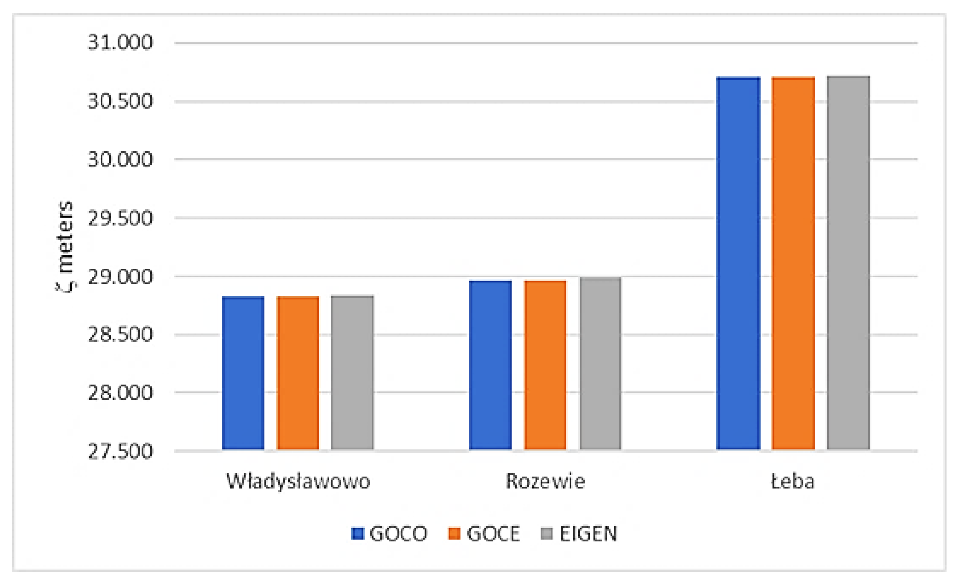
No	Name	ϕ			λ			GOCO	GOCE	EIGEN	Mean
		˚	‘	“	˚	‘	“
1	Władysławowo	54	47	48.324	18	25	7.493	28.824	28.830	28.838	28.831
2	Rozewie	54	49	46.1	18	20	7.9	28.968	28.966	28.993	28.976
3	Łeba	54	45	13.3	17	32	5.6	30.712	30.714	30.726	30.717

and Figure 11.

Comparisons have shown that quasigeoid anomalies at the tide gauge stations calculated from different geopotential models differ from 1 to 2 cm (Figure 11). The results based on the global satellite-only gravity field models GOCE and GOCO up to degree and order 300 have significantly increased the usability of satellite-only gravity field models for applications like height reference frame unification. This is of special value for areas with a lack of high-quality terrestrial gravity data.

The results of this work were also compared with the results obtained in the publication [49], p. 83, and we found that our results are 5 cm smaller at all tide gauge stations.

6. Conclusions

The computation of a regional gravimetric geoid model with proper accuracy is a difficult task that needs special notice and full investigation in all the phases of computations to produce good results.

Using this high-quality data set, we have carried out the gravimetric quasigeoid computation using the Helmert condensation method. This procedure is shown as an efficient method to compute in high resolution the new quasigeoid in the area 52° < λ < 68° and 11° < ϕ < 30° in a grid 1.5’ × 3.0’. Three versions of zero-tide quasigeoid were computed from the gravity data described above and geopotential models: GOCO06, GOCE-DIR6, and EIGEN-6C4.

Twenty-nine GNSS/leveling points of the ASG-EUPOS network were chosen for evaluating the quasigeoid models. According to the analyses carried out, their accuracy is on the level of ±4 cm. For reasons beyond our control, we have access to GNSS/leveling points at the southern end of the tested area, so we suspect that the accuracy of the calculated quasigeoid should be slightly higher about ±2 cm.

The gravity data used in this calculation come from different sources and differ in measurement methods, accuracy, and resolution. In addition, these data refer to different systems, both horizontal and vertical. We also did not have accurate information on gravity data tidal systems and terrain corrections (except in Finland, Sweden, and Poland) introduced into gravity anomalies. It is assumed that these data produced in the last century are in the mean tidal system and contain terrain corrections. Therefore, to calculate the new quasigeoid model in the Baltic, it is necessary to improve the quality of gravity data.

This work uses data only from airborne measurements and measurements at sea performed between 1978 and 1980 by the teams of the Moscow Research Institute. Therefore, the impact of additional data, e.g., sea data from Hakon Mossby or altimetric data on the accuracy of the quasigeoids to be calculated, should be investigated.

Finally, quasigeoid separation at the Władysławowo, Rozewie, and Ustka tide gauge stations was calculated. Differences between each geopotential model are from few millimeters to 1 centimeter. Then, the mean quasigeoid separations at tide gauge stations were compared with the value obtained in the paper [46], p. 83. Due to different methods in quasigeoid computations and different data sets used, the observed shift of 5 cm means a good agreement between these two solutions.

References

- Gruber, T.; Ågren, J.; Angermann, D.; Ellmann, A.; Engfeldt, A.; Gisinger, C.; Jaworski, L.; Marila, S.; Nastula, J.; Nilfouroushan, F.; et al. Geodetic SAR for Height System Unification and Sea Level Research—Observation Concept and Preliminary Results in the Baltic Sea. Remote. Sens. 2020, 12, 3747. [Google Scholar] [CrossRef]
- Torge, W. Geodesy, 3rd ed.; de Gruyter: New York, NY, USA, 2001. [Google Scholar]
- Sánchez, L.; Ågren, J.; Huang, J.; Wang, Y.M.; Mäkinetn, J.; Pail, R.; Barzaghi, R.; Vergos, G.S.; Ahlgren, K.; Liu, Q. Strategy for the realisation of the International Height Reference System (IHRS). J. Geod. 2021, 95, 33. [Google Scholar] [CrossRef]
- Tenzer, R.; Vaníček, P.; Santos, M.; Featherstone, W.E.; Kuhn, M. The rigorous determination of orthometric heights. J. Geod. 2005, 79, 82–92. [Google Scholar] [CrossRef] [Green Version]
- Featherstone, W.E.; Claessens, S.J. Closed-form transformation between geodetic and ellipsoidal coordinates. Stud. Geophys. Geod. 2008, 52, 1. [Google Scholar] [CrossRef] [Green Version]
- Ihde, J.; Augath, W.; Sacher, M. The Vertical Reference System for Europe. In Vertical Reference Systems. International Association of Geodesy Symposia; Springer: Berlin/Heidelberg, Germany, 2002; Volume 4249, pp. 345–350. [Google Scholar]
- Scharroo, R.; Visser, P. Precise orbit determination and gravity field improvement for the ERS satellites. J. Geophys. Res. Space Phys. 1998, 103, 8113–8127. [Google Scholar] [CrossRef]
- Tanni, L. The regional rise of the geoid in Central Europe. Ann. Acad. Sci. Fenn. Ser. A 1949, 3, 20. [Google Scholar]
- Jarmołowski, W. Determination of the Geoid Course in the Southern Baltic Sea Area from Marine and Aviation Gravimetric Observations and Satellite Altimetry (Published in Polish: Wyznaczenie przebiegu geoidy na obszarze południowego Morza Bałtyckiego z morskich i lotniczych obserwacji grawimetrycznych oraz altimetrii satelitarnej). Ph.D. Thesis, University of Warmia and Mazury in Olsztyn, Olsztyn, Poland, 2006. [Google Scholar]
- Kuczynska-Siehien, J.; Lyszkowicz, A.; Sideris, M.G. Evaluation of Altimetry Data in the Baltic Sea Region for Computation of New Quasigeoid Models over Poland. In Proceedings of the International Symposium on Advancing Geodesy in a Changing World, Kobe, Japan, 30 July–4 August 2017; International Association of Geodesy Symposia. Springer: Cham, Switzerland, 2019; Volume 149, pp. 51–60. [Google Scholar] [CrossRef]
- Forsberg, R.S.D. Geoid of the Nordic/Baltic region from surface/airborne gravimetry and GPS draping. In Proceedings of the International Symposium on Gravity, Geoid and Marine Geodesy, Tokyo, Japan, 30 September–5 October 1996; Springer: Berlin/Heidelberg, Germany, 1997; Volume 117, ISBN 3-540-63352-9. [Google Scholar]
- Ågren, J.; Strykowski, G.; Bilker-Koivula, M.; Omang, O.; Märdla, S.; Forsberg, R.; Ellmann, A.; Oja, T.; Liepins, I.; Parseliunas, E.; et al. The NKG2015 Gravimetric Geoid Model for the Nordic-Baltic Region. Available online: http://gghs2016.com/wp-content/uploads/2016/07/GGHS2016_paper_143.pdf (accessed on 20 April 2021).
- Ellmann, A. The Geoid for the Baltic Countries Determined by the Least-Squares Modification of Stokes’ Formula; Geodesy Report No 1061; Royal Institute of Technology, Department of Infrastructure: Stockholm, Sweden, 2004. [Google Scholar]
- Becker, J.J.; Sandwell, D.T.; Smith, W.; Braud, J.; Binder, B.; Depner, J.; Fabre, D.; Factor, J.; Ingalls, S.; Kim, S.-H.; et al. Global Bathymetry and Elevation Data at 30 Arc Seconds Resolution: SRTM30_PLUS. Mar. Geod. 2009, 32, 355–371. [Google Scholar] [CrossRef]
- Visser, P. Gravity field determination with GOCE and GRACE. Adv. Space Res. 1999, 23, 771–776. [Google Scholar] [CrossRef]
- Heiskanen, W.A.; Moritz, H. Physical Geodesy; W.H. Freeman and Company: San Francisco, CA, USA; Springer: Berlin/Heidelberg, Germany, 1967; Volume 41, pp. 491–492. [Google Scholar]
- Forsberg, R.; Tscherning, C.C. Topographic effects in gravity field modelling for BVP. Eng. Geol. Infrastruct. Plan. Eur. 2005, 239–272. [Google Scholar]
- Wichiencharoen, C. The Indirect Effects on the Computation of Geoid Undulation. Ohio State University, Department of Geodetic Science and Surveying, Report No. 336. 1982. Available online: http://www.ghbook.ir/index.php?name (accessed on 20 April 2021).
- Rapp, R.R. Methods for the Computations Detailed Geoid; Report No 233; Department of Geodetic Science, The Ohio State University: Columbus, OH, USA, 1975. [Google Scholar]
- Matsuo, K.; Forsberg, R. Gravimetric geoid computation over Colorado based on Remove–Compute–Restore Stokes–Helmert scheme. In Proceedings of the 27th International Union of Geodesy, Montréal, QC, Canada, 8–18 July 2019. [Google Scholar]
- Dahl, O.; Forsberg, R. Different ways to handle topography in practical geoid determination. Phys. Chem. Earth, Part A: Solid Earth Geod. 1999, 24, 41–46. [Google Scholar] [CrossRef]
- Forsberg, R.; Sideris, M.G. Geoid computations by the multi-band spherical FFT approach. Manuscr. Geod. 1993, 18, 82–90. [Google Scholar]
- Królikowski, C. Explanations to the Gravimetric Map of Poland 1:200,000 (Published in Polish: Objaśnienia do mapy grawimetrycznej Polski 1:200 000); Państwowy Instutut Geologiczny: Warszawa, Poland, 1994. [Google Scholar]
- Cisak, M.; Sas, A. Coordinates Transformation of Points from the “Borowa Góra” System to the “1942”. Available online: http://bc.igik.edu.pl/Content/147/PI_108_2004_2.pdf (accessed on 20 April 2021).
- Kryński, J. Precise Quasigeoid Modelling in Poland—Results and Accuracy Estimation (Published in Polish: Precyzyjne modelowanie quasigeoidy na obszarze Polski wyniki i ocena dokładności); Seria Monograficzna nr 13; Instytut Geodezji i Kartografii: Warsaw, Poland, 2007; ISBN 978-83-60024-11-9. [Google Scholar]
- Łyszkowicz, A. About the Problems Related to the Creation of a Uniform Heigh Reference System in the Region of the Baltic Sea (Published in Polish: O problemach związanych z tworzeniem jednolitego wysokościowego układu odniesienia w rejonie morza Bałtyckiego); First Continental Workshop on the Geoid in Europe; Published by Research Institute of Geodesy and Cartograph: Warszawa, Poland, 1992. [Google Scholar]
- Łyszkowicz, A. Description of the Geoid Survey Algorithm in Poland, Gravimetric and Height Data, Gravimetric Database GRAVBASE ver. 1-Altitude Reference System in the Baltic Sea Region (Published in Polish: Opis algorytmu badania geoidy na obszarze Polski, dane grawimetryczne i wysokościowe, grawimetryczna baza danych GRAVBASE ver. 1); Space Research Centre Polish Academy of Sciences: Warszawa, Poland, 1994. [Google Scholar]
- Kostiainen, M.K.J. On the accuracy of the gravity determined from the Bouguer anomaly register for leveling benchmarks. In Proceedings of the Second International Symposium on Problems Related to the Redefinition of North America Vertical Geodetic Networks (NAD Symposium), Ottawa, ON, Canada, 26–30 May 1980; pp. 525–536. [Google Scholar]
- Ekman, M. Impacts of geodynamic phenomena on systems for height and gravity. J. Geod. 1989, 63, 281–296. [Google Scholar] [CrossRef]
- Forsberg, R.; Olesen, A.V.; Keller, K.; Møller, M.; Gidskehaug, A.; Solheim, D. Airborne Gravity and Geoid Surveys in the Arctic and Baltic Seas. In Proceedings of the International Symposium on Kinematic Systems in Geodesy, Geomatics, and Navigation (KIS - 2001), Banff, AB, Canada, 5–8 June 2001; pp. 586–592. [Google Scholar]
- Fairhead, J. West-East European Gravity Project. 1995. Available online: https://www.earthdoc.org/content/papers/10.3997/2214-4609.201410155 (accessed on 20 April 2021).
- Pavlis, N.K.; Holmes, S.A.; Kenyon, S.C.; Factor, J.K. The development and evaluation of the Earth Gravitational Model 2008 (EGM2008). J. Geophys. Res. Space Phys. 2012, 117, 1–38. [Google Scholar] [CrossRef] [Green Version]
- Rülke, A.; Liebsch, G.; Sacher, M.; Schäfer, U.; Schirmer, U.; Ihde, J. Unification of European height system realizations. J. Geod. Sci. 2013, 2, 343–354. [Google Scholar] [CrossRef]
- Smith, W.H.F.; Sandwell, D.T. Global Sea Floor Topography from Satellite Altimetry and Ship Depth Soundings. Science 1997, 277, 1956–1962. [Google Scholar] [CrossRef] [Green Version]
- Schutz, B.E.; Zwally, H.J.; Shuman, C.A.; Hancock, D.; DiMarzio, J.P. Overview of the ICESat Mission. Geophys. Res. Lett. 2005, 32, L21S01. [Google Scholar] [CrossRef] [Green Version]
- Heck, B. An evaluation of some systematic error sources affecting terrestrial gravity anomalies. J. Geod. 1990, 64, 88–108. [Google Scholar] [CrossRef]
- Gatti, A.; Reguzzoni, M.; Venuti, G. The height datum problem and the role of satellite gravity models. J. Geod. 2012, 87, 15–22. [Google Scholar] [CrossRef]
- Bruinsma, S.L.; Förste, C.; Abrikosov, O.; Lemoine, J.-M.; Marty, J.-C.; Mulet, S.; Rio, M.-H.; Bonvalot, S. ESA’s satellite-only gravity field model via the direct approach based on all GOCE data. Geophys. Res. Lett. 2014, 41, 7508–7514. [Google Scholar] [CrossRef] [Green Version]
- Shako, R.; Förste, C.; Abrikosov, O.; Bruinsma, S.L.; Marty, J.-C.; Lemoine, J.-M.; Flechtner, F.; Neumayer, H.; Dahle, C. EIGEN-6C: A High-Resolution Global Gravity Combination Model Including GOCE Data. In Observation of the System Earth from Space—CHAMP, GRACE, GOCE and Future Missions; Advanced Technologies in Earth Sciences; Springer: Berlin/Heidelberg, Germany, 2013; pp. 155–161. [Google Scholar]
- Förste, C.; Bruinsma, S.L.; Abrikosov, O.; Lemoine, J.-M.; Schaller, T.; Götze, H.J. EIGEN-6C4 The latest combined global gravity field model including GOCE data up to degree and order 2190 of GFZ Postdam and GRGS Toulouse. In Proceedings of the 5th GOCE User Workshop, Paris, France, 22–28 November 2014. [Google Scholar]
- Kvas, A.; Brockmann, J.M.; Schubert, T.; Krauss, S.; Gruber, T.; Meyer, U.; Pail, R. A satellite-only global gravity field model. Earth Syst. Sci. Data 2020, 13, 99–118. [Google Scholar] [CrossRef]
- Bosy, J.; Graszka, W.; Oruba, A. ASG-EUPOS and the basic geodetic network in Poland (Published in Polish: ASG-EUPOS i podstawowa osnowa geodezyjna w Polsce). Biuletyn Wojskowej Akademii Technicznej 2010, 59, 7–15. [Google Scholar]
- Wyrzykowski, T. Monograph of the National 1st Class Precision Leveling Networks (Published in Polish: Monografia krajowych sieci niwelacji precyzyjnej I klasy); Published by Institute of Geodesy: Warszawa, Poland, 1988. [Google Scholar]
- Forsberg, R.; Tscherning, C. An Overview Manual for the GRAVSOFT Geodetic Gravity Field Modeling Programs. Contract Report for JUPEM 2008. Available online: http://scholar.google.com/scholar?hl=en&btnG=Search&q=intitle:An+overview+manual+for+the+GRAVSOFT+Geodetic+Gravity+Field+Modelling+Programs#0 (accessed on 28 April 2021).
- Available online: http://icgem.gfz-potsdam.de/home (accessed on 28 April 2021).
- Van Hees, G.S. Stokes formula using Fast Fourier Techniques. In Determination of the Geoid; International Association of Geodesy Symposia; Springer: Berlin/Heidelberg, Germany, 1991; Volume 106, pp. 405–408. [Google Scholar]
- Kadaj, R. Transformations between the height reference frames: Kronsztadt’60, PL-KRON86-NH, PL-EVRF2007-NH. Czasopismo Inżynierii Lądowej, Środowiska i Architektury 2018, 65, 5–24. [Google Scholar] [CrossRef]
- Kadaj, R.; Świętoń, T. Transpol v. 2.06; 2013; p. 45. Available online: https://docer.pl/doc/x1sxnvn (accessed on 26 May 2021).
- Gruber, T.; Oikonomidou, X.; Tum, D.A.; Dlr, C.G. BALTIC + Geodetic SAR for Baltic Height System Unification and Baltic Sea Level Research; Algorithm Theoretical Basis Document; SAR-HSU-AT-0013. Remote Sens. 2020, 12, 3747. [Google Scholar] [CrossRef]