
A Deep Detection Network Based on Interaction of Instance Segmentation and Object Detection for SAR Images


Abstract
:1. Introduction
2. Related Work
2.1. Traditional Ship Detection Methods
2.2. Object Detection Using CNNs
2.3. Ship Detection for Optical Remote Sensing Image
2.4. SAR Ship Detection with Deep Learning
3. Methodology
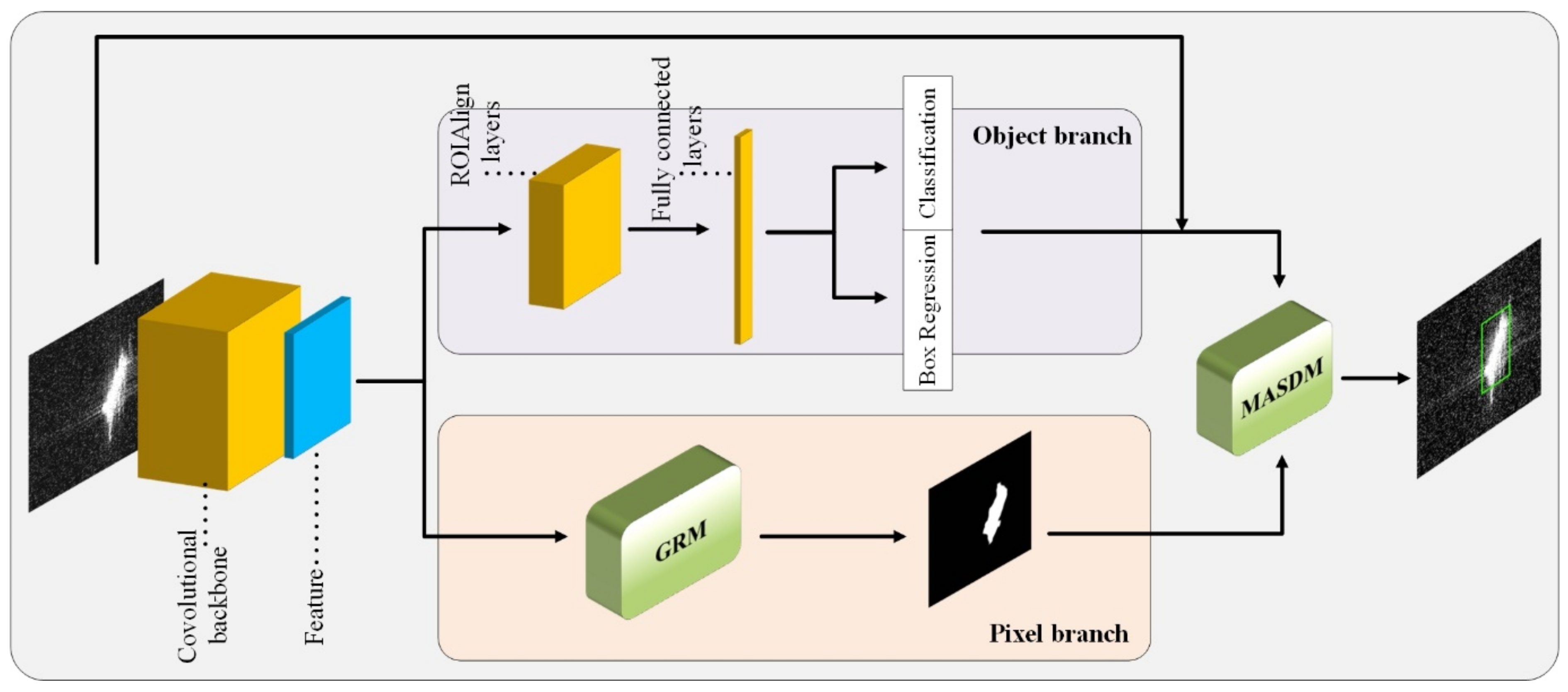
3.1. Architecture
3.2. Mask Extraction Strategy
3.2.1. Image Slices
3.2.2. Thresholding
3.2.3. Morphological Processing
3.2.4. Output Mask
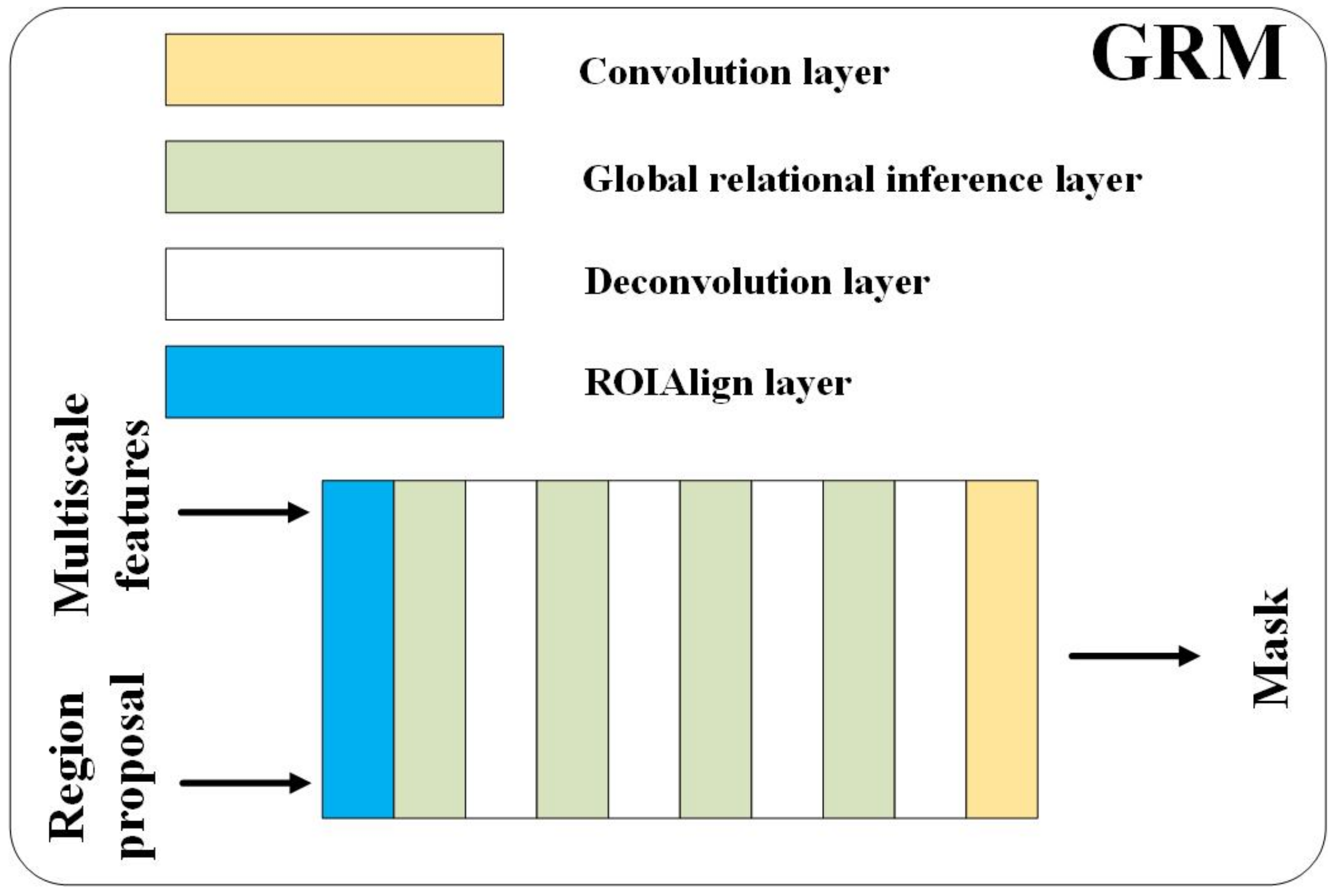
3.3. Global Reasoning Module
3.4. Mask Assisted Ship Detection Module
3.5. Loss Function
4. Experiments
4.1. Datasets and Evaluation Metrics
4.2. Experiment Results
4.2.1. Results on SAR-Ship-Dataset
4.2.2. Results on SSDD
4.3. Discussion
4.3.1. Ablation Experiment and Parameter Analysis
4.3.2. Performance Comparison
5. Conclusions
Author Contributions
Funding
Institutional Review Board Statement
Informed Consent Statement
Data Availability Statement
Conflicts of Interest
References
- Wu, Z.; Hou, B.; Jiao, L. Multiscale CNN With Autoencoder Regularization Joint Contextual Attention Network for SAR Image Classification. IEEE Trans. Geosci. Remote Sens. 2021, 59, 1200–1213. [Google Scholar] [CrossRef]
- Leng, X.; Ji, K.; Zhou, S.; Xing, X. Ship Detection Based on Complex Signal Kurtosis in Single-Channel SAR Imagery. IEEE Trans. Geosci. Remote Sens. 2019, 57, 6447–6461. [Google Scholar] [CrossRef]
- Chen, X.; Xiang, S.; Liu, C.; Pan, C. Vehicle Detection in Satellite Images by Hybrid Deep Convolutional Neural Networks. IEEE Geosci. Remote Sens. Lett. 2014, 11, 1797–1801. [Google Scholar] [CrossRef]
- Zhou, H.; Wei, L.; Lim, C.P.; Creighton, D.; Nahavandi, S. Robust Vehicle Detection in Aerial Images Using Bag-of-words and Orientation Aware Scanning. IEEE Trans. Geosci. Remote Sens. 2018, 56, 7074–7085. [Google Scholar] [CrossRef]
- Wang, Y.; Wang, C.; Zhang, H.; Dong, Y.; Wei, S. Automatic Ship Detection Based on RetinaNet Using Multi-Resolution Gaofen-3 Imagery. Remote Sens. 2019, 11, 531. [Google Scholar] [CrossRef] [Green Version]
- Liu, N.; Cao, Z.; Cui, Z.; Pi, Y.; Dang, S. Multi-Scale Proposal Generation for Ship Detection in SAR Images. Remote Sens. 2019, 11, 526. [Google Scholar] [CrossRef] [Green Version]
- Marino, A. A Notch Filter for Ship Detection with Polarimetric SAR Data. IEEE J. Sel. Top. Appl. Earth Observ. Remote Sens. 2013, 6, 1219–1232. [Google Scholar] [CrossRef] [Green Version]
- Wang, Y.; Liu, H. PolSAR Ship Detection Based on Superpixel-Level Scattering Mechanism Distribution Features. IEEE Geosci. Remote Sens. Lett. 2015, 12, 1780–1784. [Google Scholar] [CrossRef]
- Lin, H.; Chen, H.; Wang, H.; Yin, J.; Yang, J. Ship Detection for PolSAR Images via Task-Driven Discriminative Dictionary Learning. Remote Sens. 2019, 11, 769. [Google Scholar] [CrossRef] [Green Version]
- Robey, F.C.; Fuhrmann, D.R.; Kelly, E.J.; Nitzberg, R. A CFAR adaptive matched filter detector. IEEE Trans. Aerosp. Electron. Syst. 1992, 28, 208–216. [Google Scholar] [CrossRef] [Green Version]
- He, K.; Zhang, X.; Ren, S.; Sun, J. Spatial Pyramid Pooling in Deep Convolutional Networks for Visual Recognition. IEEE Trans. Pattern Anal. Mach. Intell. 2015, 37, 1904–1916. [Google Scholar] [CrossRef] [PubMed] [Green Version]
- Shin, H.C.; Roth, H.R.; Gao, M.; Lu, L.; Xu, Z.; Nogues, I.; Yao, J.; Mollura, D.; Summers, R.M. Deep Convolutional Neural Networks for Computer-Aided Detection: CNN Architectures, Dataset Characteristics and Transfer Learning. IEEE Trans. Med. Imaging 2016, 35, 1285–1298. [Google Scholar] [CrossRef] [PubMed] [Green Version]
- Ji, S.; Xu, W.; Yang, M.; Yu, K. 3D Convolutional Neural Networks for Human Action Recognition. IEEE Trans. Pattern Anal. Mach. Intell. 2013, 35, 221–231. [Google Scholar] [CrossRef] [PubMed] [Green Version]
- Redmon, J.; Divvala, S.; Girshick, R.; Farhadi, A. You only look once: Unified, real-time object detection. In Proceedings of the IEEE Conference on Computer Vision and Pattern Recognition (CVPR), Las Vegas, NV, USA, 27–30 June 2016. [Google Scholar]
- Liu, W.; Anguelov, D.; Erhan, D.; Szegedy, C.; Reed, S.; Fu, C.; Berg, A.C. SSD: Single shot multibox detector. In Proceedings of the European Conference on Computer Vision (ECCV), Amsterdam, The Netherlands, 8–16 October 2016; pp. 21–37. [Google Scholar]
- Girshick, R.; Donahue, J.; Darrell, T.; Malik, J. Region-based convolutional networks for accurate object detection and segmentation. IEEE Trans. Pattern Anal. Mach. Intell. 2016, 38, 142–158. [Google Scholar] [CrossRef]
- Girshick, R.B. Fast R-CNN. In Proceedings of the IEEE International Conference on Computer Vision (ICCV), Santiago, Chile, 7–13 December 2015; pp. 1440–1448. [Google Scholar]
- Cui, Z.; Li, Q.; Cao, Z.; Liu, N. Dense Attention Pyramid Networks for Multi-Scale Ship Detection in SAR Images. IEEE Trans. Geosci. Remote Sens. 2019, 57, 8983–8997. [Google Scholar] [CrossRef]
- Wang, S.; Gong, Y.; Xing, J.; Huang, L.; Huang, C.; Hu, W. RDSNet: A New Deep Architecture for Reciprocal Object Detection and Instance Segmentation. In Proceedings of the Association for the Advancement of Artificial Intelligence (AAAI), New York, NY, USA, 7–12 February 2020; pp. 12208–12215. [Google Scholar]
- He, K.; Gkioxari, G.; Dollar, P.; Girshick, R. Mask R-CNN. In Proceedings of the IEEE International Conference on Computer Vision (ICCV), Venice, Italy, 22–29 October 2017; pp. 2980–2988. [Google Scholar]
- Wang, Y.; Liu, H. A Hierarchical Ship Detection Scheme for High-Resolution SAR Images. IEEE Trans. Geosci. Remote Sens. 2012, 50, 4173–4184. [Google Scholar] [CrossRef]
- Gao, G. A Parzen-Window-Kernel-Based CFAR Algorithm for Ship Detection in SAR Images. IEEE Geosci. Remote Sens. Lett. 2011, 8, 557–561. [Google Scholar] [CrossRef]
- An, W.; Xie, C.; Yuan, X. An Improved Iterative Censoring Scheme for CFAR Ship Detection with SAR Imagery. IEEE Trans. Geosci. Remote Sens. 2014, 52, 4585–4595. [Google Scholar]
- Li, T.; Liu, Z.; Xie, R.; Ran, L. An Improved Superpixel-Level CFAR Detection Method for Ship Targets in High-Resolution SAR Images. IEEE J. Sel. Top. Appl. Earth Observ. Remote Sens. 2018, 11, 184–194. [Google Scholar] [CrossRef]
- Gao, G.; Gao, S.; He, J.; Li, G. Adaptive Ship Detection in Hybrid-Polarimetric SAR Images Based on the Power–Entropy Decomposition. IEEE Trans. Geosci. Remote Sens. 2018, 56, 5394–5407. [Google Scholar] [CrossRef]
- Lang, H.; Xi, Y.; Zhang, X. Ship Detection in High-Resolution SAR Images by Clustering Spatially Enhanced Pixel Descriptor. IEEE Trans. Geosci. Remote Sens. 2019, 57, 5407–5423. [Google Scholar] [CrossRef]
- Pastina, D.; Fico, F.; Lombardo, P. Detection of ship targets in COSMO-SkyMed SAR images. In Proceedings of the IEEE Radar Conference (RADAR), Kansas City, MO, USA, 23–27 May 2011; pp. 928–933. [Google Scholar]
- Le, Q.V.; Ngiam, J.; Coates, A.; Lahiri, A.; Prochnow, B.; Ng, A.Y. On optimization methods for deep learning. In Proceedings of the International Conference on Machine Learning (ICML), Bellevue, WA, USA, 28 June–2 July 2011; pp. 265–272. [Google Scholar]
- Le, Q.V.; Zou, W.Y.; Yeung, S.Y.; Ng, A.Y. Learning hierarchical invariant spatio-temporal features for action recognition with independent subspace analysis. In Proceedings of the IEEE Conference on Computer Vision and Pattern Recognition (CVPR), Colorado Springs, CO, USA, 21–23 June 2011; pp. 3361–3368. [Google Scholar]
- Messina, M.; Greco, M.; Fabbrini, L.; Pinelli, G. Modified Otsu’s algorithm: A new computationally efficient ship detection algorithm for SAR images. In Proceedings of the Tyrrhenian Workshop on Advances in Radar and Remote Sensing (TyWRRS), Naples, Italy, 12–14 September 2012; pp. 262–266. [Google Scholar]
- Ouchi, K.; Tamaki, S.; Yaguchi, H.; Iehara, M. Ship Detection Based on Coherence Images Derived From Cross Correlation of Multilook SAR Images. IEEE Geosci. Remote Sens. Lett. 2004, 1, 184–187. [Google Scholar] [CrossRef]
- Tello, M.; Martinez, C.L.; Mallorqui, J.J. A Novel Algorithm for Ship Detection in SAR Imagery Based on the Wavelet Transform. IEEE Geosci. Remote Sens. Lett. 2005, 2, 201–205. [Google Scholar] [CrossRef]
- Bochkovskiy, A.; Wang, C.Y.; Liao, H. YOLOv4: Optimal Speed and Accuracy of Object Detection. arXiv 2020, arXiv:2004.10934v1. [Google Scholar]
- Simonyan, K.; Zisserman, A. Very deep convolutional networks for large-scale image recognition. In Proceedings of the International Conference on Learning Representations (ICLR), San Diego, CA, USA, 7–9 May 2015. [Google Scholar]
- He, K.; Zhang, X.; Ren, S.; Sun, J. Deep Residual Learning for Image Recognition. In Proceedings of the IEEE Conference on Computer Vision and Pattern Recognition (CVPR), Las Vegas, NV, USA, 27–30 June 2016; pp. 770–778. [Google Scholar]
- Huang, G.; Liu, Z.; Maaten, L.V.D.; Weinberger, K.Q. Densely Connected Convolutional Networks. In Proceedings of the IEEE Conference on Computer Vision and Pattern Recognition (CVPR), Honolulu, HI, USA, 22–25 July 2017; pp. 2261–2269. [Google Scholar]
- Ren, S.; He, K.; Girshick, R.; Sun, J. Faster R-CNN: Towards Real-Time Object Detection with Region Proposal Networks. IEEE Trans. Pattern Anal. Mach. Intell. 2017, 39, 1137–1149. [Google Scholar] [CrossRef] [Green Version]
- Lin, T.Y.; Goyal, P.; Girshick, R.; He, K.; Dollar, P. Focal Loss for Dense Object Detection. IEEE Trans. Pattern Anal. Mach. Intell. 2020, 42, 318–327. [Google Scholar] [CrossRef] [Green Version]
- Lin, T.Y.; Dollar, P.; Girshick, R.; He, K.; Hariharan, B.; Belongie, S. Feature Pyramid Networks for Object Detection. In Proceedings of the IEEE Conference on Computer Vision and Pattern Recognition (CVPR), Honolulu, HI, USA, 22–25 July 2017; pp. 936–944. [Google Scholar]
- Liu, S.; Qi, L.; Qin, H.; Shi, J.; Jia, J. Path Aggregation Network for Instance Segmentation. In Proceedings of the IEEE Conference on Computer Vision and Pattern Recognition (CVPR), Salt Lake City, UT, USA, 18–22 June 2018; pp. 8759–8768. [Google Scholar]
- Wu, F.; Zhou, Z.; Wang, B.; Ma, J. Inshore Ship Detection Based on Convolutional Neural Network in Optical Satellite Images. IEEE J. Sel. Top. Appl. Earth Observ. Remote Sens. 2018, 11, 4005–4015. [Google Scholar] [CrossRef]
- Yan, Y.; Tan, Z.; Su, N. A Data Augmentation Strategy Based on Simulated Samples for Ship Detection in RGB Remote Sensing Images. ISPRS Int. J. Geo-Inf. 2019, 8, 276. [Google Scholar] [CrossRef] [Green Version]
- Li, L.; Zhou, Z.; Wang, B.; Miao, L.; Zong, H. A Novel CNN-Based Method for Accurate Ship Detection in HR Optical Remote Sensing Images via Rotated Bounding Box. IEEE Trans. Geosci. Remote Sens. 2021, 59, 686–699. [Google Scholar] [CrossRef]
- Liu, Q.; Xiang, X.; Yang, Z.; Hu, Y.; Hong, Y. Arbitrary Direction Ship Detection in Remote-Sensing Images Based on Multitask Learning and Multiregion Feature Fusion. IEEE Trans. Geosci. Remote Sens. 2021, 59, 1553–1564. [Google Scholar] [CrossRef]
- Ma, J.; Zhou, Z.; Wang, B.; Zong, H.; Wu, F. Ship Detection in Optical Satellite Images via Directional Bounding Boxes Based on Ship Center and Orientation Prediction. Remote Sens. 2019, 11, 2173. [Google Scholar] [CrossRef] [Green Version]
- Feng, Y.; Diao, W.; Sun, X.; Yan, M.; Gao, X. Towards Automated Ship Detection and Category Recognition from High-Resolution Aerial Images. Remote Sens. 2019, 11, 1901. [Google Scholar] [CrossRef] [Green Version]
- Fan, W.; Zhou, F.; Bai, X.; Tao, M.; Tian, T. Ship Detection Using Deep Convolutional Neural Networks for PolSAR Images. Remote Sens. 2019, 11, 2862. [Google Scholar] [CrossRef] [Green Version]
- Fan, Q.; Chen, F.; Cheng, M.; Lou, S.; Xiao, R.; Zhang, B.; Wang, C.; Li, J. Ship Detection Using a Fully Convolutional Network with Compact Polarimetric SAR Images. Remote Sens. 2019, 11, 2171. [Google Scholar] [CrossRef] [Green Version]
- Gao, F.; Shi, W.; Wang, J.; Yang, E.; Zhou, H. Enhanced Feature Extraction for Ship Detection from Multi-Resolution and Multi-Scene Synthetic Aperture Radar (SAR) Images. Remote Sens. 2019, 11, 2694. [Google Scholar] [CrossRef] [Green Version]
- Wei, S.; Su, H.; Ming, J.; Wang, C.; Yan, M.; Kumar, D.; Shi, J.; Zhang, X. Precise and Robust Ship Detection for High-Resolution SAR Imagery Based on HR-SDNet. Remote Sens. 2020, 12, 167. [Google Scholar] [CrossRef] [Green Version]
- Chen, C.; He, C.; Hu, C.; Pei, H.; Jiao, L. MSARN: A Deep Neural Network Based on an Adaptive Recalibration Mechanism for Multiscale and Arbitrary-Oriented SAR Ship Detection. IEEE Access 2019, 7, 159262–159283. [Google Scholar] [CrossRef]
- Hou, B.; Ren, Z.; Zhao, W.; Wu, Q.; Jiao, L. Object Detection in High-Resolution Panchromatic Images Using Deep Models and Spatial Template Matching. IEEE Trans. Geosci. Remote Sens. 2019, 58, 956–970. [Google Scholar] [CrossRef]
- Kang, M.; Leng, X.; Lin, Z.; Ji, K. A Modified Faster R-CNN Based on CFAR Algorithm for SAR Ship Detection. In Proceedings of the 2017 International Workshop on Remote Sensing with Intelligent Processing (RSIP), Shanghai, China, 18–21 May 2017. [Google Scholar]
- Zou, L.; Zhang, H.; Wang, C.; Wu, F.; Gu, F. MW-ACGAN: Generating Multiscale High-Resolution SAR Images for Ship Detection. Sensors 2020, 20, 6673. [Google Scholar] [CrossRef]
- Ridler, T.W.; Calvard, S. Picture Thresholding Using an Iterative Selection Method. IEEE Trans. Syst. 1978, 8, 630–632. [Google Scholar]
- Monsalve, A.F.T.; Medina, J.V. Hardware implementation of ISODATA and Otsu thresholding algorithms. In Proceedings of the IEEE Symposium on Signal Processing, Images and Artificial Vision (STSIVA), Bucaramanga, DC, USA, 31 August–2 September 2016. [Google Scholar]
- Chen, Y.; Rohrbach, M.; Yan, Z.; Shuicheng, Y.; Feng, J.; Kalantidis, Y. Graph-Based Global Reasoning Networks. In Proceedings of the IEEE Conference on Computer Vision and Pattern Recognition (CVPR), Long Beach, CA, USA, 15–21 June 2019; pp. 433–442. [Google Scholar]
- Kipf, T.; Welling, M. Semi-Supervised Classification with Graph Convolutional Networks. arXiv 2017, arXiv:1609.02907. [Google Scholar]
- Wang, Y.; Wang, C.; Zhang, H.; Dong, Y.; Wei, S. A SAR Dataset of Ship Detection for Deep Learning under Complex Backgrounds. Remote Sens. 2019, 11, 765. [Google Scholar] [CrossRef] [Green Version]
- Li, J.; Qu, C.; Shao, J. Ship detection in SAR images based on an improved faster R-CNN. In Proceedings of the SAR in Big Data Era (BIGSARDATA), Beijing, China, 13–14 November 2017. [Google Scholar]
- Lin, T.Y.; Maire, M.; Belongie, S.; Bourdev, L.; Girshick, R.; Hays, J.; Perona, P.; Ramanan, D.; Zitnick, C.L.; Dollar, P. Microsoft COCO: Common Objects in Context. In Proceedings of the 13th European Conference, Zurich, Switzerland, 6–12 September 2014. [Google Scholar]
- Zhao, Q.; Sheng, T.; Wang, Y.; Tang, Z.; Chen, Y.; Cai, L.; Ling, H. M2Det: A Single-Shot Object Detector Based on Multi-Level Feature Pyramid Network. In Proceedings of the Association for the Advancement of Artificial Intelligence (AAAI), Honolulu, HI, USA, 27 January–1 February 2019; pp. 9259–9266. [Google Scholar]
- Zhang, S.; Wen, L.; Bian, X.; Lei, Z.; Li, S.Z. Single-Shot Refinement Neural Network for Object Detection. In Proceedings of the IEEE Conference on Computer Vision and Pattern Recognition (CVPR), Salt Lake City, UT, USA, 18–22 June 2018; pp. 4203–4212. [Google Scholar]
- Cao, J.; Cholakkal, H.; Anwer, R.M.; Khan, F.S.; Pang, Y.; Shao, L. D2Det: Towards High Quality Object Detection and Instance Segmentation. In Proceedings of the IEEE Conference on Computer Vision and Pattern Recognition (CVPR), Online, 14–19 June 2020. [Google Scholar]
- Niemenlehto, P.H.; Juhola, M. Application of the Cell Averaging Constant False Alarm Rate Technique to Saccade Detection in Electro-oculography. In Proceedings of the 29th Annual International Conference of the IEEE Engineering in Medicine and Biology Society, Lyon, France, 22–26 August 2007. [Google Scholar]
- Hou, B.; Yang, W.; Wang, S.; Hou, X. SAR image ship detection based on visual attention model. In Proceedings of the 2013 IEEE International Geoscience and Remote Sensing Symposium (IGARSS), Melbourne, Australia, 21–26 July 2013. [Google Scholar]


| Metric | Meaning |
|---|---|
| AP | AP at IOU = 0.50:0.05:0.95 |
| AP50 | AP at IOU = 0.50 |
| AP75 | AP at IOU = 0.75 |
| APS | AP for small objects: area < 322 (IOU = 0.50:0.05:0.95) |
| APM | AP for medium objects: 322 < area < 962 (IOU = 0.50:0.05:0.95) |
| APL | AP for large objects: area > 962 (IOU = 0.50:0.05:0.95) |
| AP | AP50 | AP75 | APS | APM | APL | |
|---|---|---|---|---|---|---|
| faster-rcnn + r50 | 0.586 | 0.944 | 0.669 | 0.557 | 0.631 | 0.646 |
| faster-rcnn + r101 | 0.569 | 0.917 | 0.627 | 0.586 | 0.543 | 0.460 |
| mask-rcnn + r50 | 0.448 | 0.852 | 0.540 | 0.452 | 0.439 | 0.351 |
| mask-rcnn + r101 | 0.433 | 0.851 | 0.543 | 0.429 | 0.441 | 0.382 |
| YOLOv3 | 0.359 | 0.760 | 0.356 | 0.377 | 0.339 | 0.227 |
| YOLOv4 | 0.596 | 0.954 | 0.669 | 0.597 | 0.589 | 0.592 |
| SSD | 0.343 | 0.755 | 0.397 | 0.327 | 0.368 | 0.325 |
| RefineDet | 0.450 | 0.888 | 0.572 | 0.464 | 0.427 | 0.224 |
| M2Det | 0.372 | 0.836 | 0.413 | 0.437 | 0.312 | 0.259 |
| D2Det | 0.591 | 0.948 | 0.671 | 0.597 | 0.587 | 0.581 |
| ISASDNet + r50 | 0.601 | 0.953 | 0.652 | 0.615 | 0.582 | 0.544 |
| ISASDNet + r101 | 0.596 | 0.958 | 0.694 | 0.609 | 0.587 | 0.578 |
| Method | CA-CFAR | VAM | ISASDNet with ResNet50 | ISASDNet with ResNet101 |
|---|---|---|---|---|
| FoM | 0.1103 | 0.1691 | 0.6287 | 0.6515 |
| AP | AP50 | AP75 | APS | APM | APL | |
|---|---|---|---|---|---|---|
| faster-rcnn + r50 | 0.587 | 0.947 | 0.629 | 0.609 | 0.561 | 0.477 |
| faster-rcnn + r101 | 0.579 | 0.956 | 0.618 | 0.593 | 0.552 | 0.490 |
| mask-rcnn + r50 | 0.557 | 0.927 | 0.585 | 0.571 | 0.522 | 0.489 |
| mask-rcnn + r101 | 0.563 | 0.921 | 0.589 | 0.588 | 0.525 | 0.463 |
| YOLOv3 | 0.508 | 0.909 | 0.546 | 0.534 | 0.458 | 0.474 |
| YOLOv4 | 0.601 | 0.960 | 0.674 | 0.616 | 0.594 | 0.579 |
| SSD | 0.481 | 0.865 | 0.520 | 0.511 | 0.437 | 0.407 |
| RefineDet | 0.588 | 0.949 | 0.598 | 0.610 | 0.563 | 0.530 |
| M2Det | 0.498 | 0.903 | 0.531 | 0.531 | 0.462 | 0.410 |
| D2Det | 0.594 | 0.955 | 0.643 | 0.599 | 0.582 | 0.586 |
| ISASDNet + r50 | 0.610 | 0.954 | 0.677 | 0.624 | 0.605 | 0.552 |
| ISASDNet + r101 | 0.627 | 0.968 | 0.685 | 0.636 | 0.603 | 0.525 |
| Method | CA-CFAR | VAM | ISASDNet with ResNet50 | ISASDNet with ResNet101 |
|---|---|---|---|---|
| FoM | 0.1981 | 0.2317 | 0.6558 | 0.6632 |
| AP | AP50 | AP75 | APS | APM | APL | |
|---|---|---|---|---|---|---|
| Case 1 | 0.448 | 0.852 | 0.540 | 0.452 | 0.439 | 0.351 |
| Case 2 | 0.461 | 0.845 | 0.525 | 0.476 | 0.450 | 0.448 |
| Case 3 | 0.567 | 0.924 | 0.611 | 0.538 | 0.582 | 0.471 |
| Case 4 | 0.601 | 0.953 | 0.652 | 0.615 | 0.593 | 0.544 |
| Method | Faster-rcnn + r50 | Faster-rcnn + r101 | Mask-rcnn + r50 | Mask-rcnn + r101 |
|---|---|---|---|---|
| Time | 0.22546 | 0.28357 | 0.23263 | 0.29853 |
| Method | YOLOv3 | YOLOv4 | SSD | RefineDet |
| Time | 0.07052 | 0.08459 | 0.07475 | 0.08306 |
| Method | M2Det | D2Det | ISASDNet + r50 | ISASDNet + r101 |
| Time | 0.09623 | 0.24690 | 0.43848 | 0.44733 |
| Data Volume | Methods | AP | AP50 | AP75 |
|---|---|---|---|---|
| 55% | faster-rcnn + r50 | 0.551 | 0.929 | 0.620 |
| faster-rcnn + r101 | 0.529 | 0.889 | 0.594 | |
| mask-rcnn + r50 | 0.428 | 0.836 | 0.520 | |
| mask-rcnn + r101 | 0.399 | 0.794 | 0.513 | |
| YOLOv3 | 0.268 | 0.604 | 0.184 | |
| YOLOv4 | 0.549 | 0.929 | 0.612 | |
| SSD | 0.328 | 0.739 | 0.381 | |
| RefineDet | 0.429 | 0.849 | 0.537 | |
| M2Det | 0.354 | 0.787 | 0.382 | |
| D2Det | 0.551 | 0.919 | 0.621 | |
| ISASDNet + r50 | 0.585 | 0.931 | 0.621 | |
| ISASDNet + r101 | 0.585 | 0.939 | 0.651 | |
| 60% | faster-rcnn + r50 | 0.558 | 0.925 | 0.624 |
| faster-rcnn + r101 | 0.545 | 0.905 | 0.603 | |
| mask-rcnn + r50 | 0.437 | 0.845 | 0.527 | |
| mask-rcnn + r101 | 0.405 | 0.813 | 0.521 | |
| YOLOv3 | 0.270 | 0.612 | 0.179 | |
| YOLOv4 | 0.561 | 0.940 | 0.628 | |
| SSD | 0.335 | 0.746 | 0.389 | |
| RefineDet | 0.439 | 0.856 | 0.551 | |
| M2Det | 0.365 | 0.809 | 0.394 | |
| D2Det | 0.566 | 0.925 | 0.640 | |
| ISASDNet + r50 | 0.588 | 0.945 | 0.635 | |
| ISASDNet + r101 | 0.590 | 0.944 | 0.676 | |
| 65% | faster-rcnn + r50 | 0.567 | 0.932 | 0.643 |
| faster-rcnn + r101 | 0.558 | 0.910 | 0.618 | |
| mask-rcnn + r50 | 0.449 | 0.853 | 0.542 | |
| mask-rcnn + r101 | 0.429 | 0.836 | 0.535 | |
| YOLOv3 | 0.291 | 0.625 | 0.217 | |
| YOLOv4 | 0.588 | 0.947 | 0.639 | |
| SSD | 0.339 | 0.754 | 0.397 | |
| RefineDet | 0.447 | 0.868 | 0.562 | |
| M2Det | 0.370 | 0.821 | 0.403 | |
| D2Det | 0.583 | 0.933 | 0.647 | |
| ISASDNet + r50 | 0.592 | 0.949 | 0.643 | |
| ISASDNet + r101 | 0.596 | 0.951 | 0.684 |
| Noise Variance | Methods | AP | AP50 | AP75 |
|---|---|---|---|---|
| 0.1 | faster-rcnn + r50 | 0.523 | 0.888 | 0.566 |
| faster-rcnn + r101 | 0.523 | 0.895 | 0.561 | |
| mask-rcnn + r50 | 0.377 | 0.805 | 0.469 | |
| mask-rcnn + r101 | 0.369 | 0.806 | 0.450 | |
| YOLOv3 | 0.235 | 0.584 | 0.137 | |
| YOLOv4 | 0.546 | 0.904 | 0.592 | |
| SSD | 0.209 | 0.507 | 0.102 | |
| RefineDet | 0.389 | 0.814 | 0.497 | |
| M2Det | 0.365 | 0.796 | 0.461 | |
| D2Det | 0.546 | 0.902 | 0.585 | |
| ISASDNet + r50 | 0.557 | 0.921 | 0.633 | |
| ISASDNet + r101 | 0.559 | 0.928 | 0.648 | |
| 0.2 | faster-rcnn + r50 | 0.511 | 0.881 | 0.540 |
| faster-rcnn + r101 | 0.508 | 0.893 | 0.524 | |
| mask-rcnn + r50 | 0.365 | 0.799 | 0.452 | |
| mask-rcnn + r101 | 0.362 | 0.791 | 0.448 | |
| YOLOv3 | 0.153 | 0.404 | 0.088 | |
| YOLOv4 | 0.513 | 0.893 | 0.559 | |
| SSD | 0.236 | 0.602 | 0.158 | |
| RefineDet | 0.408 | 0.841 | 0.492 | |
| M2Det | 0.362 | 0.802 | 0.466 | |
| D2Det | 0.526 | 0.902 | 0.581 | |
| ISASDNet + r50 | 0.538 | 0.907 | 0.605 | |
| ISASDNet + r101 | 0.542 | 0.911 | 0.629 | |
| 0.3 | faster-rcnn + r50 | 0.491 | 0.870 | 0.503 |
| faster-rcnn + r101 | 0.482 | 0.873 | 0.486 | |
| mask-rcnn + r50 | 0.348 | 0.782 | 0.425 | |
| mask-rcnn + r101 | 0.351 | 0.782 | 0.434 | |
| YOLOv3 | 0.169 | 0.435 | 0.093 | |
| YOLOv4 | 0.503 | 0.873 | 0.497 | |
| SSD | 0.201 | 0.563 | 0.139 | |
| RefineDet | 0.398 | 0.821 | 0.454 | |
| M2Det | 0.341 | 0.773 | 0.417 | |
| D2Det | 0.508 | 0.868 | 0.500 | |
| ISASDNet + r50 | 0.519 | 0.886 | 0.588 | |
| ISASDNet + r101 | 0.518 | 0.891 | 0.593 |
Publisher’s Note: MDPI stays neutral with regard to jurisdictional claims in published maps and institutional affiliations. |
© 2021 by the authors. Licensee MDPI, Basel, Switzerland. This article is an open access article distributed under the terms and conditions of the Creative Commons Attribution (CC BY) license (https://creativecommons.org/licenses/by/4.0/).
Share and Cite
Wu, Z.; Hou, B.; Ren, B.; Ren, Z.; Wang, S.; Jiao, L. A Deep Detection Network Based on Interaction of Instance Segmentation and Object Detection for SAR Images. Remote Sens. 2021, 13, 2582. https://doi.org/10.3390/rs13132582
Wu Z, Hou B, Ren B, Ren Z, Wang S, Jiao L. A Deep Detection Network Based on Interaction of Instance Segmentation and Object Detection for SAR Images. Remote Sensing. 2021; 13(13):2582. https://doi.org/10.3390/rs13132582
Chicago/Turabian StyleWu, Zitong, Biao Hou, Bo Ren, Zhongle Ren, Shuang Wang, and Licheng Jiao. 2021. "A Deep Detection Network Based on Interaction of Instance Segmentation and Object Detection for SAR Images" Remote Sensing 13, no. 13: 2582. https://doi.org/10.3390/rs13132582
APA StyleWu, Z., Hou, B., Ren, B., Ren, Z., Wang, S., & Jiao, L. (2021). A Deep Detection Network Based on Interaction of Instance Segmentation and Object Detection for SAR Images. Remote Sensing, 13(13), 2582. https://doi.org/10.3390/rs13132582