Abstract
The mode-1 semidiurnal internal tides that emanate from multiple sources in the Sulu-Sulawesi Seas are investigated using multi-satellite altimeter data from 1993–2020. A practical plane-wave analysis method is used to separately extract multiple coherent internal tides, with the nontidal noise in the internal tide field further removed by a two-dimensional (2-D) spatial band-pass filter. The complex radiation pathways and interference patterns of the internal tides are revealed, showing a spatial contrast between the Sulu Sea and the Sulawesi Sea. The mode-1 semidiurnal internal tides in the Sulawesi Sea are effectively generated from both the Sulu and Sangihe Island chains, forming a spatially inhomogeneous interference pattern in the deep basin. A cylindrical internal tidal wave pattern from the Sibutu passage is confirmed for the first time, which modulates the interference pattern. The interference field can be reproduced by a line source model. A weak reflected internal tidal beam off the Sulawesi slope is revealed. In contrast, the Sulu Island chain is the sole energetic internal tide source in the Sulu Sea, thus featuring a relatively consistent wave and energy flux field in the basin. These energetic semidiurnal internal tidal beams contribute to the frequent occurrence of internal solitary waves (ISWs) in the study area. On the basis of the 28-year consistent satellite measurements, the northward semidiurnal tidal energy flux from the Sulu Island chain is 0.46 GW, about 25% of the southward energy flux. For M2, the altimetric estimated energy fluxes from the Sulu Island chain are about 80% of those from numerical simulations. The total semidiurnal tidal energy flux from the Sulu and Sangihe Island chains into the Sulawesi Sea is about 2.7 GW.
1. Introduction
Internal tides are widespread in the stratified ocean and act as a significant part in the energy cascade of multiscale oceanic processes. They are generated by the flux of barotropic tidal currents over complex bathymetries, such as the seamounts, trenches, ridges, and continental slopes. The globally integrated barotropic into baroclinic conversion rate in the deep ocean is estimated at ~1 TW [1]. The long-range radiation of internal tides in the open ocean is relevant to low modes that emanate from the generation sites [2]. The breaking of internal tides can cause energetic tidal mixing, which is essential to drive the large-scale meridional overturning circulation (MOC) and, subsequently, to affect the climate variability [3].
The propagation of internal tides redistributes the baroclinic tidal energy across the ocean basin, which is closely related to the inhomogeneous distribution of deep-sea mixing [4]. In particular, the semidiurnal internal tides dominate the tidal energy transfer process in the deep ocean and balance the global internal tide energy budget [5]. A correct characterization of the propagation paths and directions of the internal tidal energy flux will significantly contribute to parameterizing realistic diapycnal mixing in the ocean models [6]. However, the horizontal inhomogeneity in the energy flux density largely modulated by the interference of internal tides remains unknown [7]. Both the numerical models and satellite altimetry have revealed the widespread presence of multiwave interferences in the open ocean [8]. Therefore, it is crucial to regionally characterize multisource internal tides among the world ocean’s hotspots [9,10,11,12], based on a combination of simulations and multi-platform observations.
The Indonesian Archipelago acts as the only tropical connection of the Pacific and Indian Oceans and features the most complicated topography among the world’s regional seas. It is identified as an energetic internal tide generation field in the global ocean based on in situ measurements, numerical model simulations, and satellite altimeters [4,8,13]. The internal tide source regions include the Manipa, Lifamatola, Lombok, and Ombai Straits, and the Sulu and Sangihe Island chains et al. Previous studies showed that internal tides in different sea areas interact with each other, and internal tide fractions of different cycles interact nonlinearly, forming extremely complex and variable internal tide fields [14,15]. Koch-Larrouy et al. [16] showed numerically that tidal mixing has a considerable effect on the tropical climate system. The tidal mixing influences the SST patterns in the Indonesian Seas and changes the character of the Indonesian Throughflow (ITF) [17,18]. To date, much work on internal tides in the Indonesian Archipelago has been made based on numerical simulations. However, the verification of models remains limited due to insufficient field observations.
In the last two decades, satellite altimetry has been widely used as an important method to observe internal tides [19,20,21]. A recent M2 internal tide prediction model on a global scale without blind directions was constructed using multiple satellite altimeter measurements [22]. In addition, Zaron [21] filtered the main mesoscale noise and proposed global internal tide fields for the diurnal constituent (O1 and K1) and the semidiurnal constituent (M2 and S2). The radiation and propagation of internal tides have been investigated in numerous marginal oceans by satellite observations [23,24]. In the regions where in situ measurements are lacking, satellite altimeter measurements can be utilized to reveal a broad distribution of internal tide signals. Note that most existing satellite altimeter measurements focused on mid-latitude open seas where the M2 internal tides can usually travel thousands of kilometers across ocean basins.
The Sulu-Sulawesi Seas are characterized as energetic generation sources of the semidiurnal internal tides in the semi-closed sea basin near the equator [25]. As Figure 1a shows, the two basins are deeper than 4000 m and exhibit steep topography at the boundary, including the Sulu and Sangihe Island chains. The topographic conditions are critical for the M2 internal tides (Figure 1b), as are the S2 internal tides. According to the TOPEX/POSEIDON global tidal model (TPXO) [26], the semidiurnal M2 and S2 barotropic tidal currents are energetic in the two island chains. Thus, the Sulu Island chain radiates intense internal tides northward into the Sulu Sea and southward into the Sulawesi Sea, enabling a north-south asymmetry pattern between the two basins. Nagai and Hibiya [27] launched numerical experiments to estimate that the M2 barotropic energy to baroclinic energy conversion rate in two island chains is 18.4 GW, and 50–70% of their energy is dissipated near the generation sites. The work suggests that ocean models need to consider the energy dissipation far from the generation sources caused by internal tide propagation [27]. A coherent portion of the semidiurnal internal tides near two island chains is dominant, making the altimetry measurements more reliable and suitable [28]. The semidiurnal internal tides lose coherence in propagation due to the background flow.
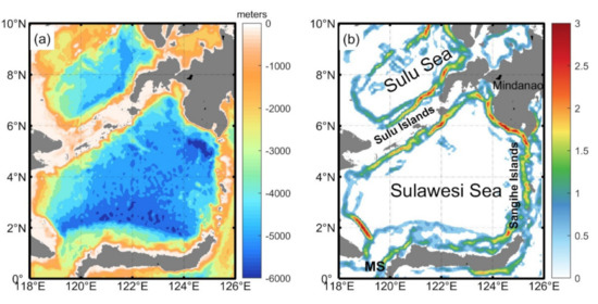
Figure 1.
(a) Bathymetry of the Sulu-Sulawesi Seas. (b) Slope criticality γ/c. (c = [(ω2 − f2)/(N2 − ω2)]1/2), which indicates the internal tide propagation angle to the horizontal, and γ is the bottom gradient.) The study region area is 0° to 10°N, 118° to 126°E near the equator. MS: Makassar Strait. The Sulawesi Sea is semi-closed, connected with the Makassar Strait to the south and the Western Pacific to the east. The Sulu Island chain forms the southern edge of the Sulu Sea and the northern edge of the Sulawesi Sea.
In this paper, to clarify semidiurnal internal tides in the Sulu-Sulawesi Seas, we are motivated to extract the internal tides using a practical plane-wave analysis method [22], which resolves multiwave interference well. From a global view, satellite altimetry shows that the Sulu Island chain radiates the transbasin coherent M2 internal tidal beams [8,29]. However, the multidirectional internal tidal beams are usually represented by the strongest beam in the small-scale basin and become undetected. The decomposition of the multidirectional wave fields allows the covered internal tides to be exposed. Accumulating multiyear satellite altimeter data, multi-satellite altimetry with denser ground tracks can resolve the internal tide with a short wavelength. In Section 2, the satellite altimeter data and plane-wave analysis method will be described. We will propose the semidiurnal internal tide field of the Sulu-Sulawesi Seas in Section 3, with a focus on the interference of multisource internal tides. The interference patterns are explained by a line source model. Section 4 discusses the reflection and energy of internal tides. Section 5 summarizes the results and conclusions.
2. Data and Methods
2.1. Satellite Altimeter Data
In this paper, we used the sea surface height (SSH) observations combined by multiple altimeter satellites, including TOPEX/Poseidon (TP), Jason 1, 2, and 3 (J1, J2, and J3), Geosat Follow-On (GFO), Envisat (EN), and European Remote Sensing Satellite 1 and 2 (ERS-1 and ERS-2). The satellites usually take over and continue the previous satellite missions. Thus, a series of satellites have the same parameters, including the ground track and the repeated cycle (Figure 2a). According to satellite ground tracks, the SSH data are divided into four sets, namely TPJ (TP, J1, J2, and J3), TPT (TP tandem mission), ERS (ERS-1 and ERS-2), and GFO (Figure 2c). Standard corrections for geophysical effects, surface wave bias, and atmospheric effects are applied to process the SSH measurements. Global Ocean Tide 4.7 (GOT4.7) was used to correct the barotropic tide and loading tide. The noise measurement error on the same scale in different satellites is less than the amplitude of internal tides in our survey region. Our study area extends from 118°E, 0° to 126°E, 10°N to contain the Sulu-Sulawesi Seas. To avoid the issues of tide aliasing in marginal seas caused by satellite altimetry measurements, measurements of water depths less than 400 m were eliminated. The reference depth is determined based on the sensitivity analysis of different depths. The setting of a threshold is necessary because the quality of satellite altimeter data in coastal areas is not good enough. The Copernicus Marine and Environment Monitoring Service (CMEMS) is responsible for processing and distributing SSH measurements. The satellite SSH products were downloaded on 16 July 2020. A global mode-1 M2 internal tide field was constructed using a similar dataset [8].
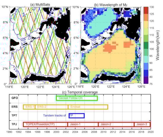
Figure 2.
Satellite altimeter data and wavelength of M2 internal tide. (a) Tracks of multiple satellites (MultiSats). The colors correspond to the boxes in (c). (b) The wavelength of the mode-1 M2 internal tide is calculated from annual-mean ocean stratification in the World Ocean Atlas 2018 (WOA2018). (c) The duration of satellite altimeter observation is from 1993 to 2020.
These datasets have different temporal lengths and spatial coverage. The repeat periods of ERS, GFO, and TPJ are 35, 17, and 10 days. Based on the Rayleigh criterion, the M2 and S2 internal tides can be reliably separated by the long enough datasets. The ground tracks of TPJ (TPT), GFO, and ERS are 254, 488, and 1002. The datasets’ along-track resolution is about 6–7 km, sufficient to resolve internal tides. Noise signals and noise-affected short wavelengths are removed from measurements in the along-track noise filtering with a cutoff wavelength of 65 km. Figure 2b shows the theoretical wavelengths of mode-1 M2 internal tides in the Sulu-Sulawesi Sea, which range from 75 km to 130 km. Because of the distinct stratification caused by the background flow, the wavelengths between the two basins are different. This cutoff wavelength is less than the theoretical minimum wavelength of mode-1 M2 internal tides and denotes the minimum wavelength associated with the dynamical scales to be statistically resolved by the altimetry.
2.2. Two-Dimensional Plane-Wave Fit
Internal tides were extracted by a 2-D plane-wave fit method, using satellite altimeter data with a large spatial coverage. Plane-wave fitting is an extension of traditional point-wise harmonic analysis. This method was first proposed by Ray and subsequently promoted by Zhao [30]. Through plane-wave fitting, the propagation direction and amplitude of the internal tide can be determined by solving multiple stable internal tidal waves in any direction on the plane.
where k0 and ω0 are the tidal frequency and wavenumber, respectively, and x and y are the east and north in the Cartesian coordinates. The expected output, including tidal wave amplitude a, phase ϕ, and propagation direction θ, is obtained by fitting plane waves to satellite SSH data. The buoyancy frequency N, wavenumber k0, and phase velocity Cn are calculated based on WOA2018 [31]. The WOA2018 is a collection of objectively analyzed ocean water quality parameters which has been widely used in ocean models and the corroboration of satellite data.
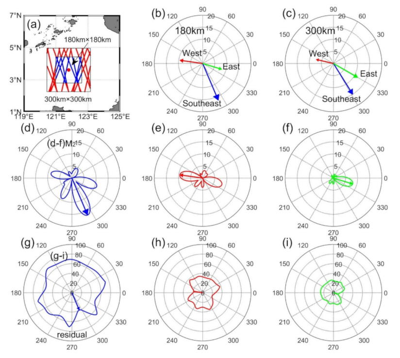
An example is shown in Figure 3 to illustrate the process of extracting mode-1 M2 internal tides. Internal tides are extracted using over 1 × 10⁵ SSH data in a selected window centered at 3.6°N, 121.8°E (Figure 3a). First, using the least-square fitting, the amplitude and phase of a plane-wave are determined in each compass direction with a 1° angular resolution. When we plotted the amplitudes in polar coordinates as a function of direction, the lobes appeared and indicated the internal tidal beams. The amplitude and direction of the first M2 internal tide are determined by the largest lobe (Figure 3d). Then, the phase and direction corresponding to the maximum amplitude is determined. The amplitude maximum corresponds to the residual minimum in the same direction (Figure 3g). When the first internal tide wave is identified, its signal can be reproduced and then removed from the original measurements. The extraction process above is repeated (Figure 3e,f). The residual variance also varies with the direction (Figure 3g–i). The new maximum amplitude tidal wave can then be considered as another tidal wave direction. In this study, five internal tidal waves are extracted in a fitting window of 180 km by 180 km at each grid point, based on a sensitivity analysis of different sizes (Figure 3b,c). The size of the window is about one and a half wavelength of mode-1 M2 internal tides in the Sulu-Sulawesi Seas. The last two internal tide waves are too small, so only the first three waves are presented in Figure 3.

Figure 3.
An example illustrates the plane-wave fit method. (a) A 180-km wide fitting window and a 300-km wide fitting window are centered at 3.6°N, 121.8°E, displaying multi-satellite SSH measurements in this region. (b) Three determined internal tidal waves in a fitting window of 180 km by 180 km. (c) As in (b), but for a fitting window of 300 km by 300 km. (d) Amplitudes (mm) show as a function of direction obtained in the plane-wave fit. The amplitude and direction of the first M2 internal tide are determined by the largest lobe. (e), (f) As in (d), but for westward and eastward waves. After removing the first internal tidal wave from the original measurements, the second M2 internal tidal wave is determined by repeating the procedure. (g) Residual variance (mm2) vs. direction in the plane-wave fit. (h), (i) As in (g), but for westward and eastward waves.
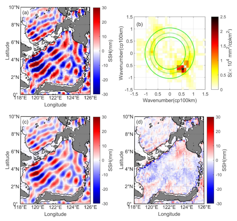
The plane-wave fit method is applied at a regular grid resolution of one-tenth degree (0.1° longitude by 0.1° latitude) in the Sulu-Sulawesi Seas. The five extracted waves get summed in each grid point. Besides, the internal tide solution exists in water deeper than 400 m. Figure 4a presents the map of the mode-1 M2 internal tide field. From the SSH pattern seen in satellite altimetry, the generation sites for the internal tides appear to be the Sulu and Sangihe Island chains, favoring a spatially inhomogeneous SSH field in the Sulu-Sulawesi Seas. An interference pattern means that mooring measurements at different locations vary greatly. Neighboring fitting windows are mostly overlapped, due to the large window and small grid, producing a smooth amplitude, phase, and direction. However, because mesoscale eddies contaminate the internal tide solution in the Sulu-Sulawesi Seas [32,33], some SSH perturbations exist in the internal tide field. A 2-D band-pass filter is required to clean the internal tide field.

Figure 4.
Mapping the M2 internal tide from satellite altimetry. (a) The five-wave superimposed M2 internal tide SSH field was constructed by plane-wave analysis from along-track altimeter measurements. (b) 2-D wavenumber spectrum of (a). The theoretical wavenumber is indicated by the dotted-line circle, and the filter’s cutoff wavenumbers are indicated by the solid-line circles. They are [4/5 8/5] times the theoretical wavenumber. (c) The M2 internal tide SSH field, obtained from the 2-D wavenumber band-pass filtering of (a). (d) Nontidal noise, obtained from the difference between (a,c).
2.3. Two-Dimensional Bandpass Filter
The nontidal noise in the M2 internal tide field is removed by a 2-D band-pass filter (Figure 4). It processes the internal tide field by preserving the internal tides that meet the theoretical wavelengths. Figure 4b shows the two-dimensional wavenumber spectrum conducted by processing the noisy internal tide field on a regular spatial grid. It shows a nearly circular energy pattern indicated by a dotted circle corresponding to a wavenumber of 8 × 10⁻³ cpkm for the mode-1 M2 internal tide. Its reciprocal corresponds to the theoretical wavelength (Figure 2b). Ray and Zaron [29] constructed a global map of modal wavelengths by applying a two-dimensional wavenumber spectrum. The cutoff wavenumbers are indicated by solid circles, which are chosen as [4/5 8/5] times the theoretical wavenumber. Figure 4c shows 2-D band-pass filtered internal tide field with a smooth pattern. Figure 4d gives a residual field representing the nontidal noise acquired from the difference between Figure 4a,c. Because the wavenumber varies more dramatically in small basins, the wavenumber band is broader than the similar band shown by Zhao [22], who fully demonstrated that the 2-D filter does not lead to blind directions. The results will be discussed in Section 3.1.
2.4. Phase Speed and Energy Flux
The horizontal scale of internal tide is much larger than the mean ocean depth. The variable separation method is widely applied to simplify with hydrostatic approximation [34]. A sum of normal vertical modes in a stratified ocean expresses internal tides. We study the first mode of internal tides in this paper. The buoyancy frequency profile N(z) decides the modal structure in the vertical. Φ(z) presents the vertical displacement structure. The following eigenvalue equation determines the modal structure [35]
which satisfies the boundary condition Φ(−H) = Φ(0) = 0, where H is the ocean depth and c is the eigenvalue speed. The buoyancy frequency profiles are calculated from WOA2018.
In a non-rotating fluid, the eigenvalue speed c is the phase speed. Considering the effect of the Earth’s rotation (Ω), the dispersion relation of an internal wave is
where k is the wavenumber, and the inertial frequency is expressed as f ≡ 2Ω sin(latitude). Equation (3) suggests that the internal tide’s wavelength usually increases with latitude, with constant depth and stratification. Before we apply the plane-wave fit method, we will calculate the internal tide’s wavenumber as an input parameter. The phase velocity cp is calculated from c,
where ω stands for the tidal frequencies. Equation (4) also suggests that the internal tide’s phase speed increases with latitude, which causes the refraction of internal tide. Due to a tidal frequency ω > f, phase velocity cp is always greater than c.
Using the vertical modal structures Φ(z), The SSH amplitude can deduce the interior displacement of internal tides. Then, the energy flux of the mode-1 internal tide can be vertically integrated by
where Fn(H, N, ω, f) characterizes the depth-integrated energy flux per unit amplitude of 1 cm at the surface. It is a function of the inertial frequency f, the tidal frequency ω, ocean stratification N(z), and water depth H, and if Fn is determined, the energy flux will be proportional to the amplitude squared. We refer readers to the papers [8,36], which described the calculation procedure in detail.
3. Results
3.1. Decomposed M2 Internal Tides
This study reveals the constructed M2 internal tide field and its three decomposed components in the Sulu-Sulawesi Seas (Figure 5). The black arrows indicate depth-integrated fluxes, which point away from where they are generated. The M2 internal tide field can be separated into three components by the plane-wave fit method due to their different propagation directions (Figure 5b–d). They are southeastward (270–320°), non-dominant directional (−40–50° and 250–270°), and the westward component (90–250°), respectively. We select the internal tides with the maximum amplitude in the chosen directions in each grid point. Unlike Luzon Strait, where multidirectional internal tides propagate away and are observed by satellite altimetry, the Sulu Island chain radiates multidirectional internal tides, which are represented by the biggest internal tide in the small sea basin. Multidirectional decomposition allows the originally covered internal tides to be exposed. The decomposed components have stable phases and wavefronts, compared to the original M2 internal tide field. Multiple waves superpose to form an intricate interference pattern. For example, three tidal beams are marked by green lines and dots (Figure 5a). We refer to the M2 internal tide field simulated by two global numerical models, including GOLD [13] and STORMTIDE [37]. Both models show the existence of the three tidal beams. We will explain the formation of three internal tidal beams in Section 3.3.
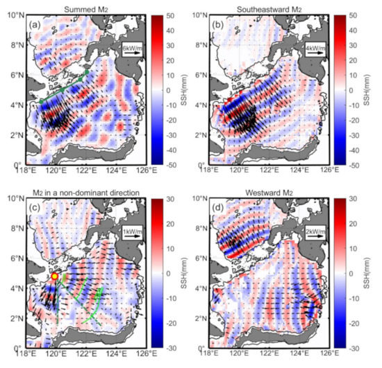
Figure 5.
The M2 internal tide field is decomposed in the Sulu-Sulawesi Seas. Black lines indicate isobathic contours of 400 m. (a) The five-wave-summed M2 internal tide field. Three internal tidal beams are marked by green lines and dots. The internal tide field can be divided into three components. (b) The southeastward component (270–320°). (c) The M2 internal tides in a non-dominant direction consist of the eastward component (−40–50°) and the southward component (250–270°). Two dash green lines indicate a 270° direction and a 320° direction. The yellow dot marks out the Sibutu Passage. The green curves indicate ISWs. (d) The westward component (90–250°). The depth-integrated energy fluxes are shown as black arrows.
The internal tidal wave with the maximum amplitude is separated in the direction (270–320°) on every grid point. Figure 5b displays the southeastward internal tide from the Sulu Island chain. When the internal tide propagates toward the Sulawesi Sea, its isophase lines are almost parallel to the shoreline of the Sulu Island chain. We believe that the feature is formed by the interference of internal tides with similar strength from multiple point sources in the chain. The transbasin internal tide propagates across almost the entire basin with isophase contours, arriving at the Sulawesi continental slope. The fate of the internal tide reaching the continental slope is an open question. We will investigate it in the discussion part.
A group of the M2 internal tides emanate from the Sulu Island chain into the Sulawesi Sea in a non-dominant direction (Figure 5c). They consist of the eastward component (–40–50°) and the southward component (250–270°). The yellow dot indicating the Sibutu passage as a hypothetic point source radiates a cylindrical internal tidal wave with a missing piece. The missing piece is outlined by two dash green lines. The amplitude of the southeastward internal tide is about 40 mm, and the amplitude of a cylindrical internal tidal wave is about 15 mm. The eastward ISWs observed by Liu and D’Sa are spatially coincident with the internal tidal wavefronts (Figure 5c). For the first time, the cylindrical M2 internal tide in the Sulawesi Sea is reported. The recognition of this covered beam benefits from the plane-wave fit method. Here we explain the missing piece of the cylindrical internal tide. The M2 internal tides are separated from the point source and the other source over the Sulu Island chain due to different propagating directions. In contrast, we cannot separate them where their propagation directions become close. The missing piece corresponds to the dominant direction shown in Figure 5b, enhancing the strength of the southeastward internal tide. In addition, the eastward M2 internal tides start from the continental slope in the western Sulu Sea along 119°E ranging from 6 to 9°N (Figure 5c). The weak eastward internal tide propagates along the Sulu Island chain and significantly modulates the dominant northward internal tide from the Sulu Island chain.
Figure 5d shows the westward internal tides from Sulu and Sangihe Island chains. The northwestward internal tides emanate from the Sulu Island chain into the Sulu Sea, propagating in almost the same direction. The internal tide causes a relatively consistent wave and flux pattern in the basin, which agrees well with HYCOM results around the Sulu Sea [38,39]. The Sangihe Island chain is another strong generation source that radiates westward internal tides [40]. The northern and southern sections of the Sangihe Island chain radiate two westward internal tidal beams into the Sulawesi Sea. Two internal tidal beams propagate at an angle and interfere with each other.
3.2. The Dominant Tidal Beam and Internal Solitary Waves
The relation of internal tides and ISWs in the Sulu-Sulawesi Seas is explored by investigating their spatial distribution. The internal tides evolve nonlinearly to generate ISWs from the Sulu Island chain [41,42,43]. Field measurement [44] and satellite observations have confirmed this relation [45]. Figure 6a shows the internal tides superposed with ISWs observed by Liu and D’Sa in 2019 [45]. The relation is revealed by their spatial distribution. The ISWs that are indicated by black curves are spatially coincident with the internal tidal wavefronts (Figure 6a).
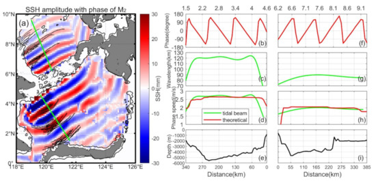
Figure 6.
(a) M2 internal tides and ISWs in Sulu-Sulawesi Seas. Black curves indicate ISWs. The green lines indicate the paths of two M2 beams. (b–i) The M2 internal tides propagate along a definite direction: (b–e) in the Sulawesi Sea and (f–i) in the Sulu Sea. Internal tides phase (Figure 6b,f). Wavelength (Figure 6c,g). Phase speed (Figure 6d,h). The theoretical and observational values are shown as red and green curves, respectively. Submarine topography (Figure 6e,i).
Liu and D’Sa [45] reported that ISWs are observed to propagate into the Sulu Sea and the Sulawesi Sea, showing the behavior of a spring-neap tidal cycle. The ISWs in the Sulawesi Sea are less frequently observed compared to those in the Sulu Sea. Zhang et al. [43] further confirmed that ISWs are mainly observed in the shallower western zones rather than the deeper eastern areas in the Sulu Sea. Tessler et al. [42] estimated the observed energy of the waves, maintaining baroclinic tidal mixing rates. A large number of ISWs accompany the internal tides, which indicates that their common generation source is the Sulu Island chain.
The green lines suggest the propagation paths of two M2 beams in the Sulu- Sulawesi Seas. The along-beam phase speed of M2 internal tide is examined by comparing the theoretical and altimetric results. Many factors affect the phase speed, including the depth and latitude. We calculated these factors along the two green lines, and the calculation procedure is illustrated in Figure 6b–i. First, the along-beam phase usually increases with the propagation distance in the Sulu-Sulawesi Sea, respectively (Figure 6b,f). Then, the polynomial fitting is employed to smooth the along-beam phase. The wavelength is calculated from the relation of phase gradient to distance (Figure 6c,g). The graphs show that the wavelength is mainly affected by the basin’s depth rather than the Coriolis parameter near the equator. Finally, the phase speed is deduced from the relation of frequency and wavelength (Figure 6d,h). For comparison, light green curves indicate the theoretical phase speeds extracted from WOA2018 [31]. Due to the rapid decrease in the depth of submarine topography, the low values of the theoretical phase speed appear at starting and ending points (Figure 6e,i); meanwhile, the satellite-derived phase speeds coincide with the theoretical phase speeds.
3.3. Sulu Sea vs. Sulawesi Sea
Semidiurnal internal tides display an apparent contrast between the Sulu Sea and the Sulawesi Sea. The Sulu Island chain radiates the semidiurnal internal tides northward into the Sulu Sea and southward into the Sulawesi Sea. The amplitude of the northward M2 internal tide is about 20 mm, about half of the southward one. The northward internal tide from the Sulu Island chain propagates in almost the same direction. However, multidirectional internal tides from the Sulu Island chain are superposed on the westward internal tide emanating from the Sangihe Island chain, forming a complex interference pattern in the Sulawesi Sea. The wavelength of the internal tide in the Sulawesi Sea is longer than that in the Sulu Sea. In summary, internal tides in the Sulu Sea and the Sulawesi Sea have different strengths, directions, and wavelengths. The reason for this contrast is that the number and distribution of their generation sources are distinct. Thus, the internal tides in the Sulawesi Sea have significant spatial inhomogeneity due to multisource interference. Next, we will further investigate the distinctions of internal tides between the two basins in detail from their multiple generation sources and multiwave interference process.
3.3.1. Comparison of Multiple Generation Sources
The multidirectional internal tides emanate away from two island chains, suggesting the presence of multiple sources in the boundaries. The phenomenon captured by the satellite altimeter is clarified in this section. Previous studies have investigated the barotropic tide in the Sulu-Sulawesi Seas by mooring measurements, satellite altimetry, and numerical models [46]. The model product is generated by a TPXO developed by Egbert and Erofeeva [26]. Figure 7a shows M2 barotropic tidal ellipses and volume transport in the Sulu-Sulawesi Seas. The M2 tide enters the Sulawesi Sea via the Sulu Island chain (Figure 7b). Strong tidal currents mainly occur in the eastern section of the Sibutu Passage in the Sulu Island chain, corresponding to the hypothetic point source. Affected by the rugged terrain, the tidal currents follow multiple directions, favoring a multidirectional internal tide generation. In contrast, the tidal currents mainly flow across the Sangihe Island chain (Figure 7c). The southern section of the Sangihe Island chain is the main channel of volume transport.
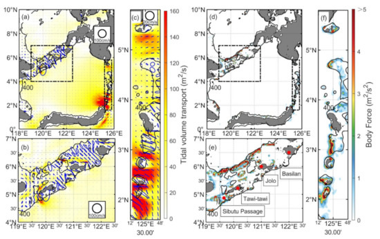
Figure 7.
M2 barotropic tide from TPXO and body force. Isobathic contours of 400 m are shown as black lines. (a) M2 barotropic tidal ellipses and volume transport. Tidal ellipses are shown in blue. Two dotted boxes indicate two island chains. (b,c) are partial enlargements of (a). (b) Tidal ellipses and volume transport in the Sulu Islands chain. (c) As in (b), but in the Sangihe Islands chain. (d) Barotropic tidal body force. (e,f) are also partial enlargements of (d). (e) Barotropic tidal body force in the Sulu Islands chain. The four red dots represent Basilan Island, Jolo Island, Tawi-tawi Island, and Sibutu Passage. (f) As in (e), but in the Sangihe Islands chain. The dark red in the colorbar indicates values greater than five.
The barotropic tidal body force is used to reveal generation sites. The calculation of the barotropic tidal body force is expressed as
where H presents the basin depth, ∇H is the bottom gradient, Q is the barotropic tidal volume transport from TPXO, ω is the M2 tidal frequency, and N2 is the buoyancy frequency calculated from stratification from WOA2018. Figure 7d shows the barotropic tidal body force in the Sulu-Sulawesi Seas. In particular, Sibutu Passage, near Tawi-tawi Island, and Jolo Island, along the Sulu Island chain, are strong sources (Figure 7e). The body force shows that the generation sites are on the northern and southern sections of the Sangihe Island chain (Figure 7f). It reveals that strong conversion sites are scattered around the two island chains, which is consistent with previous work [43].
3.3.2. Comparison of Multiwave Interference Process
The decomposed internal tidal waves are revealed by the satellite altimeter observation. Their interference mechanism should be taken into account to interpret the complex structures of the SSH pattern. To illustrate the SSH pattern observed by satellites, an ideal line source model is employed to simulate the interference between multidirectional internal tidal waves. The line source model was proposed by St. Laurent et al. [47] and subsequently promoted by Rainville et al. [7]. The model uses a zero-width ridge as the source and a sinusoidal barotropic tidal current perpendicular to the ridge. Rainville et al. [7] noted that the simple model could describe the surface elevations caused by baroclinic tides:
where ζ0, r0, β, a0 are the wave amplitude, the source radius, the attenuation coefficient, and the “arc length”. ω, kr, and ϕ0 are respectively the M2 frequency, wavenumber, and phase. The internal tidal wave is limited to the distance within r > r0 and the direction between θ0 ± (a0/2r0). The altimetric results determine the parameters applied in the line source model (Table 1). The line source model clarifies the formation of interference by characterizing the plane waves. The phase Φ0 of the internal tides is associated with the phase of the barotropic tides at the generation sites [47]. The wavelength for mode-1 M2 internal tides is obtained by averaging the theoretical wavelength from WOA2018.

Table 1.
Parameters are used to reproduce the interference in the Line Source Model.
Internal tide generation sites along the two island chains are not uniform. The line source model described a wave propagation that can have various levels of source numbers. For example, a few sources at the major generation sites can be superposed to create a line source, and larger amounts of sources along island chains also create a line source with a similar spatial pattern. Here we retain only the six dominant sources in the line source model (Figure 8). Figure 8a shows that a line source is used to characterize the smooth internal tide. Figure 8b shows the Sibutu Passage as a point source. The superposition of a line source and a point source presents spatial variability and three strong beams (Figure 8c). The northern and southern sections of Sangihe Island chain as two sources are shown in Figure 8d,e. Figure 8f shows the interference of M2 internal tides from the two sources. The interference between M2 internal tides from the continental slope in the eastern Sulu Sea and Sulu Island chain is not shown here. Based on the superpose principle, due to the destructive effects of interference, the SSH becomes weak between the beams. Internal tidal waves form nodes and antinodes not only in the SSH field but also in the energy flux.
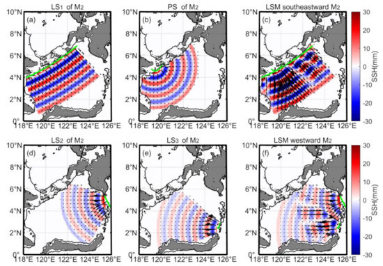
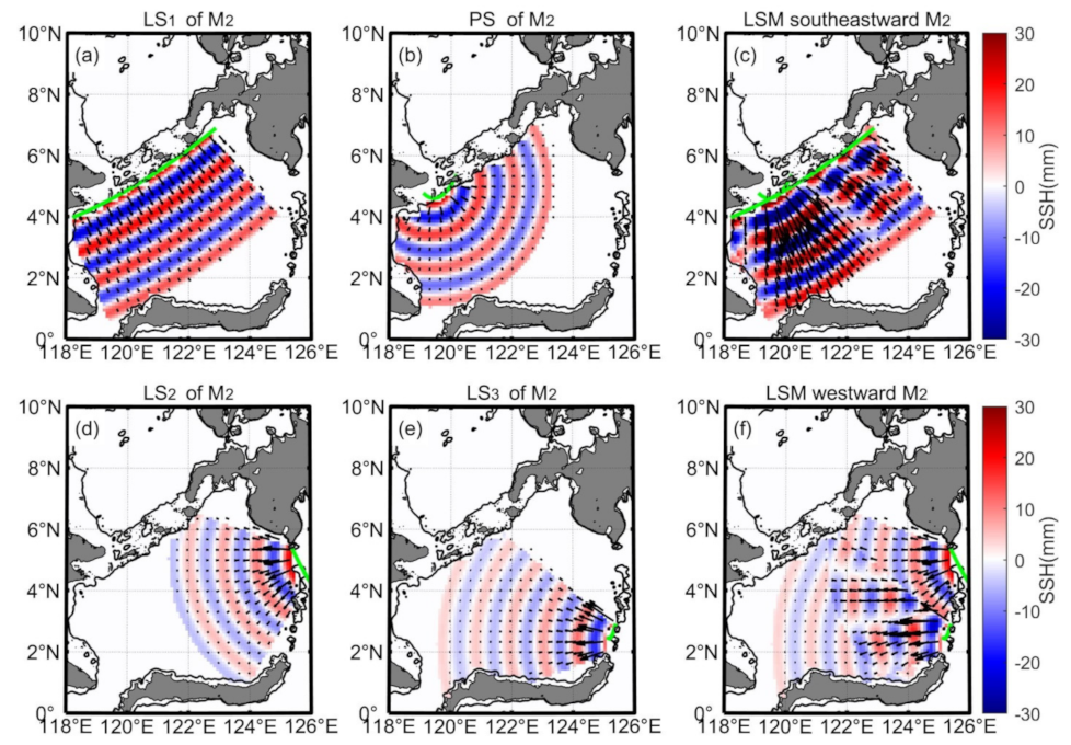
Figure 8.
The line sources in the ideal line source model. (a) A line source along the Sulu Island chain. (b) A point source is located on the Sibutu Passage. (c) Interference pattern in the Sulawesi Sea superimposed to (a,b). The line source is located on (d) the northern section and (e) the southern section of the Sangihe Island chain. (f) Interference pattern in the Sulawesi Sea superimposed to (d,e). Parameters of LSM are listed in Table 1.
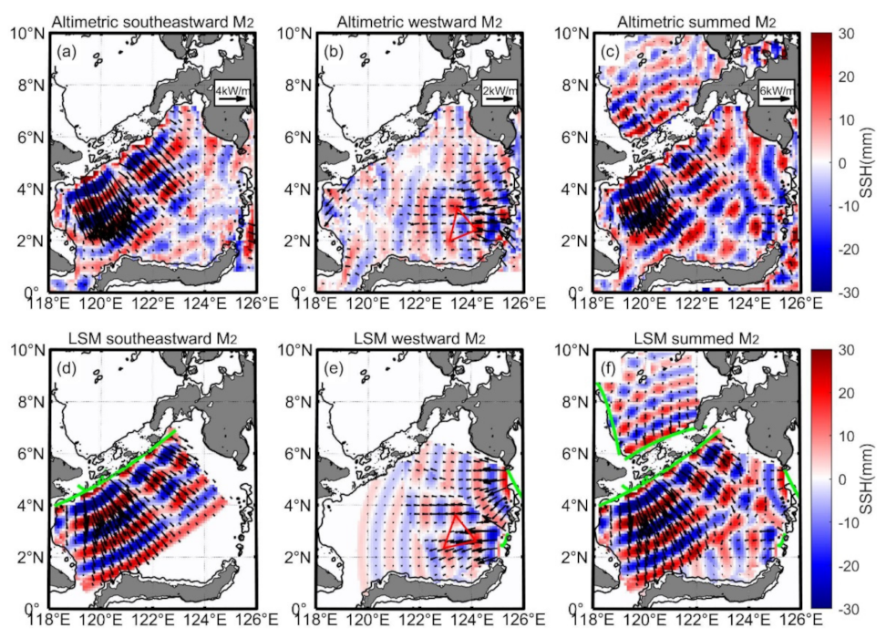
The interference pattern caused by several sources in the LSM explains the complex structures of baroclinic SSH observed by satellite altimetry. Interference patterns in the Sulu-Sulawesi Sea are present by the line source model and satellite altimetry (Figure 9). Different from the decomposed internal tidal fields in Figure 5, the internal tides observed in each grid point get summed in the chosen direction (Figure 9a–c). To demonstrate the spatial pattern of the M2 internal tide field modulated by multiwave interference, the Sulawesi Sea is divided into two fields. The first field in the western basin is predominantly influenced by internal tides from the Sulu Island chain. The second field in the eastern basin is influenced by internal tides from the Sangihe Island chain. Two island chains as the boundary of the Sulawesi Sea radiate internal tides, contributing to the interference pattern. Finally, internal tides from both island chains superposed together to construct the spatial pattern in the Sulu-Sulawesi Sea.
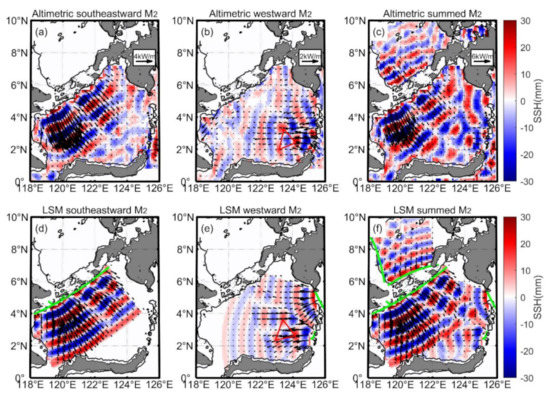
Figure 9.
Interference patterns in the Sulawesi Sea by satellite altimetry and the line source model. (a) Altimetric M2 internal tide from the Sulu Island chain. (b,c) as in (a), for the M2 internal tide from the Sangihe Island chain and both island chains. (d) M2 internal tide from the Sulu Island chain in the ideal line source model. (e,f) as in (d), for the M2 internal tide from the Sangihe Island chain and both island chains. The red triangle represents the enhancement area. The green curves indicate generation sources.
In the western basin of the Sulawesi Sea, a cylindrical internal tidal wave from the Sibutu Passage significantly modulates the dominant internal tides from the Sulu Island chain. The interference shapes three internal tidal beams with elevated energy flux magnitude (Figure 9a). The three internal tidal beams with various strengths are all presented by satellite altimetric observation and the ideal line source model (Figure 9a,d). This interference pattern has been suggested by global satellite observations [8]. This feature is similar to that at the Hawaiian Ridge, where internal tides interfere to form distinct beams [7]. We can conclude that the weak internal tide modulates the SSH field, contributing to the inhomogeneous distribution of M2 internal tides. In the eastern basin of the Sulawesi Sea, the internal tides are generated at the northern and southern sections of the Sangihe Island chain. One can see that an enhanced central internal tidal beam is formed at the intersection of their propagation paths (Figure 9b,e). In the whole sea basin, the complex SSH pattern from the idea line source model is consistent with the satellite altimetric observation. The internal tide in the Sulu Sea propagates about four wavelengths (Figure 9f), while the internal tide in the Sulawesi Sea propagates about three wavelengths for approximate distance. Eventually, the sources are summed to be compared to the SSH for satellite altimetric observations (Figure 9c). A spatially inhomogeneous SSH field is shaped by internal tides from the Sulu and Sangihe Island chains. Semidiurnal internal tides display complex and distinct geographical variations between the Sulu and Sulawesi Seas. Many simplifications are made in the line source model, including tidal beams perpendicular to the source ridge, coherent and two-dimensional [47]. Furthermore, the line source model neglects the topography-scattering effects to characterize the interference of plane waves ideally. An ideal line source model applied in the small basin should take into account neighboring sources and the short propagation distance.
3.4. S2 Internal Tides
The S2 internal tide field in the Sulu-Sulawesi Seas is constructed by fitting plane waves (Figure 10a). The specific frequency and wavelength of the S2 internal tide are input parameters in the extraction process. Like point harmonic analysis, plane-wave analysis can extract multi-frequency internal tide signals in one step. The wavenumber band of the 2-D band-pass filter processing the S2 internal tide field is similar to that of the M2 internal tide. Because of tidal aliasing, the S2 tidal signals could not be extracted from ERS satellite altimeter data which are excluded in the extraction process. Although the amount of data is reduced, the same fitting window as that of the M2 internal tide is still used after different window size attempts to investigate the spatial propagation characteristics of the S2 internal tide.
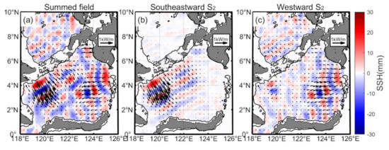
Figure 10.
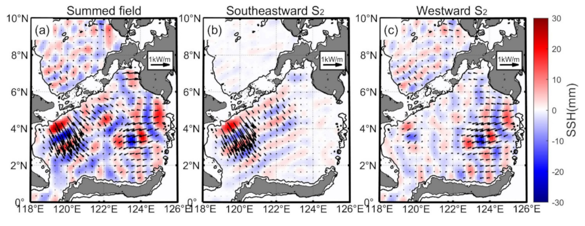
The mode-1 S2 internal tide field is decomposed. (a) The five-wave-summed S2 internal tide field. The internal tide field can be divided into two components. (b) The southward component (250–330°). (c) The westward component (90–270°). The S2 internal tidal energy fluxes are shown as black arrows in (a–c). Isobathic contours of 400 m are indicated as black lines, respectively.
Figure 10a shows the superposition map of mode-1 S2 internal tides. Consistent with the M2 internal tide field, the Sulu and Sangihe Island chains are also essential generation sources for the S2 internal tides. Several internal tidal beams are shaped by multiwave interference. Then, we separated the southward and westward components, respectively. Figure 10b shows the S2 internal tidal beams propagated from the Sulu Island chain into the Sulawesi Sea. They propagate about three wavelengths and become undetected by satellite altimeters. The western internal beam is stronger than the eastern one, which indicates that the Sibutu Passage is also an energetic generation site. The SSH ratio of S2 to M2 is 0.46, consistent with their ratio in the global ocean [48]. However, differently from M2 internal tides, we find the lack of a stable and continuous eastward S2 internal tide signal. We deduce that the eastward S2 internal tide is very weak and becomes undetectable.
Westward S2 internal tides emanate from the Sulu and Sangihe Island chains (Figure 10c). On the one hand, two internal tidal beams propagate from the Sangihe Island chain. They interfere with each other and enhance the S2 internal tidal amplitude and energy flux. The westward S2 beams travel a shorter distance than the M2 beams because nontidal noise disturbs the weak S2 internal tide more easily. On the other hand, the northward internal tidal beam emanates from the Sulu Island chain into the Sulu Sea. The internal tide passes through the basin and reaches the other side due to the stable ocean environment.
4. Discussion
4.1. Reflection on the Sulawesi Continental Slope
In this section, we investigate the fate of the transbasin M2 internal tide in the Sulawesi Sea (Figure 11a). Theoretically, a small fraction of the M2 internal tide is expected to reflect into the Sulawesi sea, since the Sulawesi slope is supercritical to M2 (Figure 1b). The incident and reflected M2 internal tides have been investigated in marginal seas by satellite altimeters, such as the Tasman Sea [49]. The incident and reflected internal tides can be separated according to their propagation directions. This separation is attributed to the multiwave internal tidal field decomposed by the plane-wave fitting method (Figure 3). Here, we choose waves in the direction of 280°–330° as the incident internal tides and 0°–70° as the reflected internal tides (Figure 11).
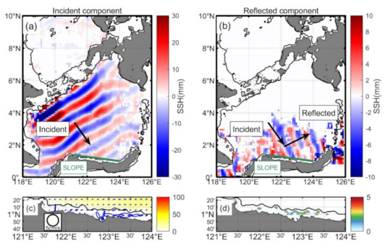
Figure 11.
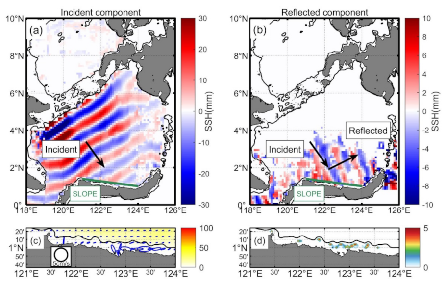
The M2 internal tide reflects in the Sulawesi Sea. (a) Incident part (ranging 280–330°). (b) Reflected part (ranging 0–70°). The Sulawesi slope is denoted as the green line. The incident and reflected waves are shown as two black arrows, respectively. The ratio of the incident and reflected SSH amplitudes near the Sulawesi slope presents reflectivity. (c) M2 barotropic tide ellipse and volume transport in the Sulawesi slope. (d) Barotropic tidal body force in the Sulawesi slope.
Figure 11 shows that the dominant M2 internal tidal beam hits the Sulawesi slope and reflects into the Sulawesi Sea. Snell’s law is used to examine the incident and reflected waves. The black arrow with a 300° incidence angle denotes the incident internal tidal wave. A black arrow toward 28° denotes the reflected wave. The green line denotes the continental slope as the wall. Satellite altimetric observation agrees well with the law of reflection, indicating that the northeastward tidal beam is reflected from the Sulawesi slope. When the dominant internal tidal beam reaches the slope, the amplitude of the incident part is about 6 mm. The amplitude of the reflected wave is about 4 mm. The energy flux is approximately proportional to the SSH squared in Equation (5). Thus, the reflectivity from the incident and reflected energy flux is about 45%. Our estimation may be affected by many factors.
In addition, we need to verify that the northeastward internal tide is not locally generated. We check the tidal ellipses, volume transport, and barotropic tidal body force on the Sulawesi slope. The direction of the tidal current is not consistent with the propagation direction of the reflected internal tide. Therefore, it can be concluded that the northeastward internal tide is formed by reflection rather than local generation. A key point of this paper is to note the existence of the reflection phenomenon but not to estimate the reflectivity accurately. A quantitative estimation of reflectivity requires further field observations and numerical models with a suitable method in the Sulawesi Sea [50].
4.2. Internal Tide Energetics
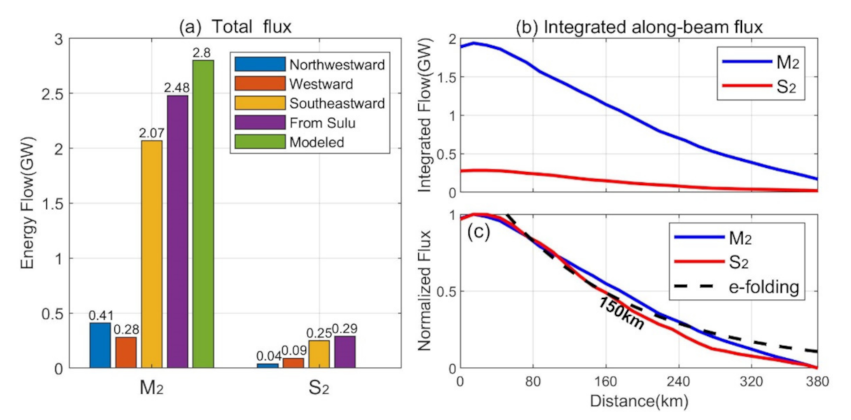
In this section, we estimate the semidiurnal internal tidal energy fluxes from two island chains. The total energy fluxes are integrated along a section across the whole sea basin parallel to the two island chains. For the southeastward M2 internal tide from the Sulu Island chain, we acquire a total energy flux of 2.07 GW. Similarly, we estimate the northwestward energy flux from the Sulu Island chain and westward energy flux from the Sangihe Island chain. The total energy fluxes for the northwestward and westward internal tides are 0.41 and 0.28 GW, respectively. Thus, the total M2 tidal energy flux from the Sulu Island chain is 2.48 GW (Figure 12a). It is about 80% of 2.8 GW from the numerical simulation by Nagai and Hibiya [27]. The westward internal tide is smaller than the model result because only the energy flux in the Sulawesi Sea is considered [51]. Likewise, the energy flux for each direction of the S2 internal tides is estimated. The energy fluxes for the northwestward, westward, and southeastward internal tides are 0.04, 0.09, and 0.25 GW, respectively. The total semidiurnal tidal energy fluxes from the Sulu and Sangihe Island chains into the Sulawesi Sea are about 2.7 GW, measured by satellite altimetry.
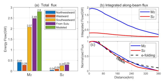
Figure 12.
The total energy fluxes and the decay rate of the southeastward internal tide. (a) The total internal tidal energy flux from two island chains. (b) The decay of the southeastward internal tide. (c) Internal tides energy flux after normalization. The E-folding scale of 150 km is indicated as the dashed curve.
Furthermore, we estimate the decay rate of the dominant internal tide (Figure 5b). We sample the internal tide from the Sulu Island chain to the Sulawesi slope using 30 equidistant sections. We integrate them along each section, which is perpendicular to the energy fluxes. The blue line and red line in Figure 12b respectively denote the M2, and S2 energy flux obtained using plane-wave fitting. Figure 12c indicates the M2 and S2 internal tides energy flux after normalization. Even though their amplitudes are different, both of them decay at close rates. The E-folding decay scale of 150 km is indicated as the dashed curve. The short e-folding scale may be the result of either undetectable incoherent internal tides or real dissipation.
5. Conclusions
In this paper, we apply the plane-wave analysis method to construct the regional semidiurnal internal tidal field in the Sulu-Sulawesi Seas from multi-satellite altimeter data. We separately decompose the internal tidal field due to different propagation directions. The components obtained from the decomposition contribute to a better understanding of the formation and propagation of internal tidal beams. The multidirectional internal tides and their interference are revealed in the Sulu-Sulawesi Seas. We presented the geographic distribution of the semidiurnal internal tidal beams from the Sulu and Sangihe Island chains. The internal tides in the Sulawesi Sea dissipate in the semi-closed basin, causing strong tidal mixing.
Our main scientific findings are as follows. (1) The constructed M2 internal tidal field is decomposed into three components, which have different propagation directions. The interference pattern is well reproduced by the line source model. (2) The Sibutu passage in the Sulu Island chain acts as a point source that radiates a cylindrical internal tidal wave. (3) The ISWs spatially correspond to the internal tidal wavefronts. The phase speed derived from the satellite is in good agreement with the theoretical phase speed. The above two results confirm that the analysis method can be applied to local small sea basins. (4) The northward M2 tidal energy flux from the Sulu Island chain is 0.41 GW, about 20% of the southward energy flux. The total energy fluxes from satellite altimeters are about 80% of those from numerical simulations in the Sulu Island chain. (5) The M2 and S2 internal tides have a similar decay rate, although the SSH ratio of S2 to M2 is 0.45. (6) The total semidiurnal tidal energy fluxes from the Sulu and Sangihe Island chains into the Sulawesi Sea are about 2.7 GW. It is important to note that these values are all at the lower limits because they are multi-year coherent results. The plane-wave analysis only extracts the temporally coherent internal tide. The internal tides become incoherent due to the variation of the ocean environment, such as mesoscale eddies and circulation [52].
The present study focuses on the coherent internal tides over 20 years. However, recent studies revealed that the internal tides show the spatial distribution and strong seasonal variation in the Indonesian Archipelago and adjacent seas [53,54,55]. In addition, the Sulawesi Sea is the main channel of ITF, which affects the generation and propagation of internal tides. The propagation direction of internal tides from the Sulu Island chain is almost perpendicular to the direction of ITF in the Sulawesi Sea. In contrast, the internal tides propagate from the Sangihe Island chain in the same direction as the ITF, weakening the westward internal tides observed by satellite altimetry. The Sulu-Sulawesi Seas are also identified to be the source of the energetic generation of diurnal internal tides. The investigation of these tides using multi-satellite altimeter is underway.
Author Contributions
Conceptualization, X.Z., Z.X. and Q.L.; methodology, X.Z. and Z.X.; software, X.Z.; writing—original draft preparation, X.Z.; writing—review and editing, Z.X., M.F., Q.L., P.Z., J.Y., S.G., B.Y. and X.Z. All authors have read and agreed to the published version of the manuscript.
Funding
This study was supported by the Strategic Pioneering Research Program of CAS, the National Natural Science Foundation of China, the National Key Research and Development Program of China (XDB42000000, XDA22050202, 92058202, 91858103, 2017YFA0604102, 2016YFC1401404), the CAS Key Research Program of Frontier Sciences, the Key Deployment Project of Centre for Ocean Mega-Research of Science, and the project jointly funded by the CAS and CSIRO (QYZDB-SSW-DQC024, COMS2020Q07, 133244KYSB20190031).
Institutional Review Board Statement
Not applicable.
Informed Consent Statement
Not applicable.
Data Availability Statement
The datasets presented in this study are publicly available. The altimetric sea surface height measurements are produced by Archiving, Validation, and Interpolation of Satellite Oceanographic Data (AVISO) and distributed by the Copernicus Marine and Environment Monitoring Service (CMEMS) via https://marine.copernicus.eu/, (accessed on 25 June 2021). The World Ocean Atlas 2018 is produced and made available by NOAA National Centers for Environmental Information via https://accession.nodc.noaa.gov/NCEI-WOA18, (accessed on 25 June 2021). The TPXO tide model is from the Oregon State University via https://www.tpxo.net/global/tpxo9-atlas, (accessed on 25 June 2021). The internal tide products presented in this paper are available upon request.
Acknowledgments
We would like to thank the editors and three anonymous reviewers whose constructive comments have significantly improved the manuscript.
Conflicts of Interest
The authors declare no conflict of interest. The funders had no role in the design of the study; in the collection, analyses, or interpretation of data; in the writing of the manuscript, or in the decision to publish the results.
References
- Munk, W.; Wunsch, C. Abyssal recipes II: Energetics of tidal and wind mixing. Deep Sea Res. Part I Oceanogr. Res. Pap. 1998, 45, 1977–2010. [Google Scholar] [CrossRef]
- Alford, M.H. Redistribution of energy available for ocean mixing by long-range propagation of internal waves. Nature 2003, 423, 156–162. [Google Scholar] [CrossRef] [PubMed]
- Neale, R.; Slingo, J. The Maritime Continent and Its Role in the Global Climate: A GCM Study. J. Clim. 2003, 16, 834–848. [Google Scholar] [CrossRef]
- Alford, M.H.; Zhao, Z. Global Patterns of Low-Mode Internal-Wave Propagation. Part I: Energy and Energy Flux. J. Phys. Oceanogr. 2007, 37, 1829–1848. [Google Scholar] [CrossRef]
- Egbert, G.D.; Ray, R.D. Semi-diurnal and diurnal tidal dissipation from TOPEX/Poseidon altimetry. Geophys. Res. Lett. 2003, 30, 1907. [Google Scholar] [CrossRef]
- MacKinnon, J.A.; Alford, M.H.; Ansong, J.K.; Arbic, B.K.; Barna, A.; Briegleb, B.P.; Bryan, F.O.; Buijsman, M.C.; Chassignet, E.P.; Danabasoglu, G.; et al. Climate Process Team on Internal Wave-Driven Ocean Mixing. Bull. Am. Meteorol. Soc. 2017, 98, 2429–2454. [Google Scholar] [CrossRef] [Green Version]
- Rainville, L.; Johnston, T.M.S.; Carter, G.S.; Merrifield, M.A.; Pinkel, R.; Worcester, P.F.; Dushaw, B.D. Interference Pattern and Propagation of the M2 Internal Tide South of the Hawaiian Ridge. J. Phys. Oceanogr. 2010, 40, 311–325. [Google Scholar] [CrossRef]
- Zhao, Z.; Alford, M.H.; Girton, J.B.; Rainville, L.; Simmons, H.L. Global Observations of Open-Ocean Mode-1 M2 Internal Tides. J. Phys. Oceanogr. 2016, 46, 1657–1684. [Google Scholar] [CrossRef]
- Chang, H.; Xu, Z.; Yin, B.; Hou, Y.; Liu, Y.; Li, D.; Wang, Y.; Cao, S.; Liu, A.K. Generation and Propagation of M2 Internal Tides Modulated by the Kuroshio Northeast of Taiwan. J. Geophys. Res. Ocean. 2019, 124, 2728–2749. [Google Scholar] [CrossRef]
- Wang, Y.; Xu, Z.; Yin, B.; Hou, Y.; Chang, H. Long-Range Radiation and Interference Pattern of Multisource M2 Internal Tides in the Philippine Sea. J. Geophys. Res. Ocean. 2018, 123, 5091–5112. [Google Scholar] [CrossRef] [Green Version]
- Xu, Z.; Liu, K.; Yin, B.; Zhao, Z.; Wang, Y.; Li, Q. Long-range propagation and associated variability of internal tides in the South China Sea. J. Geophys. Res. Ocean. 2016, 121, 8268–8286. [Google Scholar] [CrossRef]
- Zhao, C.; Xu, Z.; Robertson, R.; Li, Q.; Wang, Y.; Yin, B. The Three-Dimensional Internal Tide Radiation and Dissipation in the Mariana Arc-Trench System. J. Geophys. Res. Ocean. 2021, 126. [Google Scholar] [CrossRef]
- Simmons, H.L.; Hallberg, R.W.; Arbic, B.K. Internal wave generation in a global baroclinic tide model. Deep Sea Res. Part II Top. Stud. Oceanogr. 2004, 51, 3043–3068. [Google Scholar] [CrossRef]
- Robertson, R. Interactions between tides and other frequencies in the Indonesian seas. Ocean Dyn. 2011, 61, 69–88. [Google Scholar] [CrossRef]
- Robertson, R.; Ffield, A. Baroclinic tides in the Indonesian seas: Tidal fields and comparisons to observations. J. Geophys. Res. 2008, 113, C07031. [Google Scholar] [CrossRef] [Green Version]
- Koch-Larrouy, A.; Lengaigne, M.; Terray, P.; Madec, G.; Masson, S. Tidal mixing in the Indonesian Seas and its effect on the tropical climate system. Clim. Dyn. 2010, 34, 891–904. [Google Scholar] [CrossRef]
- Ffield, A.; Gordon, A.L. Tidal Mixing Signatures in the Indonesian Seas. J. Phys. Oceanogr. 1996, 26, 1924–1937. [Google Scholar] [CrossRef] [Green Version]
- Hatayama, T.; Awaji, T.; Akitomo, K. Tidal currents in the Indonesian Seas and their effect on transport and mixing. J. Geophys. Res. Ocean. 1996, 101, 12353–12373. [Google Scholar] [CrossRef]
- Ray, R.D.; Mitchum, G.T. Surface manifestation of internal tides in the deep ocean: Observations from altimetry and island gauges. Prog. Oceanogr. 1997, 40, 135–162. [Google Scholar] [CrossRef]
- Tian, J.; Zhou, L.; Zhang, X.; Liang, X.; Zheng, Q.; Zhao, W. Estimates of M2 internal tide energy fluxes along the margin of Northwestern Pacific using TOPEX/POSEIDON altimeter data. Geophys. Res. Lett. 2003, 30, 17. [Google Scholar] [CrossRef]
- Zaron, E.D. Baroclinic Tidal Sea Level from Exact-Repeat Mission Altimetry. J. Phys. Oceanogr. 2019, 49, 193–210. [Google Scholar] [CrossRef]
- Zhao, Z. Mapping Internal Tides from Satellite Altimetry without Blind Directions. J. Geophys. Res. Ocean. 2019, 124, 8605–8625. [Google Scholar] [CrossRef]
- Jithin, A.K.; Subeesh, M.P.; Francis, P.A.; Ramakrishna, S. Intensification of tidally generated internal waves in the north-central Bay of Bengal. Sci. Rep. 2020, 10, 6059. [Google Scholar] [CrossRef] [PubMed] [Green Version]
- Zhao, Z. Southward Internal Tides in the Northeastern South China Sea. J. Geophys. Res. Ocean. 2020, 125. [Google Scholar] [CrossRef]
- Koch-Larrouy, A.; Madec, G.; Bouruet-Aubertot, P.; Gerkema, T.; Bessières, L.; Molcard, R. On the transformation of Pacific Water into Indonesian Throughflow Water by internal tidal mixing. Geophys. Res. Lett. 2007, 34. [Google Scholar] [CrossRef] [Green Version]
- Egbert, G.D.; Erofeeva, S.Y. Efficient Inverse Modeling of Barotropic Ocean Tides. J. Atmos. Ocean. Technol. 2002, 19, 183–204. [Google Scholar] [CrossRef] [Green Version]
- Nagai, T.; Hibiya, T. Internal tides and associated vertical mixing in the Indonesian Archipelago. J. Geophys. Res. Ocean. 2015, 120, 3373–3390. [Google Scholar] [CrossRef]
- Buijsman, M.C.; Arbic, B.K.; Richman, J.G.; Shriver, J.F.; Wallcraft, A.J.; Zamudio, L. Semidiurnal internal tide incoherence in the equatorial Pacific. J. Geophys. Res. Ocean. 2017, 122, 5286–5305. [Google Scholar] [CrossRef]
- Ray, R.D.; Zaron, E.D. M2 Internal Tides and Their Observed Wavenumber Spectra from Satellite Altimetry. J. Phys. Oceanogr. 2016, 46, 3–22. [Google Scholar] [CrossRef]
- Ray, R.D.; Cartwright, D.E. Estimates of internal tide energy fluxes from Topex/Poseidon Altimetry: Central North Pacific. Geophys. Res. Lett. 2001, 28, 1259–1262. [Google Scholar] [CrossRef] [Green Version]
- Locarnini, R.A.; Mishonov, A.V.; Baranova, O.K.; Boyer, T.P.; Locarnini, R.A. World Ocean Atlas 2018, Volume 1: Temperature; NOAA Atlas NESDIS: Silver Spring, MD, USA, 2019. [Google Scholar]
- Hao, Z.; Xu, Z.; Feng, M.; Li, Q.; Yin, B. Spatiotemporal Variability of Mesoscale Eddies in the Indonesian Seas. Remote Sens. 2021, 13, 1017. [Google Scholar] [CrossRef]
- He, Y.; Feng, M.; Xie, J.; Liu, J.; Chen, Z.; Xu, J.; Fang, W.; Cai, S. Spatiotemporal Variations of Mesoscale Eddies in the Sulu Sea. J. Geophys. Res. Ocean. 2017, 122, 7867–7879. [Google Scholar] [CrossRef]
- Wunsch, C. Internal tides in the ocean. Rev. Geophys. 1975, 13, 167–182. [Google Scholar] [CrossRef]
- Gill, A. Atmosphere-Ocean Dynamics; Academic Press: Cambridge, MA, USA, 1982. [Google Scholar]
- Zhao, Z.; Alford, M.H. New Altimetric Estimates of Mode-1 M2 Internal Tides in the Central North Pacific Ocean. J. Phys. Oceanogr. 2009, 39, 1669–1684. [Google Scholar] [CrossRef]
- Muller, M. On the space- and time-dependence of barotropic-to-baroclinic tidal energy conversion. Ocean Model. 2013, 72, 242–252. [Google Scholar] [CrossRef]
- Hurlburt, H.; Metzger, J.; Sprintall, J.; Riedlinger, S.; Arnone, R.; Shinoda, T.; Xu, X. Circulation in the Philippine Archipelago Simulated by 1/12° and 1/25° Global HYCOM and EAS NCOM. Oceanography 2011, 24, 28–47. [Google Scholar] [CrossRef]
- Metzger, E.J.; Hurlburt, H.E.; Xu, X.; Shriver, J.F.; Gordon, A.L.; Sprintall, J.; Susanto, R.D.; van Aken, H.M. Simulated and observed circulation in the Indonesian Seas: 1/12° global HYCOM and the INSTANT observations. Dyn. Atmos. Ocean. 2010, 50, 275–300. [Google Scholar] [CrossRef]
- Nugroho, D.; Koch-Larrouy, A.; Gaspar, P.; Lyard, F.; Reffray, G.; Tranchant, B. Modelling explicit tides in the Indonesian seas: An important process for surface sea water properties. Mar. Pollut. Bull. 2018, 131, 7–18. [Google Scholar] [CrossRef]
- Chen, G.-Y.; Su, F.-C.; Wang, C.-M.; Liu, C.-T.; Tseng, R.-S. Derivation of internal solitary wave amplitude in the South China Sea deep basin from satellite images. J. Oceanogr. 2011, 67, 689–697. [Google Scholar] [CrossRef]
- Tessler, Z.D.; Gordon, A.L.; Jackson, C.R. Early Stage Soliton Observations in the Sulu Sea. J. Phys. Oceanogr. 2012, 42, 1327–1336. [Google Scholar] [CrossRef]
- Zhang, X.; Li, X.; Zhang, T. Characteristics and generations of internal wave in the Sulu Sea inferred from optical satellite images. J. Oceanol. Limnol. 2020, 38, 1435–1444. [Google Scholar] [CrossRef]
- Apel, J.R.; Holbrook, J.R.; Liu, A.K.; Tsai, J.J. The Sulu Sea Internal Soliton Experiment. J. Phys. Oceanogr. 1985, 15, 1625–1651. [Google Scholar] [CrossRef] [Green Version]
- Liu, B.; D’Sa, E.J. Oceanic Internal Waves in the Sulu–Celebes Sea Under Sunglint and Moonglint. IEEE Trans. Geosci. Remote Sens. 2019, 57, 6119–6129. [Google Scholar] [CrossRef]
- Ray, R.D.; Egbert, G.D.; Erofeeva, S. A brief overview of tides in the Indonesian Seas. Oceanography 2005, 18, 74–79. [Google Scholar] [CrossRef]
- St. Laurent, L.; Stringer, S.; Garrett, C.; Perrault-Joncas, D. The generation of internal tides at abrupt topography. Deep Sea Res. Part I Oceanogr. Res. Pap. 2003, 50, 987–1003. [Google Scholar] [CrossRef]
- Zhao, Z. The Global Mode-1 S2 Internal Tide. J. Geophys. Res. Ocean. 2017, 122, 8794–8812. [Google Scholar] [CrossRef] [Green Version]
- Zhao, Z.; Alford, M.H.; Simmons, H.L.; Brazhnikov, D.; Pinkel, R. Satellite Investigation of the M2 Internal Tide in the Tasman Sea. J. Phys. Oceanogr. 2018, 48, 687–703. [Google Scholar] [CrossRef]
- Wang, S.; Cao, A.; Chen, X.; Li, Q.; Song, J.; Meng, J. Estimation of the Reflection of Internal Tides on a Slope. J. Ocean Univ. China 2020, 19, 489–496. [Google Scholar] [CrossRef]
- Hermansyah, H.; Atmadipoera, A.S.; Prartono, T.; Jaya, I.; Syamsudin, F. Energetics of internal tides over the Sangihe-Talaud ridge—Sulawesi sea. J. Phys. Conf. Ser. 2019, 1341, 082001. [Google Scholar] [CrossRef] [Green Version]
- Xu, Z.; Wang, Y.; Liu, Z.; McWilliams, J.C.; Gan, J. Insight into the Dynamics of the Radiating Internal Tide Associated with the Kuroshio Current. J. Geophys. Res. Ocean. 2021, 126. [Google Scholar] [CrossRef]
- Song, P.; Chen, X. Investigation of the Internal Tides in the Northwest Pacific Ocean Considering the Background Circulation and Stratification. J. Phys. Oceanogr. 2020, 50, 3165–3188. [Google Scholar] [CrossRef]
- Xu, Z.; Yin, B.; Hou, Y.; Liu, A.K. Seasonal variability and north–south asymmetry of internal tides in the deep basin west of the Luzon Strait. J. Mar. Syst. 2014, 134, 101–112. [Google Scholar] [CrossRef]
- Xu, Z.; Yin, B.; Hou, Y.; Xu, Y. Variability of internal tides and near-inertial waves on the continental slope of the northwestern South China Sea. J. Geophys. Res. Ocean. 2013, 118, 197–211. [Google Scholar] [CrossRef]


Publisher’s Note: MDPI stays neutral with regard to jurisdictional claims in published maps and institutional affiliations. |
© 2021 by the authors. Licensee MDPI, Basel, Switzerland. This article is an open access article distributed under the terms and conditions of the Creative Commons Attribution (CC BY) license (https://creativecommons.org/licenses/by/4.0/).