Multispectral LiDAR Point Cloud Classification Using SE-PointNet++

Abstract

A multispectral light detection and ranging (LiDAR) system, which simultaneously collects spatial geometric data and multi-wavelength intensity information, opens the door to three-dimensional (3-D) point cloud classification and object recognition. Because of the irregular distribution property of point clouds and the massive data volume, point cloud classification directly from multispectral LiDAR data is still challengeable and questionable. In this paper, a point-wise multispectral LiDAR point cloud classification architecture termed as SE-PointNet++ is proposed via integrating a Squeeze-and-Excitation (SE) block with an improved PointNet++ semantic segmentation network. PointNet++ extracts local features from unevenly sampled points and represents local geometrical relationships among the points through multi-scale grouping. The SE block is embedded into PointNet++ to strengthen important channels to increase feature saliency for better point cloud classification. Our SE-PointNet++ architecture has been evaluated on the Titan multispectral LiDAR test datasets and achieved an overall accuracy, a mean Intersection over Union (mIoU), an F₁-score, and a Kappa coefficient of 91.16%, 60.15%, 73.14%, and 0.86, respectively. Comparative studies with five established deep learning models confirmed that our proposed SE-PointNet++ achieves promising performance in multispectral LiDAR point cloud classification tasks.

1. Introduction

Airborne single-channel light detection and ranging (LiDAR) has been widely used in many applications, such as topographic mapping, urban planning, forest inventory, environmental monitoring, due to its abilities of quickly acquiring large-scale and high-precision information of the Earth’s surface [1,2]. Based on the highly-accurate three-dimensional (3-D) height information and single-wavelength infrared intensity information, point cloud classification has become an active research direction in the fields of photogrammetry and remote sensing and computer science [3,4,5]. However, only the LiDAR data themselves achieve unsatisfactory fine-grained point cloud classification results due to the lack of rich spectral information. Therefore, LiDAR data are commonly combined with optical images to better understand the Earth surface mechanics, and monitor the ground objects and their changes [6,7,8]. Some competitions and special issues were organized to promote data fusion of LiDAR with multiple other data sources (e.g., hyperspectral images, and ultra-high-resolution images) for urban observation and surveillance, forest inventory, etc [9,10]. Although the integration of LiDAR data with image data improves the point cloud classification accuracy, some issues, such as geometric registration and object occlusions, have not been effectively and satisfactorily addressed.

Several multispectral LiDAR prototypes, which can simultaneously collect point clouds with multi-wavelength intensities, have been launched in recent years. For example, Wuhan University in China also developed a multispectral LiDAR system with four wavelengths of 556 nm, 670 nm, 700 nm, and 780 nm in 2015 [11]. The intensities of multiple wavelengths are independent of illumination conditions (e.g., shading and secondary scatter effect), effectively reducing shadow occlusions. In December 2014, the first commercial multispectral LiDAR system, which contains three wavelengths of 532 nm, 1064 nm, and 1550 nm, has been released by Teledyne Optech (Toronto, ON, Canada). Multispectral LiDAR data have been used in many fields, such as topographic mapping, land-cover classification, environmental modeling, natural resource management, and disaster response [12,13,14,15].

A multispectral LiDAR system acquires multi-wavelength spectral data simultaneously in addition to 3-D spatial data, providing multiple attribute features to the targets of interest. Studies have demonstrated that multispectral LiDAR point clouds achieved better classification at finer details [10,16]. Recently, multispectral point cloud data have been increasingly applied to carry out classification studies. These methods can be categorized into groups in terms of processed data type: (1) two-dimensional (2-D) multispectral feature image-based methods [17,18,19,20,21,22,23,24,25] and (2) 3-D multispectral point clouds based methods [22,26,27,28,29,30]. The former first rasterized multispectral LiDAR point clouds into multispectral feature images with a given raster size according to the height and intensity information of multi-wavelength point clouds, and then explored a variety of established image processing methods for point cloud classification and object recognition. Zou et al. [17] and Matikainen et al. [18] performed an objected-based classification method to investigate the feasibility of Optech Titan Multispectral LiDAR data on land-cover classification. Bakuła et al. [19] carried out a maximum likelihood land-cover classification task by fusing textural, elevation, and intensity information of multispectral LiDAR data. Fernandez-Diaz et al. [20] proven that multispectral LiDAR data achieved promising performance on land-cover classification, canopy characterization, and bathymetric mapping. To improve multispectral LiDAR point cloud classification accuracies, Huo et al. [21] explored a morphological profiles (MP) feature and proposed a novel hierarchical morphological feature (HMP) function by taking full advantage of the normalized digital surface model (nDSM) data of the multispectral LiDAR data. More recently, Matikainen et al. [22], by combining with single photon LiDAR (SPL) data, investigated the capabilities of multi-channel intensity data in land-cover classification of a suburban area. However, most of the state-of-the-art studies just used low-level hand-crafted features, such as intensity and height features directly provided by the multispectral LiDAR data, geometric features (e.g., planarity and linearity), and simple feature indices (e.g., vegetation index and water index), in point cloud classification tasks. So far, few classification studies have focused on high-level semantic features directly learned from the multispectral LiDAR data. Deep learning, which learns high-level and representative features from a plenty of representative training samples, has attracted increasing attentions in a variety of applications, such as medical diagnosis [23] and computer vision [24]. Pan et al. [25] compared a representative deep learning method, Deep Boltzmann machine (DBM), with two widely-used machine learning methods, principal component analysis (PCA), and random forest (RF) in multispectral LiDAR classification, and found that the features learned by the DBM improved an overall accuracy (OA) by 8.5% and 19.2%, respectively. Yu et al. [26] performed multispectral LiDAR land-cover classification by a hybrid capsule network, which fused local and global features to obtain better classification accuracies. Although the aforementioned deep learning-based methods achieved promising point cloud classification performance, these methods were performed on 2-D multispectral feature images converted from 3-D multispectral LiDAR data [25,26]. Although rasterizing 3-D multispectral LiDAR point clouds into 2-D multispectral feature images greatly reduces the computational cost when processing point cloud classification of large areas, such conversion, which brings conversion errors and spatial information loss of some objects (e.g., powerline and fence), leads to incomplete and possibly unreliable point cloud classification results.

The 3-D multispectral point clouds based methods directly perform point-wise classification tasks without data conversion. Wichmann et al. [27] first performed data fusion through a nearest neighbor approach, and then analyzed spectral patterns of several land covers to perform point cloud classification. Morsy et al. [28] separated land-water from vegetation-built-up by using three normalized difference feature indices derived from three Titan multispectral LiDAR wavelengths. Sun et al. [29] performed 3-D point cloud classification on a small test scene by integrating the PCA-derived spatial features along with the laser return intensity at different wavelengths. Ekhtari et al. [30,31] proved that multispectral LiDAR data have good feature recognition abilities by directly classifying the data into ten land ground objects (i.e., building 1, building 2, asphalt 1, asphalt 2, asphalt 3, soil 1, soil 2, tree, grass, and concrete) via a support vector machine (SVM) method. Ekhtari et al. [31] performed an eleven-class classification task and achieved an OA of 79.7%. In addition, some multispectral point clouds classification studies have demonstrated that 3-D multispectral LiDAR point cloud based methods were superior to 2-D multispectral feature image based methods by an OA improvement of 10% in [32], and 3.8% in [33]. Recently, Wang et al. [34] extracted the geometric-and-spectral features from multispectral LiDAR point clouds by a tensor representation. Compared with a vector-based feature representation, a tensor preserves more information for point cloud classification due to its high-order data structure. Although most aforementioned methods achieved better point cloud classification performance in most cases, even on correctly identifying some very-long-and-narrow objects (e.g., powerlines and fences) [2] or some ground objects in complex environments (e.g., roads occluded by tree canopies) [1]. These methods classified objects from multispectral LiDAR data according to the spectral, geometrical, and height-derived features of the data. Feature extraction and selection plays an important part in point cloud classification, but there is no simple way to determine the optimal number of features and the most appropriate features in advance to ensure robust point cloud classification accuracy. Therefore, to further improve point cloud classification accuracy, deep learning methods will be explored for point cloud classification by directly performing on 3-D multispectral LiDAR point clouds.

To effectively process unstructured, irregularly-distributed point clouds, a set of networks/models have been proposed, such as PointNet [35], PointNet++ [36], DGCNN [37], GACNet [38], and RSCNN [39]. Specifically, PointNet [35] used a simple symmetric function and a multi-layer perceptron (MLP) to handle unordered points and permutation invariance of a point cloud. However, PointNet neglected points-to-points spatial neighboring relations, which contained fine-grained structural information for object segmentation. DGCNN [37], via EdgeConv, constructed local neighborhood graphs to capture the local domain information and global shape features of a point cloud effectively. To avoid feature pollution between objects, GACNet [38] used a novel graph attention convolution (GAC) with learnable kernel shapes to dynamically adapt to the structures of the objects to be concerned. To obtain an inductive local representation, RSCNN [39] encoded the geometric relationship between points by applying weighted sum of neighboring point features, which resulted in much shape awareness and robustness. However, GACNet and RSCNN have a high cost of data structuring, which limits their abilities to generalize complex scenarios. PointNet++ [36], a hierarchical structure of PointNet, is capable of both extracting local features and dealing with unevenly sampled points through multi-scale grouping (MSG), thereby improving the robustness of the model. Chen et al. [40], based on the PointNet++ network, performed a LiDAR point cloud classification by considering both the point-level and global features of centroid point, and achieved a good classification performance for airborne LiDAR point clouds with variable densities at different areas, especially that for the powerline category.

Due to the simplicity and robustness of PointNet++, in this paper, we select it as our backbone for point-wise multispectral LiDAR point cloud classification. The features learned by the PointNet++ contain some ineffective channels, which cost heavy computation resources and result in a decrease of classification accuracy. Therefore, to emphasize important channels and suppress the channels unconducive to prediction, a Squeeze-and-Excitation block (SE-block) [41] is integrated into the PointNet++, termed as SE-PointNet++. The proposed SE-PointNet++ architecture is applied to the Titan multispectral LiDAR data collected in 2014. We select 13 representative regions and label them manually with six categories by taking into account ground objects distributions in the study areas and the geometrical and spectral properties of the Titan multispectral LiDAR data. The main contributions of the study include the following:

(1)

A novel end-to-end SE-PointNet++ is proposed for the point-wise multispectral LiDAR point cloud classification task. Specifically, to improve point cloud classification performance, a Squeeze-and-Excitation block (SE-block), which emphasizes important channels and suppresses the channels unconducive to prediction, is embedded into the PointNet++ network.

(2)

We investigate by comprehensive comparisons the feasibility of multispectral LiDAR data and the superiority of the proposed architecture for point cloud classification tasks, as well as the influence of the sampling strategy on point cloud classification accuracy.

2. Materials and Methods

2.1. Multispectral LiDAR Test Data

As the first commercial system available to scientific research and topographical mapping, a Titan multispectral airborne LiDAR system contains three active laser wavelengths of 1550 nm, 1064 nm, and 532 nm, respectively. Capable of capturing discrete and full-waveform data from all three wavelengths, the Titan system has a combined ground sampling rate up to 1 MHz. Table 1 lists the detailed specifications of the system. The scan angle varied between ± 20° across track from the nadir, and the Titan system acquired points at around 1075 m altitude with 300 kHz Pulse Repetition Frequency (PRF) per wavelength, and 40 Hz scan frequency. All recorded points were stored in LAS files [28]. Therefore, the Titan multispectral LiDAR system provided three independent LiDAR point clouds corresponding to the three wavelengths, contributing to 3-D point cloud classification tasks.

Table 1. Specifications of the Titan system.

Channel	C 1	C 2	C 3
Wavelength(nm)	1550	1064	532
Waveband	SWIR	NIR	GREEN
Look angle(degree)	3.5°	0°	7°
Pulse repletion frequency(kHz)	300	300	300
Flying height(m)	~1000	~1000	~1000
Point density(points/m²)	3.6	3.6	3.6

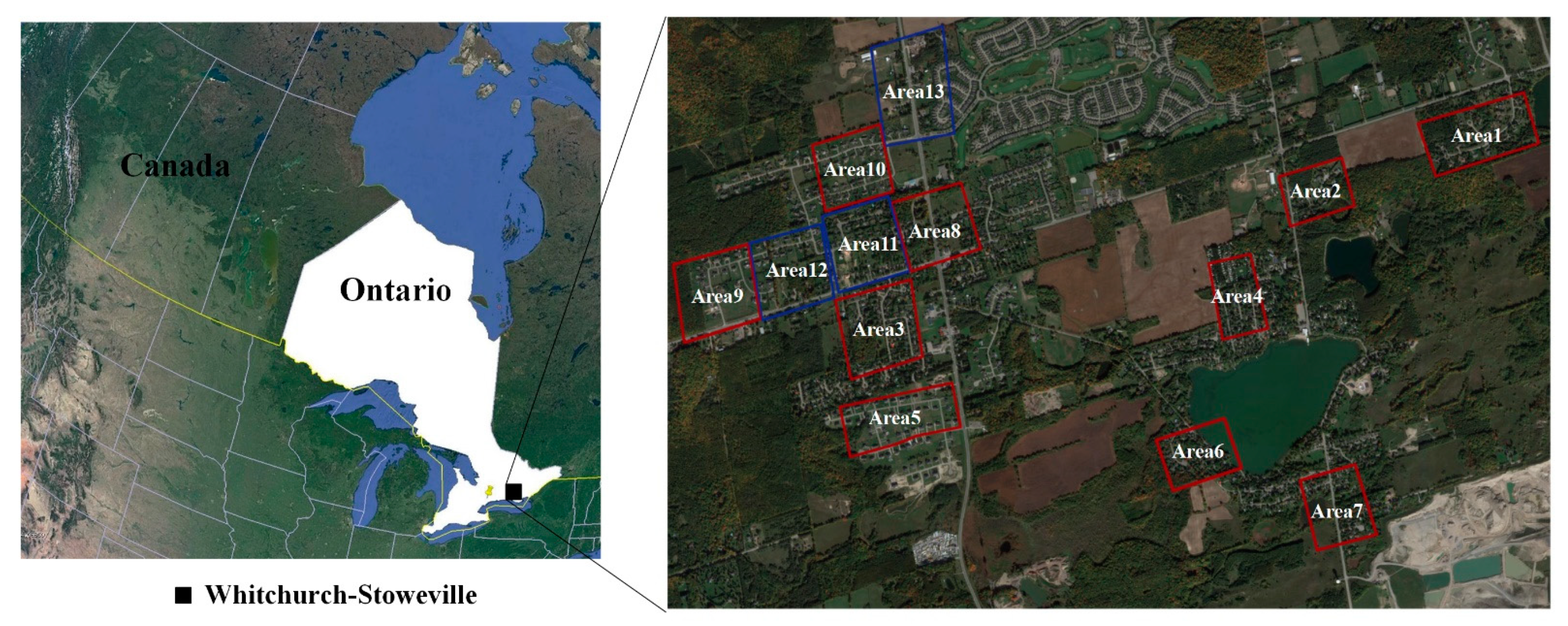
The study area is located at a small town (the center of latitude 43°58′00″, longitude 79°15′00″) in Whitchurch-Stouffville (ON, Canada). As shown in Figure 1, we selected thirteen representative regions containing rich object types, such as asphalt roads, forest and individual trees, open soil and grass, one- and two-story gable roof buildings, industrial buildings, and powerlines. There were nineteen flying strips (ten strips vertically intersecting nine strips), covering an area of about 25 km². Note that, in this study, due to no metadata (such as system parameters and trajectories) provided with the nineteen flying strips, absolute intensity calibration was not performed. The nineteen strips were roughly registered by an iterative closest points (ICP) method. Similarly, because control/reference points were unavailable, the geometric alignment quality was not statistically reported. In this study, as seen in Figure 1, the thirteen study areas (red rectangles for model training and blue rectangles for model testing) were selected for assessing our SE-PointNet++ architecture.

Figure 1. Study areas.

2.2. Data Preprocessing

To generate the required input to our SE-PointNet++ architecture, a two-step data preprocessing (i.e., data fusion and data annotation) is proposed, as shown in Figure 2. Data fusion aims to merge the three individual point clouds of wavelengths (532 nm, 1024 nm, and 1550 nm) into a single point cloud, in which each point contains its coordinates and three-wavelength intensity values. Data annotation aims to manually label the selected thirteen Titan multispectral point cloud regions into several categories of interest and obtain a training dataset for our proposed architecture.

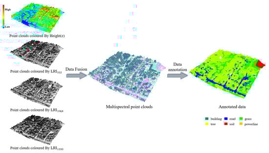
Figure 2. Data preprocessing of the Titan multispectral point clouds.

2.2.1. Data Fusion

The Titan multispectral LiDAR data consist of three independent point clouds, corresponding to three laser wavelengths of 1550 nm, 1064 nm, and 532 nm. The three laser beams were titled by +3.5°, 0°, and +7° from the nadir direction. To fully use the reflectance characteristics of the three wavelengths and improve the point density of the point clouds, the three independent point clouds are first merged into a single, high-density multispectral point cloud, each point of which contains its own intensity and two other assigned intensities from the other wavelengths. In this study, we adopt a 3-D spatial join technique [27] to merge the three independent point clouds. Specifically, among the three point clouds, each single-wavelength point cloud is taken as the reference in turn. Each point of the reference point cloud is processed to find its neighbors in the other two wavelengths of point clouds by a nearest neighbor searching algorithm and then obtains the intensities calculated from the neighbors by a bilinear interpolation method. The search radius is determined according to the point density. For example, as seen in Table 1, for each wavelength, the average point density is about 3.6 points/m², thus, the maximum search distance is set to be 1.0 m to prevent grouping points located on different objects. Note that, for a point in the reference point cloud, if no neighbors are found in one of the other two wavelengths, the intensity value of this wavelength is set to be zero. Finally, the single multispectral point cloud data are preprocessed, each point of which contains its coordinates ($\left[x,y,z\right]$) and its three-wavelength laser intensity (LRI) values $\left[LR{I}_{{\lambda }_{1550}},LR{I}_{{\lambda }_{1064}},LR{I}_{{\lambda }_{532}}\right]$.

2.2.2. Data Annotation

In this study, we select thirteen representative test areas from the collected Titan multispectral point cloud dataset, including six categories (i.e., road, building, grass, tree, soil, and powerline). The total number of points is 8.52 million for the thirteen test areas. By means of the CloudCompare software, six categories were manually labeled point by point. Table 2 shows the number of points of each category in each test area. Each of the selected areas is saved in a separate file, where each point contains seven attributes—coordinates ($x,y,z$), three wavelengths ($LR{I}_{{\lambda }_{1550}},LR{I}_{{\lambda }_{1064}},LR{I}_{{\lambda }_{532}}$), and the category label.

Table 2. Specifications of the Titan system (# represents the number of the points).

	Road (#)	Building (#)	Grass (#)	Tree (#)	Soil (#)	Powerline (#)	Total (#)
area_1	37,956	19,821	207,394	428,525	4549	0	689,245
area_2	24,594	10,408	130,884	259,930	4761	809	431,386
area_3	71,175	78,587	308,337	480,545	13,713	0	952,357
area_4	32,601	45,556	79,891	254,723	7070	493	420,334
area_5	75,710	46,571	347,264	79,966	7189	0	556,700
area_6	32,557	22,786	71,229	207,817	1703	591	336,683
area_7	63,879	39,436	224,173	274,159	1268	2626	605,541
area_8	70,757	25,794	254,340	342,594	6344	4561	704,390
area_9	72,570	33,754	355,467	155,838	9465	2153	629,247
area_10	60,764	61,764	395,228	96,810	31,589	0	655,155
area_11	91,407	41,390	261,218	455,500	16,968	2533	869,016
area_12	94,965	40,941	367,039	252,181	6181	2859	764,166
area_13	117,994	65,040	478,454	198,248	46,380	3075	909,191

2.3. SE-PointNet++ Framewwork

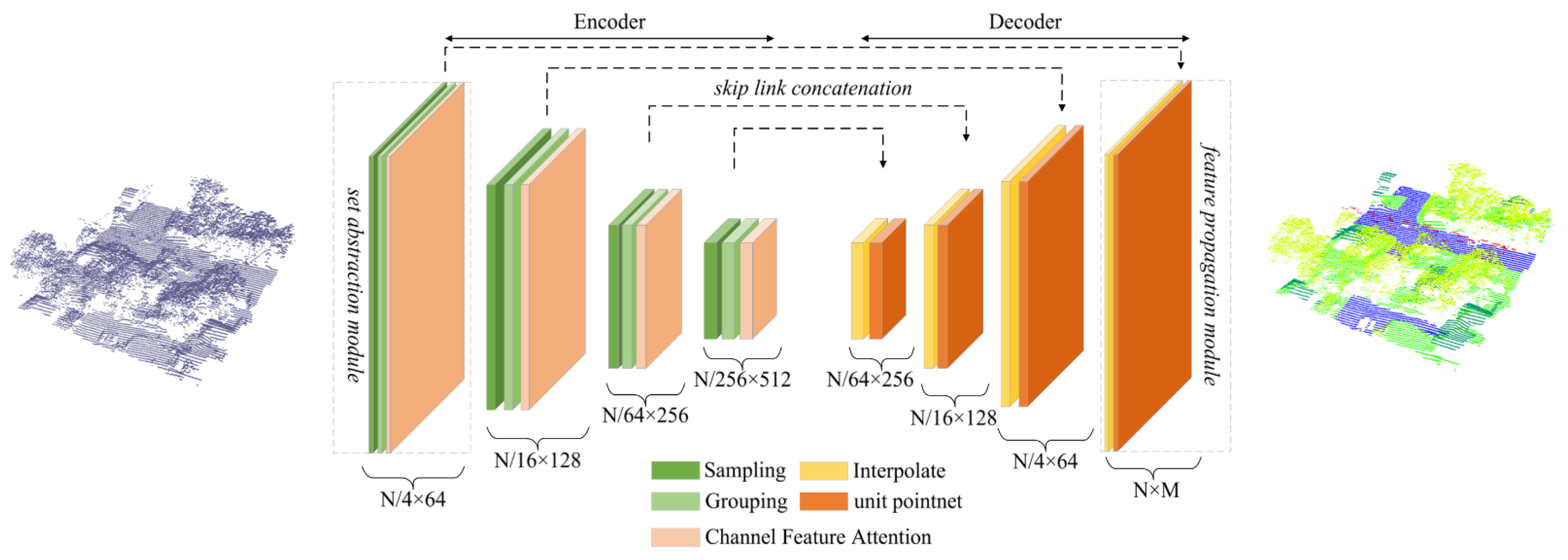
Usually, some of the features learned by deep learning methods, such as PointNet++, might be ineffective for point cloud classification tasks, resulting in high computational costs and a decrease of classification accuracy. Therefore, to emphasize important channels and suppress the channels unconducive to prediction, an improved PointNet++ architecture, termed as SE-PointNet++, is proposed by embedding a Squeeze-and-Excitation block into the PointNet++ architecture. Figure 3 illustrates the SE-PointNet++ framework. As seen in Figure 3, the SE-PointNet++ takes a multispectral LiDAR point cloud (N is the number of points) as the input and outputs an identical-spatial-size point cloud, where each point is labelled with a specific category in an end-to-end manner. The SE-PointNet++ architecture involves an encoder network, a decoder network, and a set of skip link concatenations. The encoder network consists of four set abstraction modules, which recursively extract multi-scale features. The decoder network is operated by four feature propagation modules. The feature propagation modules aim to gradually recover a semantically-strong feature representation to accurately classify the point cloud. The skip link concatenations, to enhance the capability of feature representation, integrate the features selected from the set abstraction modules with the features having the same size in the feature propagation modules. The following subsections first detail the Squeeze-and-Excitation block, followed by a description of the SE-PointNet++.

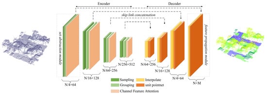
Figure 3. An illustration of the proposed SE-PointNet++.

2.3.1. Squeeze-and-Excitation Block (SE-Block)

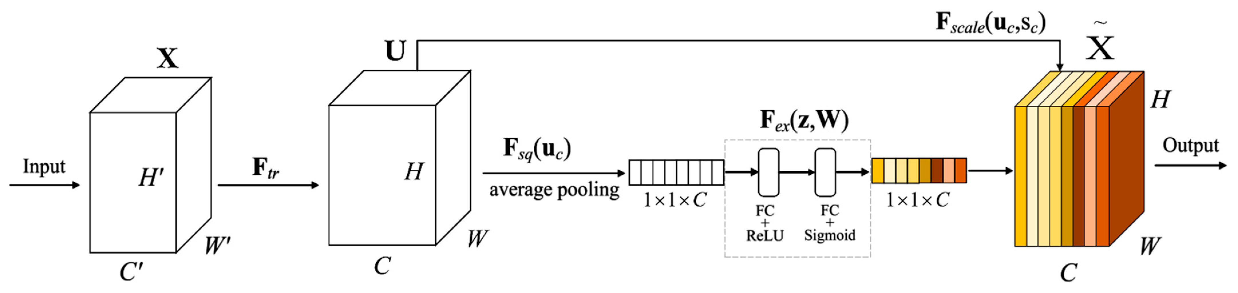
The SE-block aims to improve the expressive ability of the network by explicitly modelling the interdependencies among the channels of its convolutional features of the network without introducing a new spatial dimension for the fusion of the feature channels. Figure 4 illustrates the SE-block structure. Denote $F_{tr}$ as a traditional convolution structure. The SE-block is a computational unit built on a transformation $F_{tr}$, which maps an input $X=\left[x^1, x^2,\dots ,x^{C\prime }\right]$ ($X$ ∈ ${ℝ}^{H\prime \times W\prime \times C\prime }$ , where $H^{\prime }$, $W^{\prime }$, and $C^{\prime }$ are, respectively, the height, width, and channel number of $X$) to feature map $U$ ∈ ${ℝ}^{H\times W\times C}$ (where $H$, $W$ and $C$ are, respectively, the height, width, and channel number of $U$). The $F_{tr}$ transformation is defined as follows:

$$u_c=v_c \ast X={\displaystyle \sum }_{s=1}^{C^{\prime }}{v}_c^s \ast x^s$$

(1)

where ∗ denotes the convolution operation. $v_c=\left[v_c^1, v_c^2,\dots , v_c^{C\prime }\right]$ refers to the parameters of the $c$-th filter. $x^s$ is the $s$-th input of $X$. $v_c^s$ is a 2-D spatial kernel which acts on the corresponding channel of $X$ and represents a single channel of $v_c$. $u_c$∈ ${ℝ}^{H\times W}$ refers to the $c$-th 2-D matrix in $U$. Here, there are two processes—squeeze and excitation.

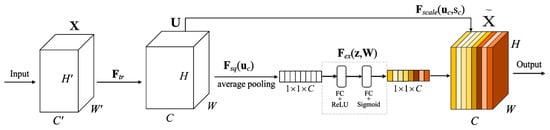
Figure 4. An illustration of the Squeeze-and-Excitation block.

• Squeeze: Global Information Embedding. The squeeze process $F_{sq}\left(u_c\right)$ is designed to compress the spatial information of the feature map by performing a global average pooling for each channel of the feature graph, thereby only channel information is retained. To reduce channel dependencies, the global spatial information is squeezed into a channel descriptor. To this end, a global average pooling is used to generate channel-wise statistics. Formally, a statistic $z$ ∈ ${ℝ}^C$ is generated by shrinking $U$ through its spatial dimensions, $H\times W$. The c-th element of $z$ is calculated by:

  $$z_c=F_{sq}\left(u_c\right)=\frac{1}{H\times W}{\displaystyle \sum }_{i=1}^H{\displaystyle \sum }_{j=1}^W{u}_c\left(i,j\right)$$

  (2)
  Excitation: Adaptive Recalibration. The excitation process $F_{ex}(z,W)$ aims to assign a weight to each element of the $1\times 1\times C$ channel descriptor generated by the squeeze process through two fully connected layers. In this module, a simple gating mechanism is employed with a sigmoid activation to fully capture channel-wise dependencies, which similar to a gating mechanism in recurrent neural network. Specifically, $F_{ex}(z,W)$ exploits the channel-wise interdependencies in a non-mutually exclusive manner by appending two fully connected layers after the squeeze process $F_{sq}\left(u_c\right)$. The outputs of the two fully connected layers are activated using the Rectified Linear Unit (ReLU) and the sigmoid functions, respectively. In this way, the output of the second fully connected layer constitutes a channel-wise attention descriptor, denoted as $s$. The attention descriptor $s$ acts as a weight function to recalibrate the input feature map to highlight the contributions of the informative channels. The attention descriptor $s$ is defined as follows:

  $$s=F_{ex}(z,W)=\sigma \left(g\left(z,W\right)\right)=\sigma \left(W_2\delta \left(W_{1}z\right)\right)$$

  (3)

  where $\delta$ refers to the ReLU function, $W_1$∈${ℝ}^{\frac{C}{r}\times C}$ and $W_2$∈${ℝ}^{C\times \frac{C}{r}}$, $r$ is a reduction ratio in the dimensionality-reduction layer. $\sigma$ refers to the sigmoid function, which limits the importance of each channel to the range of [0, 1], and is multiplied to U in a channel-wise manner to form the input of the next level.
  The final output of the block is obtained by rescaling $U$ with the activations s:

  $${\tilde{x}}_c=F_{scale}\left(u_c,s_c\right)=s_c{u}_c$$

  (4)

  where $\tilde{X}=\left[{\tilde{x}}_1, {\tilde{x}}_2,\dots ,{\tilde{x}}_C\right]$refers to the final output of the block,$s_c$ is the c-th element of $s$. $F_{scale}\left(u_c,s_c\right)$ refers to channel-wise multiplication between scalar $s_c$ and feature map $u_c$ ∈ ${ℝ}^{H\times W}$.

2.3.2. Training Sample Generation

In the collected airborne Titan multispectral LiDAR point clouds, different categories demonstrate different spatial attributes, such as point density due to a top-down data acquisition means. That is, the features learned in the dense sampling areas may not be extended to the sparse sampling areas, and the model trained with the sparse points may not be able to identify fine-grained local structures. Therefore, to address the density inconsistency and sparsity issues of point clouds, a density consistent method is proposed for processing the scenarios with different point densities. The input of the proposed density consistent method is defined as a point set $S=\{p_1,\dots ,p_n | p_i=\left(x,y,z,f \right)\}$where$x,y,z$are the coordinates of the point, and $f$ is the feature vector, such as color and surface normal. We first normalize $S$ to the range of [−1, 1] and output a new point set $\widehat{S}$. Considering the limited GPU capacity, it is impossible to feed an entire training point set directly into the network. We, according to the processed test areas and multispectral LiDAR points, grid the normalized training set ($\widehat{S}$) into a set of blocks using a block size of $0.12\times 0.12$ m² without overlapping, each of which contains a different number of points. To obtain a fixed number of samples for each point block, a farthest point sampling (FPS) algorithm is used to down-sample it with a given number sample size, $N$. Note that, for each point block, the higher the number of the training samples, the more the information learned by the proposed architecture. However, computational performance should be taken into account when the number of samples is defined. Due to point density inconsistency, some point blocks might contain few points with the number of sampling points smaller than $N$. Therefore, data interpolation is required to obtain the defined number size of sampling points.

2.3.3. SE-PointNet++

After the generation of the training samples, the $N$ multispectral LiDAR points with six attributes (coordinates ($x,y,z$) and three-wavelength intensities ($LR{I}_{{\lambda }_{1550}},LR{I}_{{\lambda }_{1064}},LR{I}_{{\lambda }_{532}}$)) are directly input into our SE-PointNet++ architecture, which involves an encoder network, a decoder network, and a set of skip link concatenations. The encoder network consists of four set abstraction modules to recursively extract multi-scale features at the scale of {1/4, 1/16, 1/64, 1/256} with regard to the input point cloud with the point number of N. Figure 5 shows the first set abstraction module. Specifically, a set abstraction module takes an $N\times 6$ matrix as the input and outputs an $N/4\times 64$ matrix of $N/4$ subsampled points with $64-dimensional$ feature vectors summarizing the local contextual information. As seen in Figure 5, the set abstraction module in the encoder network consists of a Sampling layer, a Grouping layer, and a Channel Feature Attention layer. Firstly, the sampling layer defines the $N/4$ centroids of local regions by selecting a set of points through an iterative FPS algorithm. Given the input points $\left\{x_1,x_2,\dots ,x_n\right\}$, the FPS selects a subset of points $\left\{x_{i_1},x_{i_2},\dots ,x_{i_m}\right\}$, such that $x_{i_j}$ is the fastest distant point from the remaining point set $\left\{x_{i_1},x_{i_2},\dots ,x_{i_{j-1}}\right\}$. The centroids of the sampling layer are 1/4 times of the input points each time. Afterwards, a grouping layer is used to construct the corresponding local regions by searching for the neighboring points around the $N/4$ centroids by a ball query algorithm. For each centroid, via the ball query algorithm, all neighboring points are found within a given radius, from which $K$ points are randomly selected to construct a local region ($K$ is set to 32 in this study). After the implementation of the sampling and grouping layers, the multispectral LiDAR points are then sampled into $N/4$ point sets, each of which contains 32 points with their 6 attributes. The output involves a group of point sets with the size of $N/4\times 32\times 6$. Subsequently, we encode these local regions into feature vectors via our Channel Feature Attention layer. For each point, we extract its features by multi-layer perceptrons (MLPs), and emphasize its important features and suppress its unimportant channels by the SE block. Specifically, in the SE block, each channel of the $N/4$ points is squeezed via a max-pooling, and then its weight value is calculated and normalized to the range of [0, 1] by the two MLP layers and sigmoid function. The higher the weight value, the more important the channel. Finally, the important channels with higher weight values are then excited. To avoid the situation of missing features when the weight is close to zero, a short connection is used to connect the features before and after the channel feature attention layer. Because there exist different dimensions of the learned features before and after the channel feature attention layer, convolution operation is performed to match their dimensions in the shortcut connection.

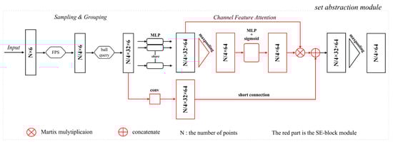
Figure 5. An illustration of the set abstraction module.

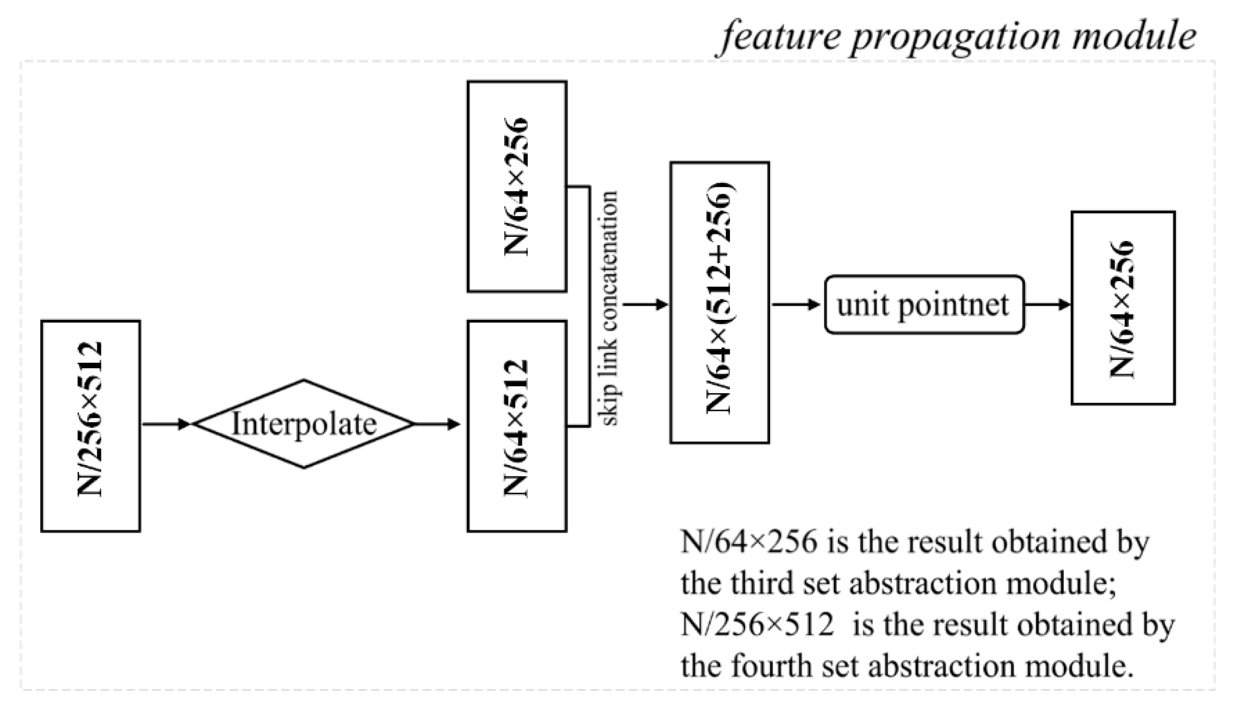
The decoder network includes four feature propagation modules, which gradually recover a semantically-strong feature representation to produce a high-quality classified point cloud. Figure 6 shows an example of the feature propagation module. As illustrated in Figure 6, the output data size of the encoder is $N/256\times 512$ (where, $512$ is the dimension of features), which contains more useful channel feature information. To propagate the learned features from the sampled points to the original points, interpolation is first employed through an inverse distance weighting within the feature propagation module. The point features are propagated from $N/256\times 512$ points to $N/64$ points, where $N/64$ and $N/256$ are the point sets of the input and the output of the fourth set abstraction module.

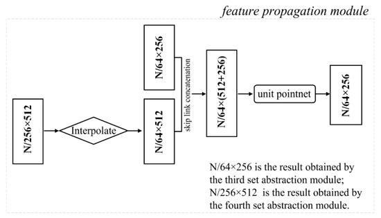
Figure 6. An illustration of the feature propagation module.

To enhance the capability of the feature representation, the interpolated features on the $N/64$ points are then concatenated with the skip linked point features from the set abstraction modules via the skip link concatenations. Then, to capture features from the coarse-level information, the concatenated features are passed through a “unit pointnet”, similar to 1×1 convolution in CNNs. A few shared fully connected and ReLU layers update the feature vector of each point. The process is repeated until the features have been propagated to the original point set.

3. Results

To assess the performance of the SE-PointNet++ on multispectral point cloud classification, we conducted several groups of experiments on the Titan multispectral LiDAR Data.

3.1. Experimental Setting

We implemented all tests in the framework of Pytorch1.5.0 and trained them with GTX 1080Ti GPU. Each point of the Titain multispectral LiDAR data contained its coordinates ($\left[x,y,z\right]$), three-wavelength intensity values $\left[LR{I}_{{\lambda }_{1550}},LR{I}_{{\lambda }_{1064}},LR{I}_{{\lambda }_{532}}\right]$ and the category label. The number of sampling points, $N$, was set to be 4096 points. The number of neighbors, $K$, was set to be 32 when calculating low-dimensional prior $G_{\phi }$. Parameters, i.e., learning rate, batch size, decay rate, optimizer, and max epoch, were set to be 0.001, 8, 10⁻⁴, Adam, and 200, respectively. Among the selected thirteen test areas, the first ten areas (area_1 to area_10, about 70% of the data) were used as the training sets, and the remaining (area_11 to area_13, about 30% of the data) as the test sets.

3.2. Evaluation Metrics

The following evaluation metrics were used to quantitatively compare and analyze the multispectral LiDAR point cloud classification results. These metrics include overall accuracy (OA) [42], mean intersection over union (mIoU) [43], Kappa coefficient (Kappa) [44], and F₁-score [45]. The metrics are presented as follows:

$$\mathrm{OA}=\frac{tp+tn}{tp+tn+fp+fn}$$

(5)

$$\mathrm{mIoU}=\frac{tp}{tp+fp+fn}$$

(6)

$$\mathrm{Kappa}=\frac{\mathrm{OA}-p_e}{1-p_e}$$

(7)

$$p_e=\frac{\left(tp+tn\right)\times \left(tp+fp\right)}{{\left(tp+tn+fp+fn\right)}^2}+\frac{\left(tn+fp\right)\times \left(tn+fn\right)}{{\left(tp+tn+fp+fn\right)}^2}$$

(8)

$$F_1-score=2\times \frac{precision\times recall}{precision+recall}$$

(9)

$$precision=\frac{tp}{tp+fp}$$

(10)

$$recall= \frac{tp}{tp+fn}$$

(11)

where $tp$ is the number of true positives, $tn$ is the number of true negatives, $fp$ is the number of false positives, and $fn$ is the number of false negatives.

3.3. Overall Performance

To evaluate the point cloud classification performance of the SE-PointNet++, we applied it to the Titan multispectral LiDAR data. Figure 7 shows the point cloud classification results of our SE-PointNet++ architecture. Visual inspection demonstrates that most categories (see Figure 7a–c)) were correctly classified, compared with the ground truth (see Figure 7d–f). Specifically, the road, grass, tree, and building points in the three areas were all clearly classified. However, some soil points were misclassified as the grass points. The reason behind this phenomenon might be the similar topological features and geographical distributions of these two categories. In addition, some powerline points were misclassified as the tree points, which may also be caused by the mixing and lack of obvious boundaries between the two categories.

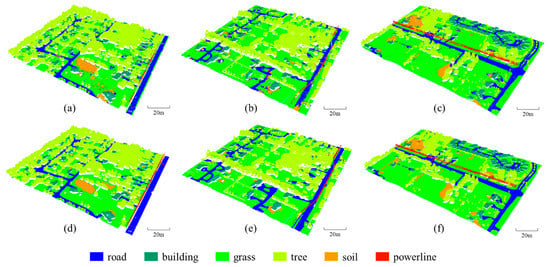
Figure 7. Comparison results of the SE-PointNet++. (a–c) are the point cloud classification results of the SE-PointNet++. (d–f) represent the ground truth of the three test areas, respectively.

To statistically assess the point cloud classification performance of our network, the classification confusion matrix was calculated and listed in Table 3. As seen in this table, our proposed architecture obtained the OA higher than 70% for five categories, i.e., road, building, grass, tree, and powerline. Particularly, the grass and tree categories achieved higher classification accuracies with an OA of 94.70% and 97.09%, respectively. One of the facts is that, in the Titan multispectral LiDAR system, three channels, i.e., 532 nm, 1024 nm, and 1550 nm, provide rich vegetation information. In feature engineering-based methods, some vegetation indices can be derived from the three channels, improving the classification accuracies of grass and tree. Our architecture achieved a modest classification performance on soil with an OA of 52.45%. Most soil points were misclassified as grass ones.

Table 3. The point cloud classification confusion matrix of the SE-PointNet++, (# represents the number of the points).

Categories	Road (#)	Building (#)	Grass (#)	Tree (#)	Soil (#)	Powerline (#)
road	166,311	532	57,035	165	12,460	0
building	367	93,747	561	14,684	0	110
grass	14,297	274	842,690	3429	29,195	0
tree	247	12,998	5208	670,476	227	1415
soil	8810	324	9581	80	20,733	0
powerline	0	752	0	1714	0	5850
OA (%)	70.32	85.64	94.70	97.09	52.45	70.35

The reason behind this phenomenon might be the similarities of the spatial distributions and topological characteristics between soil and grass. Comparatively, although the study area contains few points of powerline, our presented SE-PointNet++ correctly recognized the powerline points from the data due to the geometrical and distribution characteristics of powerline. Due to the use of LiDAR elevation information, objects at different elevations can be easily differentiated, for example, only 697 road points (account for 0.3% of all points) were misclassified as other high-rise categories, such as building, tree, and powerline. Specifically, 928 building points (0.85%) were misclassified as road and grass points; 404 soil points (1%) were misclassified as building and tree points.

3.4. Comparative Experiments

To fairly demonstrate the robustness and effectiveness of our architecture, we compared it with other representative point-based deep learning models, including PointNet [35], PointNet++ [36], DGCNN [37], GACNet [38], and RSCNN [39]. Although these models have achieved excellent performance on point cloud classification and semantic segmentation, they have not been tested on large-scale multispectral LiDAR data containing complex urban geographical features. A quantitative comparison between the SE-PointNet++ and the other five models are listed in Table 4.

Table 4. A comparative point cloud classification results of our SE-PointNet++ with other five established deep learning modules under three test areas (11–13).

Model	OA (%)	mIoU (%)	F1-Score (%)	Kappa
PointNet [35]	83.79	44.28	46.68	0.73
PointNet++ [36]	90.09	58.60	70.13	0.84
DGCNN [37]	91.36	51.04	66.17	0.86
GACNet [38]	89.91	55.14	69.64	0.84
RSCNN [39]	90.99	56.10	70.23	0.86
SE-PointNet++	91.16	60.15	73.14	0.86

As shown in Table 4, in terms of the point cloud classification accuracy, the PointNet achieved the worst point cloud classification with an OA of 83.79%. The reason behind this phenomenon is that the PointNet neglected the points-to-points spatial neighboring relations, which contained fine-grained structural information for segmentation. The GACNet behaved modestly with an OA of 89.91 %. Due to the integration of an attention scheme with graph attention convolution, the GACNet was capable of adapting kernel shapes to dynamically adapt to the structures of the objects, thereby improving the quality of feature representation for accurate point cloud classification. The PointNet++, DGCNN, RSCNN, and our SE-PointNet++ outperformed the aforementioned two methods with the OA of over 90.0%. For the DGCNN, benefiting from the local neighborhood graphs constructed by EdgeConv, similar local shapes can be easily captured, which contributed to the improvement of feature representation. RSCNN, via relation-shape convolutions, produced geometric relationships of points to obtain discriminative shape awareness, thereby achieving a good point cloud classification performance. However, these methods performed ineffectively with a high cost of data structuring, which limits their abilities to generalize complex scenarios. PointNet++ used a hierarchical structure to extract the local information of points, thereby achieving a better point cloud classification result. As seen from the other evaluation metrics, the SE-PointNet++ achieved the best scores of mIoU (62.15%), F₁-score (73.14%) and Kappa coefficient (0.86). The introduction of the SE-blocks that fused local and global features of points contributed to fine-grained information acquisition. As a result, the SE-PointNet++ achieved with the mIoU value increased up to 60.15%. Note that the six categories in the thirteen test areas were unevenly distributed. As seen in Table 2, the number of points greatly changed from one category to another, leading to that the categories with sufficient points achieved a good point cloud classification performance, while the categories with few points achieved a poor point cloud classification performance.

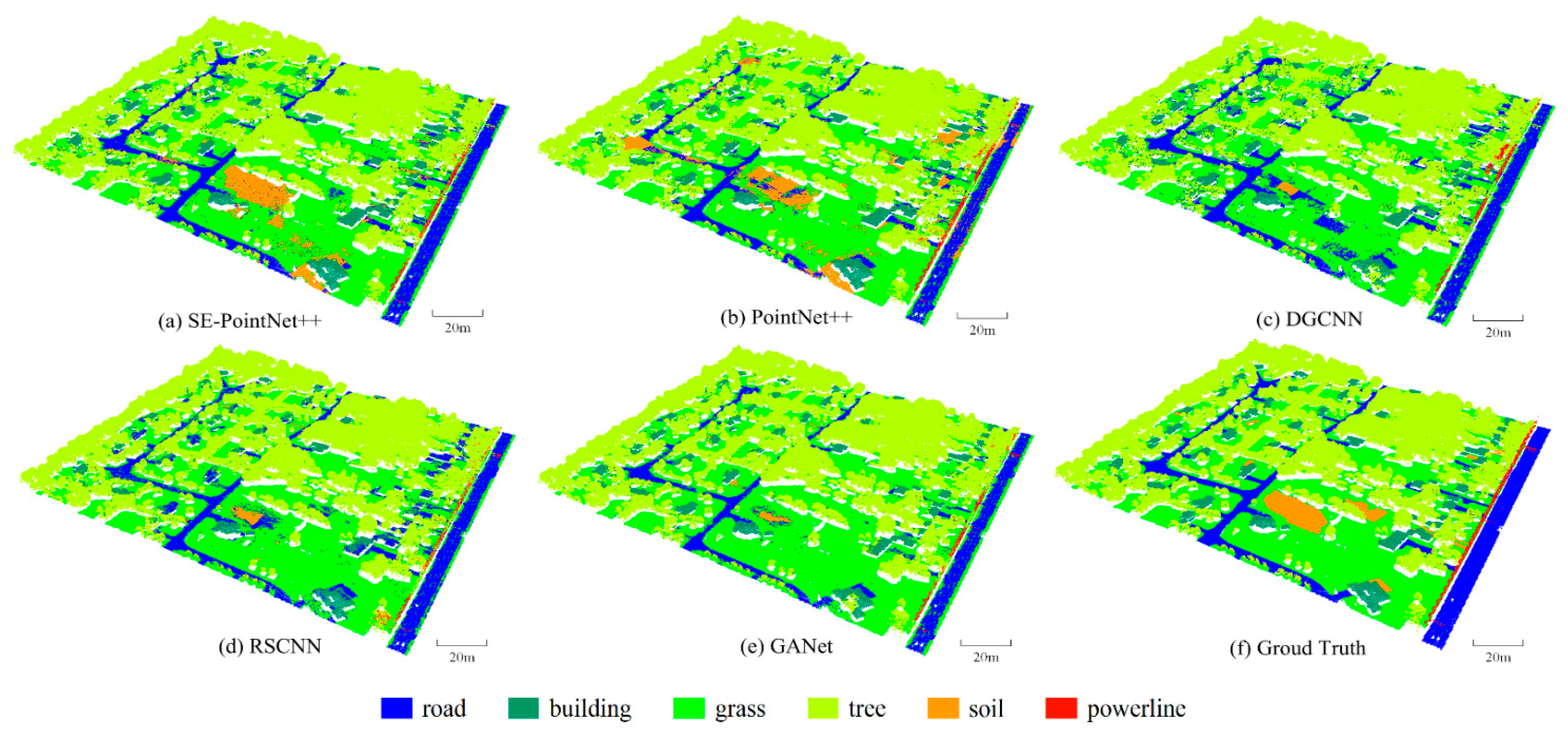
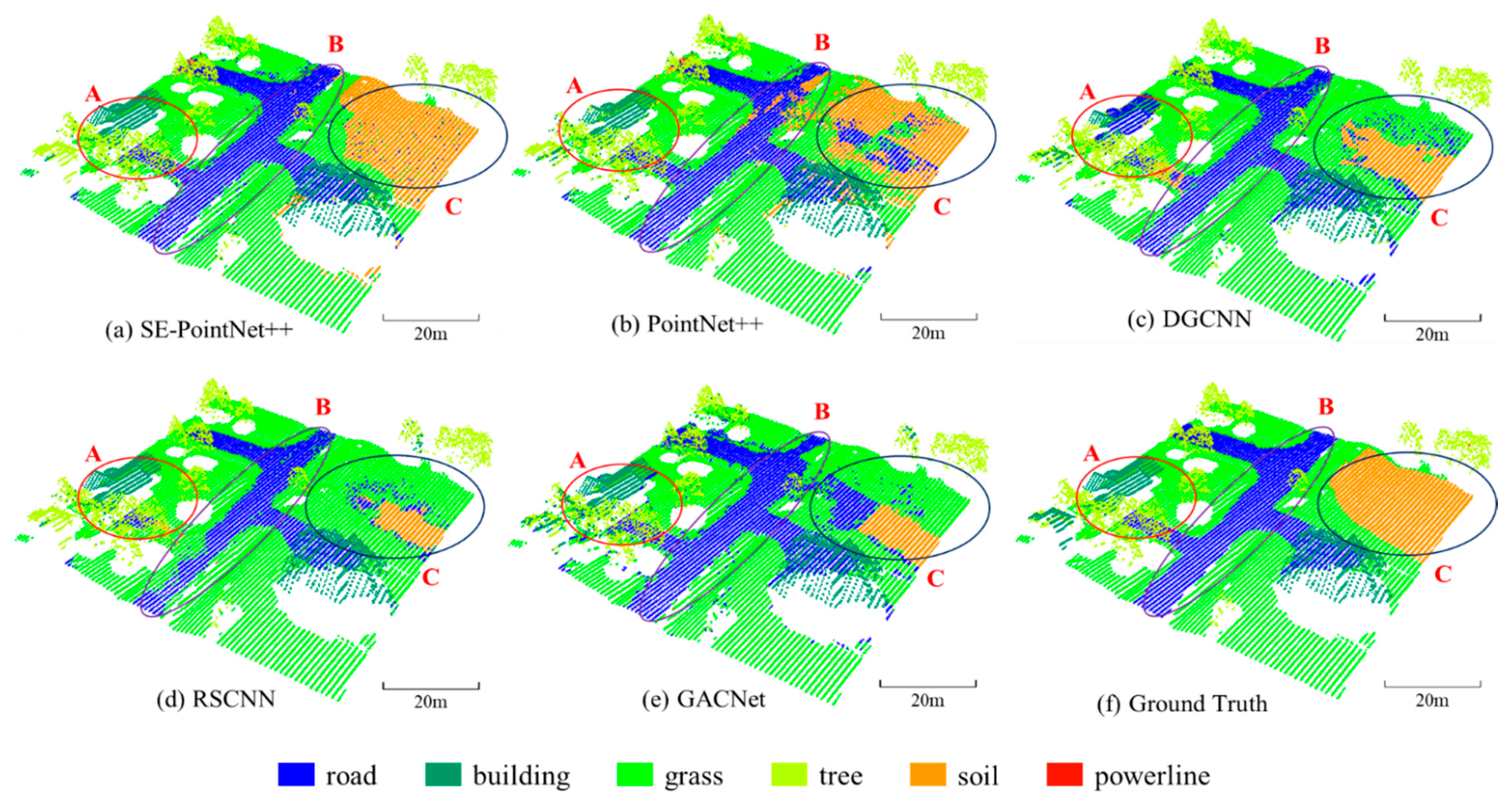
Figure 8 shows the comparative point cloud classification results of the area_11 test area. Figure 9 shows a close-up view of the comparative point cloud classification results. Three oval-shaped regions (i.e., Regions A, B, and C) were highlighted for further comparison. Visual inspection of Region A indicates that the DGCNN, RSCNN, and GACNet models misclassified most bare soil points as grass ones. This is due to their similar topological features and geographical distributions. The three models heavily relied on the geometric relationships between points. Specifically, DGCNN used EdgeConv as a feature extraction layer to leverage neighborhood structures in both point and feature spaces. RSCNN and GACNet used relation-shape convolution and graph attention convolution to encode the geometric relationship of points, respectively. Similarly, as seen in Region C, for the DGCNN , RSCNN and GACNet classification results, some bare soil points were misclassified as road and grass points. Although the PointNet++ achieved satisfactory classification accuracy of the soil category (see Table 4 and Region B in Figure 9), some road points were misclassified as bare soil ones. However, as seen from Region B, our SE-PointNet++ model accurately predicted road points. This is due to the SE-block embedded in the feature extraction process to enhance important channels and suppress useless channels, thereby our architecture achieved better classification accuracies for the soil, road, and grass categories.

Figure 8. Illustration of the comparative point cloud classification results. (a) SE-PointNet++, (b) PointNet++, (c) DGCNN, (d) RSCNN, (e) GACNet and (f) Ground truth.

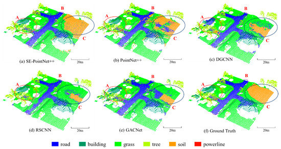
Figure 9. Illustration of a close-up view of the comparative point cloud classification results. (a) SE-PointNet++, (b) PointNet++, (c) DGCNN, (d) RSCNN, (e) GACNet and (f) Ground truth.

4. Discussion

4.1. Parameter Analysis

In the proposed SE-PointNet++, there are two parameters, input data and the number of sampling points, $N$. We designed the following experiments to investigate (1) the superiority of the multispectral LiDAR data, and (2) the feasibility of SE-PointNet++ to the selection of the parameter $N$.

4.1.1. Input Data

To assess the superiority of the fused multispectral LiDAR data to point cloud classification, we input different types of data into the proposed SE-PointNet++ architecture. Five experiments were conducted to investigate the input data types: (1) only geometrical data without any intensities (i.e., Case 1-1), (2) 1550 nm LiDAR data (i.e., Case 1-2), (3) 1064 nm LiDAR data (i.e., Case 1-3), (4) 532 nm LiDAR data (i.e., Case 1-4), and (5) multispectral LiDAR data (i.e., Case 1-5). In this group of experiments, $N$ was set to be 4096. Table 5 shows the average experimental results for the selected 13 test areas.

Table 5. Point cloud classification results with the different input data under three test areas (11–13).

Exp. No.	Input Data Type	OA (%)	mIoU (%)	F1-Score (%)	Kappa
Case 1-1	only geometrical data	88.91	52.55	62.41	0.83
Case 1-2	1550nm-wavelength LiDAR data	82.48	51.50	62.33	0.72
Case 1-3	1064nm-wavelength LiDAR data	90.47	58.09	68.40	0.85
Case1-4	532nm-wavelength LiDAR data	84.12	49.53	61.05	0.754
Case1-5	multispectral LiDAR data	91.16	60.15	73.14	0.86

As seen from Table 5, the point cloud classification accuracies of the 532 nm LiDAR data are very close to those of the 1550 nm LiDAR data. Compared with the other two single-wavelength data, the 1064nm LiDAR data achieved better point cloud classification accuracies with an OA of 90.47%, an mIoU of 58.09%, an F₁-Score of 68.40%, and a Kappa coefficient of 0.8503. The multispectral LiDAR data achieved the best point cloud classification performance by the OA improvement from 1% to 9%, the mIoU improvement from 1% to 9%, the F₁-score improvement from 5% to 14%, and the Kappa coefficient improvement from 0.01 to 0.14.

4.1.2. Number of Sampling Points

To investigate the effect of the number of sampling points on point cloud classification results using the Titan multispectral LiDAR data, we varied $N$ from 4096, 2048, 1024, 512, 128, to 32. Table 6 shows the experimental results of the six categories. As shown in Table 6, the point cloud classification accuracies dramatically decreased when the number of the sampling points decreased from 4096 to 32. Our architecture achieved its best performance when $N$ was set to be 4096. The main reason for this situation is that the less the number of sampling points, the less the features being represented for each category. Of course, the larger the number of points, the better the point cloud classification accuracy. However, due to the computation capacity limitation of the computer being used, the number of sampling points cannot be set extensively large in this study. As such, in our study, the better point cloud classification accuracies were obtained when $N$= 4096.

Table 6. Poind cloud classification results with different numbers of sampling points (N) under three test areas (11–13).

Exp. No.	Number of Sampling Points	OA (%)	mIoU (%)	F1-Score (%)	Kappa
Case 2-1	4096	91.16	60.15	73.14	0.86
Case 2-2	2048	90.96	60.05	73.15	0.86
Case 2-3	1024	89.08	58.93	69.92	0.83
Case 2-4	512	89.18	57.19	67.88	0.83
Case 2-5	128	87.02	50.88	61.13	0.80
Case 2-6	32	84.41	44.03	52.28	0.76

4.2. Analysis of Imbalanced Data Distribution

As seen in Table 4, although our SE-PointNet++ achieved relatively better performances than most of the comparative methods. In particular, DGCNN obtained the comparable performance with the SE-PointNet++, and even outperformed the SE-PointNet++ in terms of the overall accuracies. We believe that the main reason for this phenomenon is the distribution imbalance of the categories in the study area. As shown in Table 2, the six categories are not balanced in distribution. For example, the data set contains 3.48 million tree points, while twenty thousand powerline points. This imbalanced point distribution degraded the overall point cloud classification accuracies. To fairly evaluate the performance, we balanced the points of all categories to a certain extent by an oversampling and undersampling method. The experimental results are shown in Table 7.

Table 7. Point cloud classification results obtained by different architectures.

Model	OA (%)	mIoU (%)	F1-Score (%)	Kappa
PointNet [35]	68.89	45.08	42.94	0.57
PointNet++ [36]	79.08	55.83	68.96	0.75
DGCNN [37]	84.19	52.53	66.9	0.78
GACNet [38]	80.66	45.32	59.24	0.74
RSCNN [39]	81.21	55.37	68.18	0.75
SE-PointNet++	85.07	58.17	71.45	0.80

Comparatively, our SE-PointNet++ showed a significant improvement compared with the other methods with an OA of 85.07%, an mIoU of 58.17%, an F₁-score of 71.45%, and a Kappa coefficient of 0.80. Through the above experiments and discussion, we confirmed that the SE-PointNet++, that is, the integration of SE-blcok with PointNet++, performed positively and effectively in improving the quality of the multispectral LiDAR point cloud classification results.

5. Conclusions

The multispectral LiDAR point cloud data contain both geometrical and multi-wavelength information, which contributes to identifying different land-cover categories. In this study, we proposed an improved PointNet++ architecure, named SE-PointNet++, by integrating an SE attention mechanism into the PointNet++ for the multispectral LiDAR point cloud classification task. First, data preprocessing was performed for data merging and annotation. A set of samples were obtained by the FPS point sampling method. By embedding the SE-block into the PointNet++, the SE-PointNet++ is capable of both extracting local geometrical relationships among points from unevenly sampled data, and strengthening important feature channels simultaneously, which improves multispectral LiDAR point cloud classification accuracies.

We have tested the SE-PointNet++ on the Titan airborne multispectral LiDAR data. The dataset was classified into six land-cover categories: road, building, grass, tree, soil, and powerline. Quantitative evaluations showed that our SE-PointNet++ achieved a classification performance with the OA, mIoU, F₁-score, and Kappa coefficient of 91.16%, 60.15%, 73.14%, and 0.86 of, respectively. In addition, the comparative studies with five established methods also confirmed that the SE-PointNet++ was feasible and effective in 3-D multispectral LiDAR point cloud classification tasks.

References

- Wen, C.; Yang, L.; Li, X.; Peng, L.; Chi, T. Directionally constrained fully convolutional neural network for airborne LiDAR point cloud classification. ISPRS J. Photogramm. Remote Sens. 2020, 162, 50–62. [Google Scholar] [CrossRef] [Green Version]
- Li, W.; Wang, F.; Xia, G. A geometry-attentional network for ALS point cloud classification. ISPRS J. Photogramm. Remote Sens. 2020, 164, 26–40. [Google Scholar] [CrossRef]
- Yan, W.Y.; Shaker, A.; El-Ashmawy, N. Urban land cover classification using airborne LiDAR data: A review. Remote Sens. Environ. 2015, 158, 295–310. [Google Scholar] [CrossRef]
- Antonarakis, A.S.; Richards, K.S.; Brasington, J. Object-based land cover classification using airborne LIDAR. Remote Sens. Environ. 2008, 112, 2988–2998. [Google Scholar] [CrossRef]
- Blackman, R.; Yuan, F. Detecting long-term urban forest cover change and impacts of natural disasters using high-resolution aerial images and LiDAR data. Remote Sens. 2020, 12, 1820. [Google Scholar] [CrossRef]
- Huang, M.J.; Shyue, S.W.; Lee, L.H.; Kao, C.C. A knowledge-based approach to urban feature classification using aerial imagery with lidar data. Photogramm. Eng. Remote Sens. 2008, 74, 1473–1485. [Google Scholar] [CrossRef] [Green Version]
- Chen, Y.; Su, W.; Li, J.; Sun, Z. Hierarchical object oriented classification using very high resolution imagery and LIDAR data over urban areas. Adv. Space Res. 2009, 43, 1101–1110. [Google Scholar] [CrossRef]
- Zhou, K.; Ming, D.; Lv, X.; Fang, J.; Wang, M. Cnn-based land cover classification combining stratified segmentation and fusion of point cloud and very high-spatial resolution remote sensing image data. Remote Sens. 2019, 11, 2065–2094. [Google Scholar] [CrossRef] [Green Version]
- Yokoya, N.; Ghamisi, P.; Xia, J.; Sukhanov, S.; Heremans, R.; Tankoyeu, I.; Bechtel, B.; Saux, B.; Moser, G.; Tuia, D. Open data for global multimodal land use classification: Outcome of the 2017 IEEE GRSS Data Fusion Contest. IEEE J. Sel. Top. Appl. Earth Obs. Remote Sens. 2018, 11, 1363–1377. [Google Scholar] [CrossRef] [Green Version]
- Xu, Y.; Du, B.; Zhang, L.; Cerra, D.; Pato, M.; Carmona, E.; Prasad, S.; Yokoya, N.; Hänsch, R.; Saux, B. Advanced multi-sensor optical remote sensing for urban land use and land cover classification: Outcome of the 2018 IEEE GRSS data fusion contest. IEEE J. Sel. Top. Appl. Earth Obs. Remote Sens. 2019, 12, 1709–1724. [Google Scholar] [CrossRef]
- Gong, W.; Sun, J.; Shi, S.; Yang, J.; Du, L.; Zhu, B.; Song, S. Investigating the potential of using the spatial and spectral information of multispectral LiDAR for object classification. Sensors 2015, 15, 21989–22002. [Google Scholar] [CrossRef] [Green Version]
- Wallace, A.M.; McCarthy, A.; Nichol, C.J.; Ren, X.; Morak, S.; Martinez-Ramirez, D.; Woodhouse, I.; Buller, G.S. Design and evaluation of multispectral LiDAR for the recovery of arboreal parameters. IEEE Trans. Geosci. Remote Sens. 2014, 52, 4942–4954. [Google Scholar] [CrossRef] [Green Version]
- Hartzell, P.; Glennie, C.; Biber, K.; Khan, S. Application of multispectral LiDAR to automated virtual outcrop geology. ISPRS J. Photogramm. Remote Sens. 2014, 88, 147–155. [Google Scholar] [CrossRef]
- Shi, S.; Song, S.; Gong, W.; Du, L.; Zhu, B.; Huang, X. Improving backscatter intensity calibration for multispectral LiDAR. IEEE Geosci. Remote Sens. Lett. 2015, 12, 1421–1425. [Google Scholar] [CrossRef]
- Li, D.; Shen, X.; Yu, Y.; Guan, H.; Li, D. Building extraction from airborne multi-spectral lidar point clouds based on graph geometric moments convolutional neural networks. Remote Sens. 2020, 12, 3186. [Google Scholar] [CrossRef]
- Teo, T.A.; Wu, H.M. Analysis of land cover classification using multi-wavelength LiDAR system. Appl. Sci. 2017, 7, 663. [Google Scholar] [CrossRef] [Green Version]
- Zou, X.; Zhao, G.; Li, J.; Yang, Y.; Fang, Y. 3D land cover classification based on multispectral lidar point clouds. ISPRS Int. Arch. Photogramm. Remote Sens. Spat. Inf. Sci. 2016, 41, 741–747. [Google Scholar] [CrossRef] [Green Version]
- Matikainen, L.; Karila, K.; Hyyppä, J.; Litkey, P.; Puttonen, E.; Ahokas, E. Object-based analysis of multispectral airborne laser scanner data for land cover classification and map updating. ISPRS J. Photogramm. Remote Sens. 2017, 128, 298–313. [Google Scholar] [CrossRef]
- Bakuła, K.; Kupidura, P.; Jełowicki, L. Testing of land cover classification from multispectral airborne laser scanning data. ISPRS Arch. 2016, 41, 161–169. [Google Scholar]
- Fernandez-Diaz, J.C.; Carter, W.E.; Glennie, C.; Shrestha, R.L.; Pan, Z.; Ekhtari, N.; Singhania, A.; Hauser, D.; Sartori, M. Capability assessment and performance metrics for the titan multispectral mapping lidar. Remote Sens. 2016, 8, 936. [Google Scholar] [CrossRef] [Green Version]
- Huo, L.Z.; Silva, C.A.; Klauberg, C.; Mohan, M.; Zhao, L.J.; Tang, P.; Hudak, A.T. Supervised spatial classification of multispectral LiDAR data in urban areas. PLoS ONE 2018, 13, e0206185. [Google Scholar] [CrossRef]
- Matikainen, L.; Karila, K.; Litkey, P.; Ahokas, E.; Hyyppä, J. Combining single photon and multispectral airborne laser scanning for land cover classification. ISPRS J. Photogramm. Remote Sens. 2020, 164, 200–216. [Google Scholar] [CrossRef]
- Esteva, A.; Robicquet, A.; Ramsundar, B.; Kuleshov, V.; DePristo, M.; Chou, K.; Cui, C.; Corrado, G.; Thrun, S.; Dean, J. A guide to deep learning in healthcare. Nat. Med. 2019, 25, 24–29. [Google Scholar] [CrossRef]
- Bello, S.A.; Yu, S.; Wang, C.; Adam, J.; Li, J. Review: Deep learning on 3d point clouds. Remote Sens. 2020, 12, 1729. [Google Scholar] [CrossRef]
- Pan, S.; Guan, H.; Yu, Y.; Li, J.; Peng, D. A comparative land-cover classification feature study of learning algorithms: DBM, PCA, and RF using multispectral LiDAR data. IEEE J. Sel. Top. Appl. Earth Obs. Remote Sens. 2019, 12, 1314–1326. [Google Scholar] [CrossRef]
- Yu, Y.; Guan, H.; Li, D.; Gu, T.; Wang, L.; Ma, L.; Li, J. A hybrid capsule network for land cover classification using multispectral LiDAR data. IEEE Geosci. Remote Sens. Lett. 2019, 17, 1263–1267. [Google Scholar] [CrossRef]
- Wichmann, V.; Bremer, M.; Lindenberger, J.; Rutzinger, M.; Georges, C.; Petrini-Monteferri, F. Evaluating the potential of multispectral airborne Lidar for topographic mapping and land cover classification. ISPRS Ann. Photogramm. Remote Sens. Spat. Inf. Sci. 2015, 2, 113–119. [Google Scholar] [CrossRef] [Green Version]
- Morsy, S.; Shaker, A.; El-Rabbany, A.; LaRocque, P.E. Airborne multispectral lidar data for land-cover classification and land/water mapping using different spectral indexes. ISPRS Ann. Photogramm. Remote Sens. Spat. Inf. Sci. 2016, 3, 217–224. [Google Scholar] [CrossRef] [Green Version]
- Sun, J.; Shi, S.; Chen, B.; Du, L.; Yang, J.; Gong, W. Combined application of 3D spectral features from multispectral LiDAR for classification. In Proceedings of the 2017 IEEE International Geoscience and Remote Sensing Symposium (IGARSS 2017), Fort Worth, TX, USA, 23–28 July 2017; pp. 2756–2759. [Google Scholar]
- Ekhtari, N.; Glennie, C.; Fernandez-Diaz, J.C. Classification of multispectral LiDAR point clouds. In Proceedings of the 2017 IEEE International Geoscience and Remote Sensing Symposium (IGARSS 2017), Fort Worth, TX, USA, 23–28 July 2017; pp. 2756–2759. [Google Scholar]
- Ekhtari, N.; Glennie, C.; Fernandez-Diaz, J.C. Classification of airborne multispectral lidar point clouds for land cover mapping. IEEE J. Sel. Top. Appl. Earth Obs. Remote Sens. 2018, 11, 2756–2759. [Google Scholar] [CrossRef]
- Miller, C.I.; Thomas, J.J.; Kim, A.M.; Metcalf, J.P.; Olsen, R.C. Application of image classification techniques to multispectral lidar point cloud data. In Proceedings of the Laser Radar Technology and Applications XXI, Baltimore, MA, USA, 13 May 2016; p. 98320X. [Google Scholar]
- Morsy, S.; Shaker, A.; El-Rabbany, A. Multispectral LiDAR data for land cover classification of urban areas. Sensors 2017, 17, 958. [Google Scholar] [CrossRef] [Green Version]
- Wang, Q.; Gu, Y. A discriminative tensor representation model for feature extraction and classification of multispectral LiDAR data. IEEE Trans. Geosci. Remote Sens. 2019, 58, 1568–1586. [Google Scholar] [CrossRef]
- Qi, C.R.; Su, H.; Mo, K.; Guibas, L.J. Pointnet: Deep learning on point sets for 3D classification and segmentation. In Proceedings of the 2017 IEEE Conference on Computer Vision and Pattern Recognition (CVPR 2017), Honolulu, HI, USA, 21–26 July 2017; pp. 77–85. [Google Scholar]
- Qi, C.R.; Yi, L.; Su, H.; Guibas, L.J. Pointnet++: Deep hierarchical feature learning on point sets in a metric space. In Proceedings of the Neural Information Processing Systems (NIPS 2017), Long Beach, CA, USA, 4–7 December 2017. [Google Scholar]
- Wang, Y.; Sun, Y.; Liu, Z.; Sarma, S.E.; Bronstein, M.M.; Solomon, J.M. Dynamic graph CNN for learning on point clouds. ACM Trans. Graph. 2018, 38, 1–12. [Google Scholar] [CrossRef] [Green Version]
- Wang, L.; Huang, Y.; Hou, Y.; Zhang, S.; Shan, J. Graph attention convolution for point cloud semantic segmentation. In Proceedings of the 2019 IEEE Conference on Computer Vision and Pattern Recognition (CVPR 2019), Long Beach, CA, USA, 16–20 June 2019. [Google Scholar]
- Liu, Y.; Fan, B.; Xiang, S.; Pan, C. Relation-shape convolutional neural network for point cloud analysis. In Proceedings of the 2019 IEEE Conference on Computer Vision and Pattern Recognition (CVPR 2019), Long Beach, CA, USA, 16–20 June 2019. [Google Scholar]
- Chen, Y.; Liu, G.; Xu, Y.; Pan, P.; Xing, Y. PointNet++ network architecture with individual point level and global features on centroid for ALS point cloud classification. Remote Sens. 2021, 13, 472. [Google Scholar] [CrossRef]
- Hu, J.; Shen, L.; Sun, G. Squeeze-and-excitation networks. In Proceedings of the 2018 IEEE Conference on Computer Vision and Pattern Recognition (CVPR 2018), Salt Lake City, UT, USA, 19–21 June 2018; pp. 7132–7141. [Google Scholar]
- Long, J.; Shelhamer, E.; Darrell, T. Fully convolutional networks for semantic segmentation. IEEE Trans. Pattern Anal. Mach. Intell. 2015, 39, 640–651. [Google Scholar]
- Turpin, A.; Scholer, F. User performance versus precision measures for simple search tasks. In Proceedings of the 29th Annual International ACM SIGIR Conference on Research and Development in Information Retrieval, New York, NY, USA, 6–11 August 2006; pp. 11–18. [Google Scholar]
- Grouven, U.; Bender, R.; Ziegler, A.; Lange, S. The kappa coefficient. Dtsch. Med. Wochenschr. 2007, 132, e65–e68. [Google Scholar] [CrossRef] [PubMed] [Green Version]
- Guo, Z.; Du, S.; Li, M.; Zhao, W. Exploring GIS knowledge to improve building extraction and change detection from VHR imagery in urban areas. Int. J. Image Data Fusion 2015, 7, 42–62. [Google Scholar] [CrossRef]
Publisher’s Note: MDPI stays neutral with regard to jurisdictional claims in published maps and institutional affiliations. |
© 2021 by the authors. Licensee MDPI, Basel, Switzerland. This article is an open access article distributed under the terms and conditions of the Creative Commons Attribution (CC BY) license (https://creativecommons.org/licenses/by/4.0/).