Article

Transferability of the Deep Learning Mask R-CNN Model for Automated Mapping of Ice-Wedge Polygons in High-Resolution Satellite and UAV Images

1
Department of Geography, University of Connecticut, Storrs, CT 06269, USA
2
Eversource Energy Center, University of Connecticut, Storrs, CT 06269, USA
3
Institute of Northern Engineering, University of Alaska Fairbanks, Fairbanks, AK 99775, USA
4
Woods Hole Research Center, Falmouth, MA 02540, USA
5
Department of Environmental Sciences, University of Virginia, Charlottesville, VA 22904, USA
6
Alaska Ecoscience, Fairbanks, AK 99709, USA
*
Author to whom correspondence should be addressed.
Remote Sens. 2020, 12(7), 1085; https://doi.org/10.3390/rs12071085
Submission received: 18 January 2020 / Revised: 25 March 2020 / Accepted: 25 March 2020 / Published: 28 March 2020
(This article belongs to the Section Remote Sensing Image Processing)

Abstract

:
State-of-the-art deep learning technology has been successfully applied to relatively small selected areas of very high spatial resolution (0.15 and 0.25 m) optical aerial imagery acquired by a fixed-wing aircraft to automatically characterize ice-wedge polygons (IWPs) in the Arctic tundra. However, any mapping of IWPs at regional to continental scales requires images acquired on different sensor platforms (particularly satellite) and a refined understanding of the performance stability of the method across sensor platforms through reliable evaluation assessments. In this study, we examined the transferability of a deep learning Mask Region-Based Convolutional Neural Network (R-CNN) model for mapping IWPs in satellite remote sensing imagery (~0.5 m) covering 272 km2 and unmanned aerial vehicle (UAV) (0.02 m) imagery covering 0.32 km2. Multi-spectral images were obtained from the WorldView-2 satellite sensor and pan-sharpened to ~0.5 m, and a 20 mp CMOS sensor camera onboard a UAV, respectively. The training dataset included 25,489 and 6022 manually delineated IWPs from satellite and fixed-wing aircraft aerial imagery near the Arctic Coastal Plain, northern Alaska. Quantitative assessments showed that individual IWPs were correctly detected at up to 72% and 70%, and delineated at up to 73% and 68% F1 score accuracy levels for satellite and UAV images, respectively. Expert-based qualitative assessments showed that IWPs were correctly detected at good (40–60%) and excellent (80–100%) accuracy levels for satellite and UAV images, respectively, and delineated at excellent (80–100%) level for both images. We found that (1) regardless of spatial resolution and spectral bands, the deep learning Mask R-CNN model effectively mapped IWPs in both remote sensing satellite and UAV images; (2) the model achieved a better accuracy in detection with finer image resolution, such as UAV imagery, yet a better accuracy in delineation with coarser image resolution, such as satellite imagery; (3) increasing the number of training data with different resolutions between the training and actual application imagery does not necessarily result in better performance of the Mask R-CNN in IWPs mapping; (4) and overall, the model underestimates the total number of IWPs particularly in terms of disjoint/incomplete IWPs.

Graphical Abstract

1. Introduction

Ice wedges and the resultant ground surface feature, ice-wedge polygons, are ubiquitous in the Arctic. Ice wedges occur in areas underlain by permafrost, which is ground that remains below 0 °C for at least two consecutive years [1,2], and are typically found in continuous permafrost regions with a mean annual air temperature below −6 °C [3]. Ice wedges form from cold winter spells that may promote thermal contraction cracking, and in spring, these open vertical cracks are filled with snowmelt water that freezes and forms thin ice veins. Repeated over hundreds to thousands of years, this process results in the development of ice wedges up to several meters in width near the top, pushing the soils upward and outward, forming ~0.1 to 0.5 m tall rims on the margins of narrow troughs [4,5,6,7]. Ice wedges are the most common type of massive ground ice, and in some areas in northern Alaska, wedge ice can occupy more than 50% of the volume of the upper permafrost [8]. The network of troughs or rims above ice wedges may be visible in high-resolution (~1 m) satellite and aerial imagery.
Landscape-scale ice-wedge degradation has been observed at numerous locations across the Arctic tundra via a combination of field observations and high-resolution remote sensing (RS) imagery in response to unusually warm and wet summers, long-term gradual permafrost warming [3,9,10,11,12], and disturbances such as fire [13] or human activity [14]. Thermokarst troughs and pits associated with ice-wedge degradation is estimated to cover 2.3% of arctic Alaska and 0.3% of boreal Alaska [15]. Degradation of ice wedges can impact not only the natural environment [10] but also infrastructure [14].
The increased availability of high-resolution RS data provides unprecedented opportunities to observe, monitor, and measure the rapidly changing Arctic landscape. Up until recently, semi-automatic approaches have been effectively used to detect ice-wedge degradation [3,9,10,11,12], albeit limited to local scales. Regional and even planetary-scale automated mapping is transforming other scientific domains [16]. In the Arctic, machine learning (ML) and deep learning (DL) have been successfully applied to the local-scale mapping of permafrost features, such as ice-wedge polygons (IWPs), using optical aerial imagery [17] or fine resolution digital elevation models [18]. These methods have also been applied to studies of surface water sediment plumes [19], lake area change [20], and retrogressive thaw slumps [21,22]. In the past few years, DL methods have enabled machines to achieve near human-level performance in image recognition [23]. A considerable number of studies have applied DL in RS applications, such as sparse deep belief networks with two restricted Boltzmann machines to recognize aircraft objects from QuickBird images that achieved accuracies up to 88.9% [24]. Extraction of trees derived from tree waveform representations using deep Boltzmann machines has led to improved tree species classification [25].
In our previous effort, we designed and implemented an exploratory study to explore the feasibility of one of the most advanced instance segmentation methods—Mask Region-Based Convolutional Neural Network (R-CNN) developed by He et al. [26] to fully automatically map IWPs from very high spatial resolution (VHSR) optical aerial imagery (Note: to differentiate this aerial imagery, which was acquired by a fixed-wing aircraft, from unmanned aerial vehicle (UAV) imagery, we named it fixed-wing aircraft imagery). This effort is an extension of our previous work using the Mask R-CNN model [17]. Mask R-CNN is one of the most accurate instance segmentation methods [27] and had been proven to be superior to the winners of Common Objects in Context (COCO) [28] segmentation challenges [26], such as the multi-task network cascade [29] and the fully convolutional instance-aware [30] methods. In the 2018 study, the Mask R-CNN model was trained based on one of the VHSR fixed-wing aircraft images (0.15 m). The manual validation shows that the model can detect up to 79% of IWPs with up to 95% accuracy of delineation. The 0.15 m resolution image was also resampled to examine the transferability of the Mask R-CNN onto coarser resolution images (without re-training the model). We found a decrease in the overall accuracy of detection from 79% to 15% as the resample size increased (from 0.15 to 1 m resolution, respectively). Therefore, to apply the Mask R-CNN model to map IWPs across larger regional scales the model needs to be both trained and tested on coarser spatial resolution imagery (>0.15 m), such as high-resolution satellite imagery. In addition, in the 2018 study, only a single category of RS images (i.e., VHSR fixed-wing aircraft images) with specific spectral bands (i.e., near-infrared, green, and blue bands) was included. Therefore, a stress analysis is needed to examine the performance of the Mask R-CNN model to different spectral bands and image category (e.g., airborne versus satellite).
This study intends to address the following questions: (Q1) Can the Mask R-CNN model be trained to map IWPs in high-resolution satellite/UAV imagery? (Q2) How does the difference of resolution/spectral bands between training and target datasets affect the effectiveness of the model? For instance, how is the transferability of the model, which was trained on finer resolution imagery in mapping IWPs, to coarser imagery, and vice versa? (Q3) Does the model perform better or worse in mapping IWPs after training the model with more data of different spatial resolutions of the training data versus the applied (tested) imagery?
The study (1) assesses the automatic detection and delineation of ice-wedge polygons from remote sensing satellite imagery (~0.5 m), where the training imagery includes VHSR fixed-wing aircraft (~0.02 m) and satellite imagery; (2) it examines the transferability of the model (with and without re-training) in mapping IWPs across sensor platforms (satellite and UAV); (3) it assesses the effect of spatial resolution and spectral bands of training data on Mask R-CNN performance to the target imagery (e.g., satellite and UAV images).

2. Data and Methods

2.1. Imagery Data for Annotation

We obtained one fixed-wing aircraft image of the Nuiqsut (42 km2, September 2013, with an x- and y-resolution of 0.15 × 0.15 m), in NAD_1983_StatePlane_Alaska_4_FIPS_5004_Feet coordinate system) from the online data portal of the Established Program to Stimulate Competitive Research Northern Test Case (http://northern.epscor.alaska.edu/) (Figure 1a,b and Table 1). We projected this fixed-wing aircraft image into the polar stereographic coordinate system. We downloaded one satellite image (image ID: 10300100065AFE00, 535 km2, 29 July 2010, with an x- and y-resolution of 0.8 × 0.66 m and 0% cloud coverage, WorldView-2 sensor, Imagery © [2010] DigitalGlobe, Inc.) of Drew Point from the Polar Geospatial Center at the University of Minnesota (Figure 1b and Table 1). The WorldView-2 images include a panchromatic band and eight multispectral band raster files in the Polar Stereographic projection system. Pan-sharpened fused WorldView-2 images with three out of eight bands (near-infrared, green, and blue) were used for consistency of used spectral bands in Zhang et al. [17]. It is worth noting that the images were already pan-sharpened in the Polar Geospatial Center.

2.2. Imagery Data for Case Studies

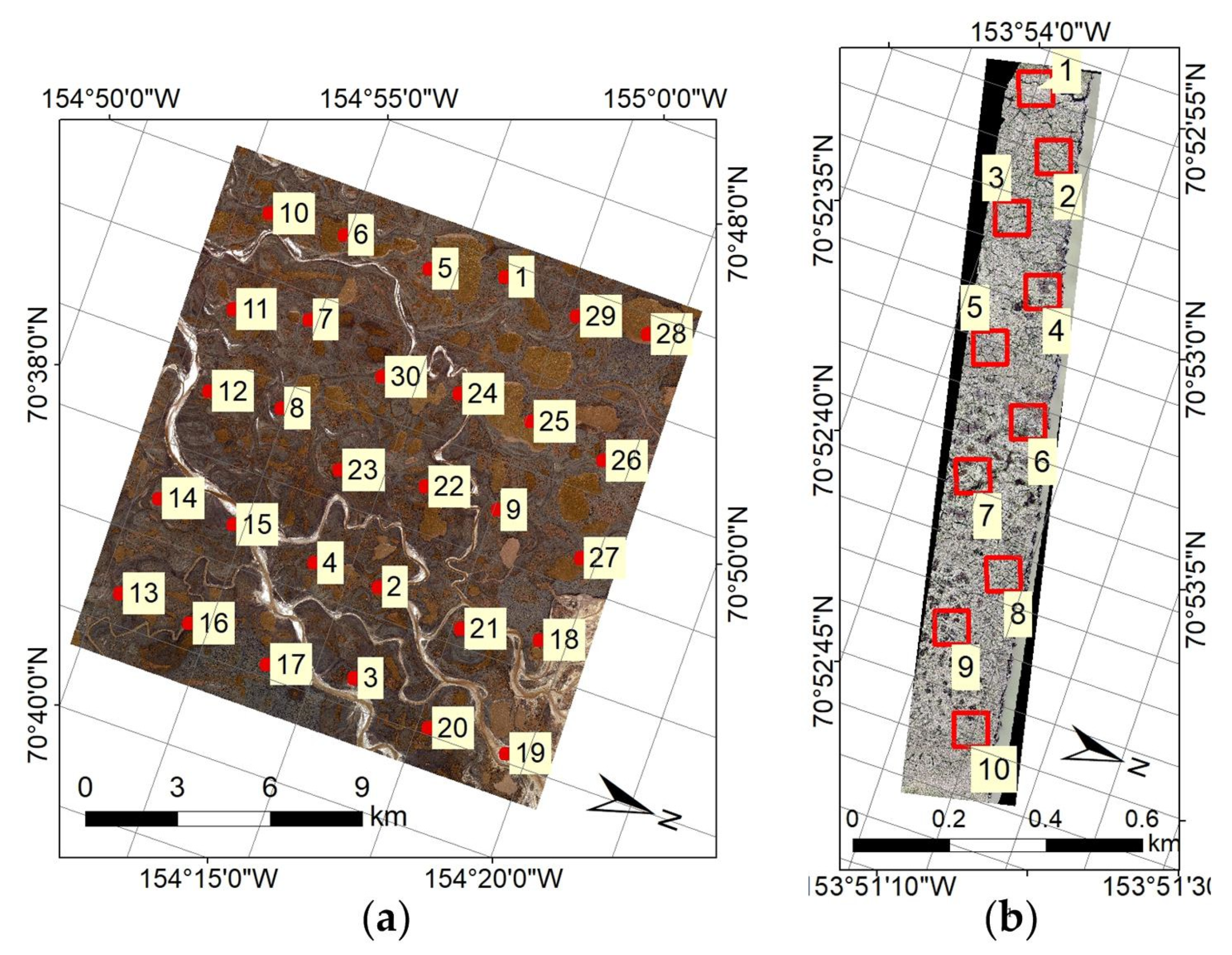
A second WorldView-2 image (image ID: 10300100468D9100, 7 July 2015, with an x- and y-resolution of 0.48 × 0.49 m, Imagery © [2015] DigitalGlobe, Inc.) represented a 272 km2 area ~50 km northeast of the 2010 annotation scene (Figure 1c and Table 1). The 2015 image was used to evaluate the trained model. Similar to the 2010 annotation scene, the 2015 image has a panchromatic band and eight multispectral band raster files, but we only used the near-infrared, green, and blue bands. The case study airborne imagery included a UAV orthophoto mosaic that was created with Pix4D Mapper version 4.3.31 using ~750 images acquired on 24 July 2018 from a DJI Phantom 4 Pro V2 UAV for a 0.32 km2 area that is located ~30 km northeast of the 2015 satellite image scene. The 1” 20 mp CMOS sensor camera on the UAV was flown at an altitude of 70 m above ground level, with front lap and side lap of 85% and 70%, respectively, and ground speed of 4.3 m/s. The resultant orthophoto mosaic had a spatial resolution of 0.02 m and three bands (red, green, and blue) (Figure 1d and Table 1). The horizontal accuracy of the orthomosaic was less than 0.08 m, as estimated from twenty-four ground control points that were established before the UAV survey. The UAV image was projected from the NAD 1983 UTM 7N to the Polar Stereographic projection system for consistency of images. Finally, the projected UAV image was resampled to 0.15 m resolution to match the resolution of training data used in the trained Mask R-CNN [17].

2.3. Annotated Data for the Mask R-CNN Model

In this study, an online accessible “VGG Image Annotator” web tool was used to conduct the object instance segmentation sampling for each cropped subset [31]. Two annotated datasets were used to train and test the Mask R-CNN model. (1) One annotated dataset (7488 IWPs) was prepared by Zhang et al. [17], which consists of 340 cropped subsets (90 × 90 m) from the Nuiqsut VHSR fixed-wing aircraft image. (2) Here we prepared an additional annotated dataset (32,367 IWPs) but from the 2010 satellite image (Figure 1b). To prepare the annotated data for the satellite image, we randomly selected 390 cropped subsets (160 × 160 m), for instance, segmentation labeling. We manually delineated all IWPs in the cropped subsets. The deep learning-based Mask R-CNN requires large amounts of training data. To keep as much training data as possible as well as enough validation and test datasets, we adopted the 8:1:1 split rule to divide the annotated data of cropped subsets randomly. Overall, the 0.15 m resolution fixed-wing aircraft aerial imagery annotated dataset has 272, 33, and 35 subsets (i.e., 6022, 668, and 798 IWPs) for training, validation, and model testing, respectively (Table 1). The 0.5 m resolution satellite imagery annotated dataset consists of 312, 39, and 39 cropped subsets (i.e., 25,498, 3470, and 3399 IWPs) as training, validation, and model testing datasets, respectively (Table 1). Low-centered ice-wedge polygons were the most common ice-wedge polygon type in the annotated images and case studies.

2.4. Annotated Data for Case Studies

We randomly chose 30 (200 × 200 m) subsets for the satellite images and 10 (70 × 70 m) subsets for the UAV images for quantitative assessments of case studies (Figure 2 and Table 1) (Note: to differentiate the testing datasets, which were prepared based on imagery data for case studies, from the model testing datasets, we named them case testing datasets). We used 200 × 200 m and 70 × 70 m block sizes to accommodate the expert-based qualitative assessments considering the workload and visual interpretation. In the preparation of case testing datasets (i.e., ground truth data) for the quantitative assessments, we manually drew boundaries of IWPs within the 40 selected subsets using the “VGG Image Annotator” web tool [31] as a reference (i.e., case testing in Table 1) dataset including 760 and 128 IWPs for the satellite and UAV images, respectively.

2.5. Experimental Design

We conducted six independent case studies (Table 2):
(C1)
We applied the Mask R-CNN model trained on VHSR fixed-wing aircraft imagery from Zhang et al. [17] to IWP mapping of a high-resolution satellite image;
(C2)
We applied the Mask R-CNN model trained only on high-resolution satellite imagery to IWP mapping of another high-resolution satellite image;
(C3)
We re-trained the model from Zhang et al. [17] with high-resolution satellite imagery and applied the model to another high-resolution satellite image;
(C4)
We applied the Mask R-CNN model trained only on high-resolution satellite imagery to IWP mapping of a 3-band UAV image;
(C5)
We applied the Mask R-CNN model trained only on VHSR fixed-wing aircraft imagery from Zhang et al. [17] to IWP mapping of the 3-band UAV image; and
(C6)
We re-trained the Mask R-CNN model already trained on high-resolution satellite imagery with VHSR fixed-wing aircraft imagery from Zhang et al. [17] and applied the model to the 3-band UAV image.
In addition to regular quantitative assessments using hold-out annotated data (i.e., modeling testing data) for the Mask R-CNN model, we conducted quantitative assessments of the detection and delineation accuracies of each case study using case testing data. Additionally, expert-based qualitative assessments of two case studies were conducted to assess the reliability of their corresponding quantitative assessments where the ground truth reference data were prepared by a non-domain expert (a non-domain expert in the Arctic). It is worth noting that we conducted the additional reliability test for two main reasons: (1) the results produced by the model can be thoroughly evaluated by a variety of domain experts; (2) it is challenging to obtain annotated datasets purely by domain experts where the data are large enough for using DL-based models.

2.6. Quantitative Assessment

We evaluated the detected and delineated IWPs that fall within the following three categories: true-positive (TP), false-positive (FP), and false-negative (FN) for detection and delineation based on 0.5 and 0.75 intersection over union (IoU) thresholds. Then we calculated the precision, recall, F1 score, and average precision (AP). The true-negative numbers are not presented because they are not required in calculating the used metrics for quantitative assessment.
The following are the equations of the precision, recall, and F1 score:
Precision = TP/(TP + FP)
Recall = TP/(TP + FN)
F1 score = (2 × Precision × Recall)/(Precision + Recall)
To be more specific, a TP detection of an IWP when the IoU threshold was 0.5 means that the IoU of the bounding box of an IWP detected by the Mask R-CNN and the bounding box of a ground truth IWP was greater than 0.5. In contrast, an FP detection of an IWP means that their bounding boxes’ IoU was less than the threshold. An FN detection of an IWP means that IoU(s) of the bounding box of a ground truth IWP was/were less than the threshold. Different than detection, delineation accuracy was evaluated according to the degree of matching between predicted and reference masks (also called polygons). A TP delineation of an IWP when the IoU threshold was 0.5 means that the IoU of the mask of an IWP predicted by the Mask R-CNN and the mask of a ground truth IWP was greater than the threshold. An FP delineation of an IWP means that their masks’ IoU was less than the threshold. An FN delineation of an IWP means that IoU(s) of the mask of a ground truth IWP was/were less than the threshold. F1 score is a weighted average of precision and recall for assessing the overall accuracy ranging from 0 (the worst) to 1 (the best). We presented the F1 score in a percentage to minimize the difference in assessment units between the quantitative and expert-based qualitative assessments. AP, which is defined as the area under the precision and recall curve, is also a metric for evaluating the performance of a method, especially when the classes are imbalanced (i.e., background and IWP in this study) [32]. A larger AP of a model means that the model had better performance, and vice versa. Finally, we calculated the precision, recall, F1 score, and AP to assess the performance of the models quantitatively.

2.7. Expert-Based Qualitative Assessment

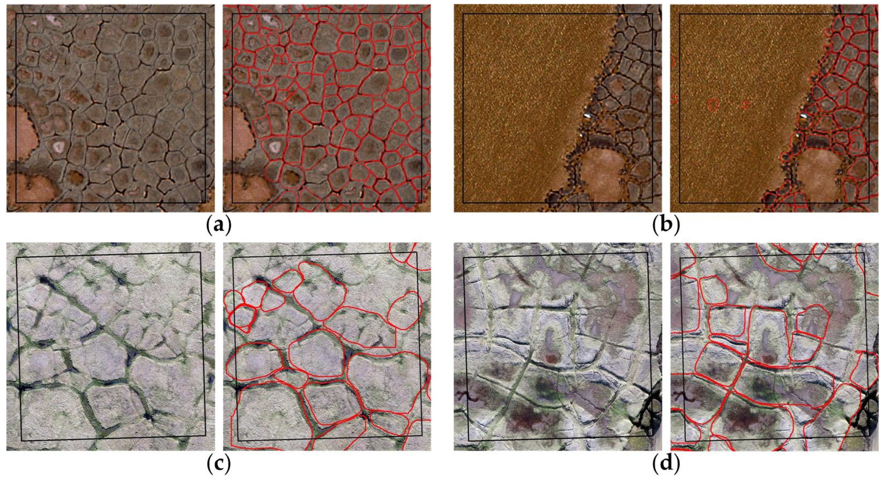
We conducted an extra expert-based qualitative assessment to examine the reliability of the quantitative assessment, which was conducted by a non-domain expert. The quantitative assessments of the C3 and C5 case studies (Table 2) were selected for this assessment. In the expert-based qualitative assessment, we re-used the selected 30 and 10 subsets used in the quantitative assessment for the satellite (Figure 3a,b) and UAV images (Figure 3c,d), respectively. The performance of Mask R-CNN for automatically mapping ice-wedge polygon objects in satellite and UAV images was assessed categorically. Six domain scientists (co-authors of this manuscript) with extensive field or remote sensing experience in the Arctic manually evaluated the accuracies of detection and delineation, and graded each subset from a range of 1 (poor) to 5 (excellent), which can be broken down into 0–20%, 20–40%, 40–60%, 60–80%, and 80–100% groupings of accuracy (i.e., poor, fair, good, very good, and excellent, correspondingly). The six experts evaluated and graded all 40 subsets for both images using the following criteria:
Detection: the estimated percentage of correct detection of IWPs by the used model within the black square box in the screenshot.
If detected:
Delineation: the estimated percentage of correct delineation of detected IWPs (i.e., among correctly detected IWPs) by the model within the black square box in the screenshot.
To maintain the objectivity of the evaluation, the location and sensor platform of the randomly selected 40 subsets for evaluation were hidden from the experts, and each expert provided their scoring independently of each other. Experts were instructed to conduct the evaluation under the following two evaluation guidelines: (1) each expert should conduct the evaluation on their own; (2) they were to spend no more than three minutes for each frame subset.

2.8. Workflow and Implementation

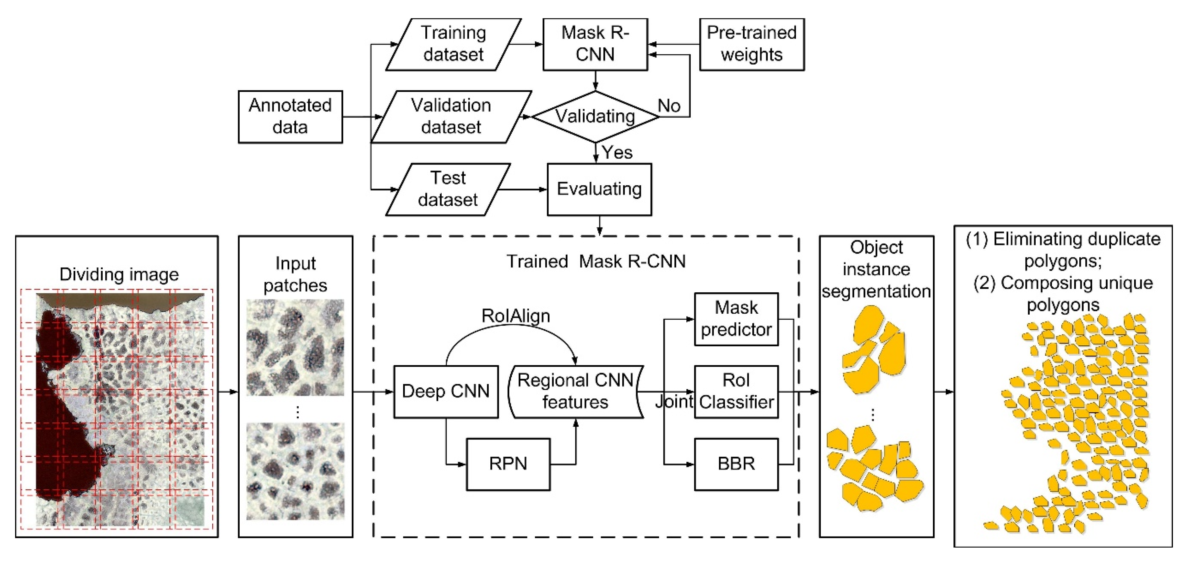
The ice-wedge polygons automated mapping workflow with the Mask R-CNN includes four components (Figure 4): (1) generating a trained model; (2) dividing input images with an overlap of 20% (160 × 160 m and 90 × 90 m block sizes were used to divide the target satellite and UAV images); (3) object instance segmentation of IWPs; (4) and eliminating duplicate IWPs and composing unique IWPs. It is worth noting that we used 160 × 160 m and 90 × 90 m block sizes to match the sizes of annotated datasets. Twenty percent overlapping (≥18 m based on the minimum block size, 90 m) is assumed to be large enough to cover each IWP because the radius of most IWPs ranges from 2.5 m to 15 m [8,33]. Duplicate IWPs can occur due to the 20% overlapping. We used a 5 m threshold of Euclidean distance between the centroids of each possible pair of IWPs to eliminate duplicate IWPs because most IWPs are wider/longer than 5 m [8,33]. Within the use of the Mask R-CNN for object instance segmentation, built-in neural networks of the Mask R-CNN are designed to extract features and then generate proposals (areas in the image which likely contain IWPs). Bounding box regressor (BBR), Mask predictor, and region of interest (RoI) classifiers are further used to delineate and classify IWPs based on the generated proposal from the previous step. We refer readers interested in the Mask R-CNN to He et al. [26] for the full description of the Mask R-CNN.
During this stage of implementation, we used an open-source package “Mask R-CNN” from Github developed by Abdulla [34]. We executed the model on an in-house GPU server at the University of Connecticut equipped with an Intel i5-7400 CPU, 16 GB RAM, and NVIDIA GeForce GTX 1070 and GTX 1080ti graphics cards. In the training process for the satellite imagery analysis, the NVIDIA GeForce GTX 1080ti graphic card was used to train the Mask R-CNN model in the package with a mini-batch size of two images, 312 steps per epoch, a learning rate of 0.001, a learning momentum of 0.9, and a weight decay of 0.0001. To implement all six case studies, we trained/re-trained six Mask R-CNN models based on the concept of transfer learning [35] (Table 2). We adopted two additional steps to minimize potential overfitting issues besides built-in regularization procedures (i.e., the augmentation of training data and early stopping). The augmentation of training data was implemented in the training data generator process for each training step, where a training dataset is randomly rotated 90° clockwise at a chance of 50%. Based on the idea of early stopping strategy, we used the hold-out annotated datasets (i.e., validation datasets) from VHSR and satellite imagery to find the convergence epoch where the validation loss value reached its lowest value by tracking and visualizing the log of the training process via the TensorBoard. Finally, we selected the best Mask R-CNN model for each case (Table 3). During the stage of prediction (i.e., mapping IWPs), the elapsed times for processing the satellite and the UAV images were around 1 h 20 min versus 0.6 min, using both NVIDIA GeForce GTX 1070 and GTX 1080ti graphics cards during each processing.

3. Case Studies and Results

3.1. Quantitative Assessment Based on Model Testing Datasets

Table 4 shows that the performance of the Mask R-CNN using the case testing data for the Mask R-CNN (798 and 3399 IWPs for the WorldView-2 satellite and fixed-wing aircraft images) when the IoU thresholds were 0.5 and 0.75, respectively. The F1 scores of detection and delineation range from 76% to 78% and from 68% to 78%. The AP detection and delineation range from 0.6 to 0.73 and from 0.66 to 0.73. The C2 and C4’s F1 scores and APs are almost as same as C3’s. Similarly, the difference between C1 and C5’s F1 scores and APs and C6’s was less than 1%. That indicates that the model did not perform better or worse in mapping IWPs even after training the model with more data of different resolutions. Compared to the change in detection accuracy as the IoU increases, the delineation accuracy did not change as the IoU increases.

3.2. Quantitative Assessment Based on Case Testing Datasets

Table 5 shows that the performance of the Mask R-CNN using the annotation data for case studies (760 and 128 IWPs for the WorldView-2 satellite and UAV images) when the IoU thresholds were 0.5 and 0.75, respectively. The F1 scores of detection and delineation ranged from 44% to 72% and from 54% to 73%. The AP detection and delineation ranged from 0.25 to 0.6 and from 0.34 to 0.58. Detection of F1 scores changed up to 16% as the IoU increased from 0.5 to 0.75. In contrast, the delineation accuracy did not change at all as the IoU increased from 0.5 to 0.75. In the following sections of the results of case studies, we only discuss the quantitative assessment results when the IoU was 0.5.

3.2.1. C1: A Mask R-CNN Model Trained Only on VHSR Fixed-Wing Aircraft Imagery Was Applied to a High-Resolution Satellite Image

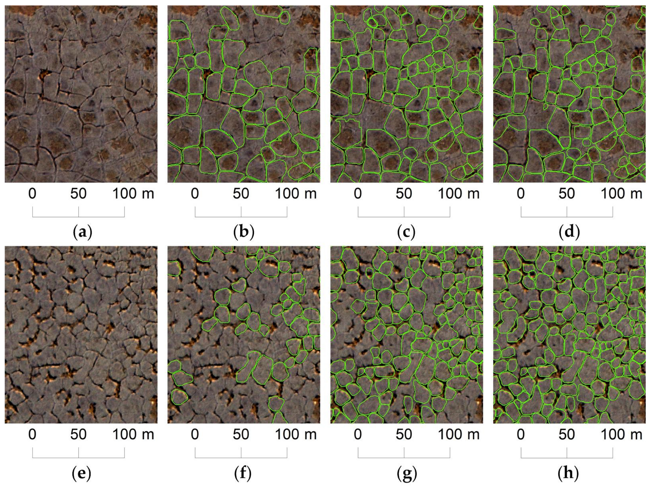
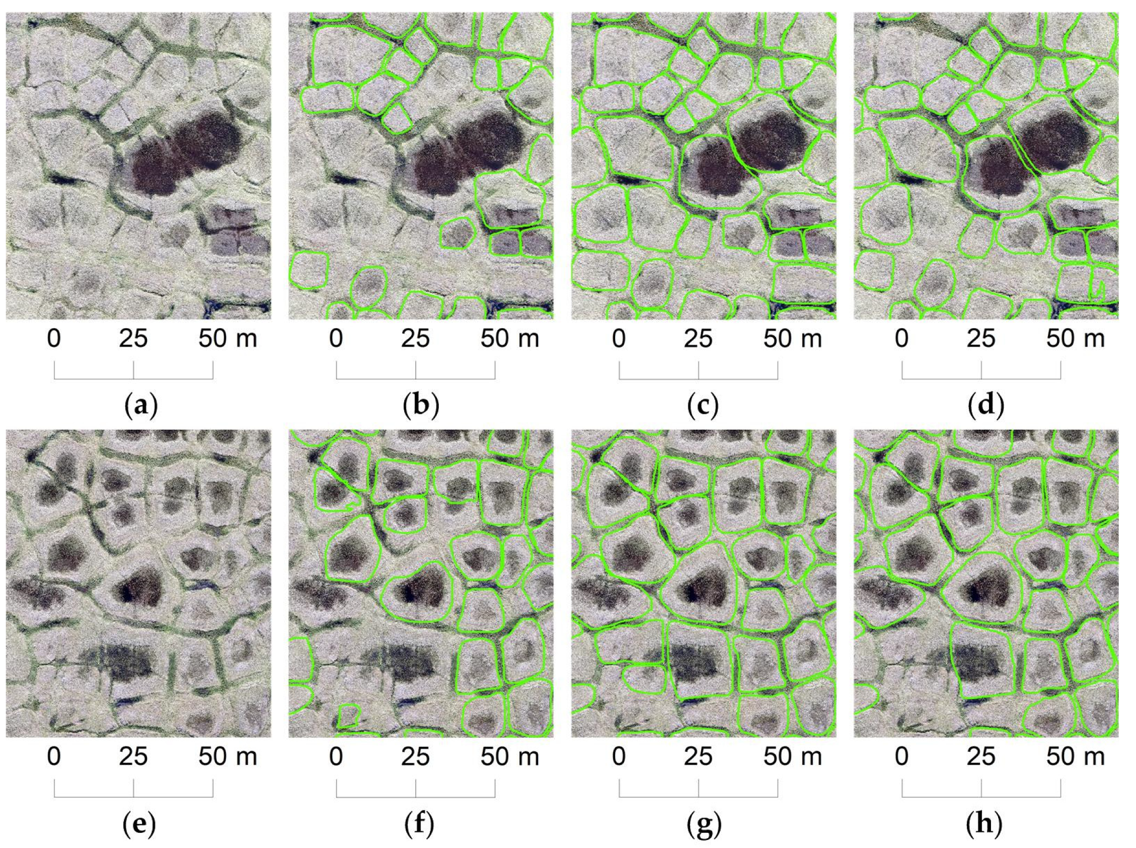
A total of 102,379 IWPs (a total area of 45.85 km2, 17% of the 272 km2 area) were mapped on the satellite imagery with both detection and delineation F1 scores of 54% when using a Mask R-CNN model trained only on VHSR fixed-wing aircraft imagery (Figure 1c and Table 5). The Mask R-CNN model presented a high precision (0.87) in terms of detection, although its F1 score was 54% (Table 5). That means most IWPs detected by the model were actual IWPs. In contrast, a 0.39 recall indicates that the model missed slightly more than half of the IWPs in the case testing datasets (Table 5). The precision of delineation was 0.87; however, the recall of delineation was 0.39. That shows that the model could correctly draw boundaries of most detected IWPs. Compared to mapping IWPs with clear boundaries (Figure 5b), the model failed in mapping disjoint/incomplete IWPs (Figure 5f). Accordingly, the model could map IWPs on coarser resolution imagery (~0.5 m resolution satellite imagery) when it was trained only on finer resolution imagery (~0.15 m resolution VHSR fixed-wing aircraft imagery).

3.2.2. C2: A Mask R-CNN Model Trained Only on High-Resolution Satellite Imagery Was Applied to Another High-Resolution Satellite Image

In the case study of applying a Mask R-CNN (trained only on a high-resolution satellite image) model to another high-resolution satellite image, the F1 scores of detection and delineation were 72% and 73% (Table 5). The precision and recall of detection and delineation were 0.68 and 0.77, and 0.69 and 0.77, respectively (Table 5). The Mask R-CNN model utilized in this case study presented better performance than the Mask R-CNN model trained only on VHSR fixed-wing aircraft imagery in detection mainly because it could correctly detect a larger number of IWPs. Similarly, both the Mask R-CNN model in C1 and in this case study were able to outline most boundaries of detected IWPs. A total of 155,296 IWPs were mapped (a total area of 37.28 km2, 14% of the 272 km2 area), which was 52,917 IWPs more than in the C1 case study. The used Mask R-CNN model was able to map many more disjoint/incomplete IWPs (Figure 5c) in addition to being able to map most IWPs with clear boundaries like the Mask R-CNN model used in the C1 case study (Figure 5g). Overall, the Mask R-CNN model that trained only on a high-resolution satellite image performs better than the Mask R-CNN model trained only on a VHSR fixed-wing aircraft image in mapping IWPs from another high-resolution satellite image.

3.2.3. C3: A Mask R-CNN Model Trained on VHSR Fixed-Wing Aircraft Imagery and Re-Trained on High-Resolution Satellite Imagery Was Applied to Another High-Resolution Satellite Image

This case study presents the results of mapping IWPs with a Mask R-CNN model which was pre-trained with VHSR fixed-wing aircraft imagery and was re-trained with high-resolution satellite imagery. A total number of 169,871 IWPs were mapped, covering a total of ~15% (a total area of 40.21 km2) of the 272 km2 area (using the total inside area of each polygon). The F1 scores of both detection and delineation were 72% (Table 5), which were very similar to the performance of the Mask R-CNN model trained only with high-resolution satellite imagery in the last case study (C2). Based on the expert evaluation, the average grades of detection and delineation were good and excellent, respectively, which means around 40–60% of IWPs in the image were correctly detected and nearly all (80–100%) detected IWPs were delineated correctly (Table 6). The result of the quantitative assessment (F1 scores of detection and delineation were 61% and 72% when the IoU was 0.75 instead of 0.5) was basically the same as the result of the expert-based quantitative assessment, which indicates that the quantitative assessment is as reliable as the one assessed by domain experts when IoU was 0.75. The enlarged subsets from the results show that the Mask R-CNN model can automatically capture most IWPs that have clearly defined rims or troughs (Figure 5d). In addition, even some “incomplete” (also known as disjoint) IWPs can be identified and mapped by the model in high-resolution satellite imagery (Figure 5h).

3.2.4. C4: A Mask R-CNN Model Trained Only on High-Resolution Satellite Imagery Was Applied to a 3-Band UAV Image

Nine hundred and fifty-two IWPs (a total area of 0.13 km2, 41% of the 0.32 km2 area) were mapped by the Mask R-CNN model trained only on high-resolution satellite imagery with the F1 scores of both detection and delineation as 61%, respectively (Table 5). Both precisions of detection and delineation (0.70 and 0.69) were greater than their recalls (0.55 and 0.54). That means, in terms of detection and delineation, around 60% IWPs detected and delineated by the model were correct, although the model missed 58 out of 128 IWPs in the case testing datasets. Figure 6f posits that most IWPs with wet centers, which appeared to be colored black, were correctly mapped. Only around half of IWPs were detected from the image if they did not have wet centers (Figure 6b). In addition, IWPs of large size (see the center part of Figure 6b and the lower-left part of Figure 6f) were not detected by the model either.

3.2.5. C5: A Mask R-CNN Model Trained Only on VHSR Fixed-Wing Aircraft Imagery Was Applied to a 3-Band UAV Image

In the case study using a UAV image (0.32 km2), a total of 931 IWPs were mapped. The coverage of IWPs in the UAV image (excluding no-data sections) was ~49%. The results from the quantitative assessment (Table 5) indicate that the F1 scores of both detection and delineation of the Mask R-CNN model were 63%. However, Table 7 shows that the average grades of detection and delineation for the UAV image were both excellent, which indicates that around 80–100% of IWPs in the UAV image were correctly detected and delineated based on the expert evaluation. There was a disagreement on the assessment between the quantitative assessment (63%) and the expert-based qualitative assessment (80–100%) regarding the delineation. The disagreements between the accuracy results of the quantitative assessment and the expert-based qualitative assessment show that the quantitative assessment was underestimated. The enlarged subsets (Figure 6) show that the Mask R-CNN model achieved visually very good performance on automatic mapping of most IWPs.

3.2.6. C6: A Mask R-CNN Model Re-Trained on High-Resolution Satellite Imagery Was Applied to a 3-Band UAV Image

In this case study, the used Mask R-CNN model was trained on high-resolution satellite imagery and VHSR fixed-wing aircraft imagery sequentially. A total of 880 IWPs (47% coverage) with a total area of 0.15 km2 were detected and delineated. The F1 scores of both detection (70%) and delineation (68%), when more training data were used to train the model, were around 7% better as compared to the last two case studies (C4 and C5), correspondingly (Table 5). Particularly, the recall of detection of this Mask R-CNN model was 0.68 compared to 0.55 in the C4 and C5 case studies (Table 5). Figure 6d,h show that the selected enlarged subsets posit that the model could still correctly map most IWPs. However, the excellent results presented in Figure 6d,h might be coincident because only four randomly selected enlarged subsets were presented compared to ten that were used for the quantitative assessment.

4. Discussion

4.1. Effect of Spatial Resolution of Training Data on Mask R-CNN Performance

Our results show that the Mask R-CNN model performed satisfactorily in identifying IWPs (54–72% F1 scores for satellite imagery and 61–70% F1 scores for the UAV photo) and in delineating the identified IWPs (54–73% F1 scores for satellite imagery and 61–68% F1 scores for the UAV photo). The model could still achieve an F1 score of 54% for both detection and delineation in mapping IWPs from satellite imagery (0.5 m) despite the fact that the model was trained only on finer resolution imagery (0.15 m). Our results (C2: the model trained only on high-resolution satellite imagery versus C3: re-trained the model from Zhang et al. [17] with high-resolution satellite imagery) also indicate that more training data with a different resolution than the target imagery do not necessarily result in a better performance of a Mask R-CNN model. For instance, in the C3 case study, F1 scores of detection and delineation were 72% (Table 5). They were almost the same as the corresponding F1 scores (72% and 73%) in the C2 case study (Table 5). However, more training data with different resolutions resulted in an improved performance of the model based on the results of the C5 and C6 case studies (C5: the model trained only on VHSR fixed-wing aircraft imagery from Zhang et al. [17] versus C6: re-trained the Mask R-CNN model already trained on high-resolution satellite imagery with VHSR fixed-wing aircraft imagery from Zhang et al. [17]). The F1 scores for detection and delineation declined from 63% and 63% to 70% and 68%, respectively (Table 5).
Our results (APs) also indicate that the effectiveness of the Mask R-CNN model in detecting IWPs was generally better with the UAV imagery than with the satellite imagery, which in this case, may be partially explained by the difference in spatial resolution between the training dataset image and the target satellite image. To be specific, in the case studies (i.e., C2 and C3) of sub-meter resolution satellite imagery, the training dataset was prepared based on a satellite image with an x- and y-resolution of 0.8 × 0.66 m but the target satellite image for the case study had 0.48 × 0.49 m for x- and y-resolution. Overall, the model consistently underestimated IWP coverage no matter how fine the spatial resolution of the imagery was, but the underestimation issue was slightly worse at the satellite image with the ~0.5 m resolution (54–72% F1 scores for detection) compared to the UAV image with the 0.15 m resolution (61–70% F1 scores for detection) (Table 5).

4.2. Effect of Used Spectral Bands of Training Data on Mask R-CNN Performance

Our results show that spectral bands in the training data had a limited effect on the Mask R-CNN model performance. The C4, C5, and C6 case studies show that the training model for the 0.15 m fixed-wing aircraft and 0.6~0.8 m satellite imagery included near-infrared, green, and blue bands, while the UAV image had red, green, and blue bands. Even so, based on the quantitative assessment, around 61–70% of IWPs were still correctly detected, and around 61–68% of the detected IWPs were correctly delineated from the UAV image (Table 5). The results highlight the robustness of a CNN-based deep learning approach for mapping IWPs, which is based upon pattern recognition of high-level feature representations (e.g., edges, curves, and shapes of objects) rather than low-level features (e.g., lines, dots, and colors). Therefore, the Mask R-CNN model can be considered a highly flexible IWP mapping method handling high-resolution RS images acquired across airborne platforms and sensors.

4.3. Limitations of the Mask R-CNN Model

From the perspective of the performance of mapping IWPs, the Mask R-CNN model can map most IWPs with distinct rims or troughs, but it has difficulty handling “incomplete” or faintly evident IWPs (Figure 5b,f and Figure 6b,f). It is to be expected that the Mask R-CNN model failed to capture such IWPs because the approach was an instance segmentation model that identified separable individual object outlines (disjoint/incomplete IWPs are not separable individual objects (Figure 5b,f and Figure 6b,f). A multi-level hybrid segmentation model that combines semantic and instance segmentation may be able to map both complete and disjoint/incomplete IWPs.
It is important to mention that comprehensive comparison studies on instance segmentation methods are necessary to assess which option is the most effective in mapping IWPs. The machine learning field changes at a rapid pace. New machine learning models come out frequently, and most of them do not become quickly accessible to the public. A few instance/panoptic segmentation models, such as Path Aggregation Network [36], Mask Scoring R-CNN [37], Cascade R-CNN [38], and Hybrid Task Cascade [39], have been proven to marginally outperform the Mask R-CNN since 2017 from the perspective of mean AP [27]. The results are also a conservative estimate of ice-wedge coverage as ice-wedges can be abundant in some types of permafrost terrain without them being evident from surface microtopography. Thus, the lack of IWPs being mapped (no matter how sophisticated the model) does not necessarily mean that subsurface ice wedges are absent.

4.4. Limitations of the Annotation Data

The quality of annotation data affects the accuracy of IWP mapping. The Mask R-CNN model is similar to other DL models in that the model is as biased as the human that is preparing the model training dataset. Here, one feedback from the expert evaluation assessment was that an occasional non-existing polygon was mistakenly detected by the model. The effort could be further improved if the training dataset (and not just the results) had been prepared, or at least reviewed and evaluated, by experts prior to training the DL model. Additionally, similar to other DL models, the Mask R-CNN model is a data-driven model that requires a large number of quality training datasets to achieve outstanding performance. A small number of training datasets from imagery acquired from a certain period, location, terrain, and so forth, could result in a poor generalization of a DL model. However, given currently limited manpower, only a comparably limited amount (number and location) of training datasets based on satellite and fixed-wing aircraft aerial imagery (25,498 and 6022 manually delineated ice-wedge polygons, respectively) were prepared and used, so the full potential of the Mask R-CNN approach was not truly explored. Therefore, an increased number of quality training datasets that represent the variability in the region (e.g., images acquired from various seasons, regions, terrains, etc.) is expected to improve the performance further and, therefore, benefit larger-scale regional applications.

5. Conclusions

We examined the transferability of a deep learning Mask R-CNN model to map ice-wedge polygons with respect to the spatial resolution and spectral bands of input imagery. We conclude that the Mask R-CNN model is an effective but conservative method for automated mapping of IWPs with sub-meter resolution satellite or UAV imagery, achieving better performance with finer resolution imagery, regardless of spectral bands. The increasing availability of sub-meter resolution commercial satellite imagery and drone photogrammetry provides great opportunities for Arctic researchers to document, analyze, and understand fine-scale permafrost processes that occur across the local to pan-Arctic domains in response to climate warming or other disturbances. The mapping models will continue to improve, while the increasing volumes of data will demand even more efficient mapping workflows and the development of end-user friendly post-processing tools to make the final big data products accessible and discoverable.

Author Contributions

W.Z. contributed to the design and conceived the study, collected the data, performed the experiments, and wrote and revised the manuscript. A.K.L. and M.K. were involved in study design from the perspective of Arctic Science and contributed to the manuscript writing and revision. B.M.J., H.E.E., M.T.J., and K.K. contributed to the results assessment and manuscript revision. All authors have read and agreed to the published version of the manuscript.

Funding

This work was supported by the U.S. National Science Foundation’s Office of Polar Programs [grant No. 1720875, 1722572, and 1721030] and Office of Integrative Activities [grant No. 1929170]. Geospatial support for this work was provided by the Polar Geospatial Center under NSF-OPP awards [No. 1043681 and 1559691].

Acknowledgments

The authors would like to thank the Department of Geography at the University of Connecticut for providing GPU devices and Waleed Abdulla of Mask R-CNN for sharing codes on Github (https://github.com/matterport/Mask_RCNN). We also thank Krista Rogers for checking the English of this manuscript, Richard Buzard for providing insight on conducting well-constrained UAV survey data collection, and Chandi Witharana for postdoctoral mentoring. Satellite imagery © [2015] DigitalGlobe, Inc.

Conflicts of Interest

The authors declare no conflict of interest. The founding sponsors had no role in the design of the study; in the collection, analyses, or interpretation of data; in the writing of the manuscript, and in the decision to publish the results.

References

  1. Muller, S.W. Permafrost or Permanently Frozen Ground and Related Engineering Problems; J. W. Edwards Inc.: Ann Arbor, MI, USA, 1947. [Google Scholar]
  2. van Everdingen, R.O. Multi-Language Glossary of Permafrost and Related Ground-Ice; Arctic Institute of North America in University of Calgary: Calgary, AL, Canada, 1998. [Google Scholar]
  3. Jorgenson, M.T.; Kanevskiy, M.; Shur, Y.; Moskalenko, N.; Brown, D.R.N.; Wickland, K.; Striegl, R.; Koch, J. Role of ground ice dynamics and ecological feedbacks in recent ice wedge degradation and stabilization. J. Geophys. Res. Earth Surf. 2015, 120, 2280–2297. [Google Scholar] [CrossRef]
  4. Leffingwell, E.D.K. Ground-Ice Wedges: The Dominant Form of Ground-Ice on the North Coast of Alaska. J. Geol. 1915, 23, 635–654. [Google Scholar] [CrossRef]
  5. Lachenbruch, A.H. Mechanics of Thermal Contraction Cracks and Ice-Wedge Polygons in Permafrost; Geological Society of America: Boulder, CO, USA, 1962; Volume 70. [Google Scholar]
  6. Dostovalov, B.N. Polygonal Systems of Ice Wedges and Conditions of Their Development. In Proceedings of the Permafrost International Conference, Lafayette, IN, USA, 11–15 November 1963. [Google Scholar]
  7. Mackay, J.R. The World of Underground Ice. Ann. Assoc. Am. Geogr. 1972, 62, 1–22. [Google Scholar] [CrossRef]
  8. Kanevskiy, M.Z.; Shur, Y.; Jorgenson, M.T.; Ping, C.-L.; Michaelson, G.J.; Fortier, D.; Stephani, E.; Dillon, M.; Tumskoy, V. Ground ice in the upper permafrost of the Beaufort Sea coast of Alaska. Cold Reg. Sci. Technol. 2013, 85, 56–70. [Google Scholar] [CrossRef]
  9. Jorgenson, M.T.; Shur, Y.L.; Pullman, E.R. Abrupt increase in permafrost degradation in Arctic Alaska. Geophys. Res. Lett. 2006, 33. [Google Scholar] [CrossRef]
  10. Liljedahl, A.K.; Boike, J.; Daanen, R.P.; Fedorov, A.N.; Frost, G.V.; Grosse, G.; Hinzman, L.D.; Iijma, Y.; Jorgenson, J.C.; Matveyeva, N.; et al. Pan-Arctic ice-wedge degradation in warming permafrost and its influence on tundra hydrology. Nat. Geosci. 2016, 9, 312–318. [Google Scholar] [CrossRef]
  11. Fraser, R.H.; Kokelj, S.V.; Lantz, T.C.; McFarlane-Winchester, M.; Olthof, I.; Lacelle, D. Climate Sensitivity of High Arctic Permafrost Terrain Demonstrated by Widespread Ice-Wedge Thermokarst on Banks Island. Remote Sens. 2018, 10, 954. [Google Scholar] [CrossRef] [Green Version]
  12. Frost, G.V.; Epstein, H.E.; Walker, D.A.; Matyshak, G.; Ermokhina, K. Seasonal and Long-Term Changes to Active-Layer Temperatures after Tall Shrubland Expansion and Succession in Arctic Tundra. Ecosystems 2018, 21, 507–520. [Google Scholar] [CrossRef]
  13. Jones, B.M.; Grosse, G.; Arp, C.D.; Miller, E.; Liu, L.; Hayes, D.J.; Larsen, C.F. Recent Arctic tundra fire initiates widespread thermokarst development. Sci. Rep. 2015, 5, 15865. [Google Scholar] [CrossRef] [Green Version]
  14. Raynolds, M.K.; Walker, D.A.; Ambrosius, K.J.; Brown, J.; Everett, K.R.; Kanevskiy, M.; Kofinas, G.P.; Romanovsky, V.E.; Shur, Y.; Webber, P.J. Cumulative geoecological effects of 62 years of infrastructure and climate change in ice-rich permafrost landscapes, Prudhoe Bay Oilfield, Alaska. Glob. Chang. Biol. 2014, 20, 1211–1224. [Google Scholar] [CrossRef]
  15. Jorgenson, M.T.; Shur, Y.L.; Osterkamp, T.E. Thermokarst in Alaska. In Proceedings of the Ninth International Conference on Permafrost, Fairbanks, AK, USA, 29 June–3 July 2008; University of Alaska-Fairbanks: Fairbanks, AK, USA; pp. 121–122. Available online: https://www.researchgate.net/profile/Sergey_Marchenko3/publication/334524021_Permafrost_Characteristics_of_Alaska_Map/links/5d2f7672a6fdcc2462e86fae/Permafrost-Characteristics-of-Alaska-Map.pdf (accessed on 1 May 2019).
  16. Gorelick, N.; Hancher, M.; Dixon, M.; Ilyushchenko, S.; Thau, D.; Moore, R. Google Earth Engine: Planetary-scale geospatial analysis for everyone. Remote Sens. Environ. 2017, 202, 18–27. [Google Scholar] [CrossRef]
  17. Zhang, W.; Witharana, C.; Liljedahl, A.K.; Kanevskiy, M. Deep Convolutional Neural Networks for Automated Characterization of Arctic Ice-Wedge Polygons in Very High Spatial Resolution Aerial Imagery. Remote Sens. 2018, 10, 1487. [Google Scholar] [CrossRef] [Green Version]
  18. Abolt, C.J.; Young, M.H.; Atchley, A.L.; Wilson, C.J. Brief communication: Rapid machine-learning-based extraction and measurement of ice wedge polygons in high-resolution digital elevation models. Cryosphere 2019, 13, 237–245. [Google Scholar] [CrossRef] [Green Version]
  19. Lara, M.J.; Chipman, M.L.; Hu, F.S. Automated detection of thermoerosion in permafrost ecosystems using temporally dense Landsat image stacks. Remote Sens. Environ. 2019, 221, 462–473. [Google Scholar] [CrossRef]
  20. Cooley, S.W.; Smith, L.C.; Ryan, J.C.; Pitcher, L.H.; Pavelsky, T.M. Arctic-Boreal Lake Dynamics Revealed Using CubeSat Imagery. Geophys. Res. Lett. 2019, 46, 2111–2120. [Google Scholar] [CrossRef]
  21. Nitze, I.; Grosse, G.; Jones, B.M.; Arp, C.D.; Ulrich, M.; Fedorov, A.; Veremeeva, A. Landsat-Based Trend Analysis of Lake Dynamics across Northern Permafrost Regions. Remote Sens. 2017, 9, 640. [Google Scholar] [CrossRef] [Green Version]
  22. Nitze, I.; Grosse, G.; Jones, B.M.; Romanovsky, V.E.; Boike, J. Remote sensing quantifies widespread abundance of permafrost region disturbances across the Arctic and Subarctic. Nat. Commun. 2018, 9, 5423–5434. [Google Scholar] [CrossRef]
  23. LeCun, Y.; Bengio, Y.; Hinton, G. Deep learning. Nature 2015, 521, 436–444. [Google Scholar] [CrossRef]
  24. Diao, W.; Sun, X.; Dou, F.; Yan, M.; Wang, H.; Fu, K. Object recognition in remote sensing images using sparse deep belief networks. Remote Sens. Lett. 2015, 6, 745–754. [Google Scholar] [CrossRef]
  25. Guan, H.; Yu, Y.; Ji, Z.; Li, J.; Zhang, Q. Deep learning-based tree classification using mobile LiDAR data. Remote Sens. Lett. 2015, 6, 864–873. [Google Scholar] [CrossRef]
  26. He, K.; Gkioxari, G.; Dollár, P.; Girshick, R. Mask r-cnn. In Proceedings of the 2017 IEEE International Conference on Computer Vision (ICCV), Venice, Italy, 22–29 October 2017; IEEE: Piscataway, NJ, USA, 2017; pp. 2961–2969. [Google Scholar] [CrossRef]
  27. Bolya, D.; Zhou, C.; Xiao, F.; Lee, Y.J. YOLACT++: Better Real-time Instance Segmentation. arXiv 2019, arXiv:1912.06218. Available online: https://arxiv.org/abs/1912.06218 (accessed on 1 March 2020).
  28. Lin, T.-Y.; Maire, M.; Belongie, S.; Bourdev, L.; Girshick, R.; Hays, J.; Perona, P.; Ramanan, D.; Zitnick, C.L.; Dollár, P. Microsoft COCO: Common Objects in Context. In Computer Vision—ECCV 2014; Fleet, D., Pajdla, T., Schiele, B., Tuytelaars, T., Eds.; Springer: Cham, Switzerland, 2014; Volume 8693, pp. 740–755. ISBN 978-3-319-10601-4. [Google Scholar] [CrossRef] [Green Version]
  29. Dai, J.; He, K.; Sun, J. Instance-Aware Semantic Segmentation via Multi-Task Network Cascades. In Proceedings of the IEEE Conference on Computer Vision and Pattern Recognition (CVPR), Las Vegas, NV, USA, 26 June–1 July 2016; IEEE: Piscataway, NJ, USA, 2016; pp. 3150–3158. Available online: https://www.cv-foundation.org/openaccess/content_cvpr_2016/html/Dai_Instance-Aware_Semantic_Segmentation_CVPR_2016_paper.html (accessed on 1 March 2020).
  30. Li, Y.; Qi, H.; Dai, J.; Ji, X.; Wei, Y. Fully Convolutional Instance-Aware Semantic Segmentation. In Proceedings of the IEEE Conference on Computer Vision and Pattern Recognition (CVPR), Honolulu, HI, USA, 21–26 July 2017; IEEE: Piscataway, NJ, USA, 2017; pp. 2359–2367. Available online: http://openaccess.thecvf.com/content_cvpr_2017/html/Li_Fully_Convolutional_Instance-Aware_CVPR_2017_paper.html (accessed on 5 March 2020).
  31. Dutta, A.; Zisserman, A. The VIA Annotation Software for Images, Audio and Video. In Proceedings of the 27th ACM International Conference on Multimedia, Nice, France, 21–25 October 2019; ACM: New York, NY, USA, 2019; pp. 2276–2279. [Google Scholar] [CrossRef] [Green Version]
  32. Huang, L.; Luo, J.; Lin, Z.; Niu, F.; Liu, L. Using deep learning to map retrogressive thaw slumps in the Beiluhe region (Tibetan Plateau) from CubeSat images. Remote Sens. Environ. 2020, 237, 111534. [Google Scholar] [CrossRef]
  33. Chen, Z.; Pasher, J.; Duffe, J.; Behnamian, A. Mapping Arctic Coastal Ecosystems with High Resolution Optical Satellite Imagery Using a Hybrid Classification Approach. Can. J. Remote Sens. 2017, 43, 513–527. [Google Scholar] [CrossRef]
  34. Abdulla, W. Mask r-cnn for Object Detection and Instance Segmentation on Keras and Tensorflow. GitHub Repos. 2017. Available online: https://github.com/matterport/Mask_RCNN (accessed on 1 November 2018).
  35. Pan, S.J.; Yang, Q. A Survey on Transfer Learning. IEEE Trans. Knowl. Data Eng. 2010, 22, 1345–1359. [Google Scholar] [CrossRef]
  36. Liu, S.; Qi, L.; Qin, H.; Shi, J.; Jia, J. Path Aggregation Network for Instance Segmentation. In Proceedings of the IEEE Conference on Computer Vision and Pattern Recognition (CVPR), Salt Lake City, UT, USA, 18–22 June 2018; IEEE: Piscataway, NJ, USA, 2018; pp. 8759–8768. Available online: http://openaccess.thecvf.com/content_cvpr_2018/html/Liu_Path_Aggregation_Network_CVPR_2018_paper.html (accessed on 5 March 2020).
  37. Huang, Z.; Huang, L.; Gong, Y.; Huang, C.; Wang, X. Mask Scoring R-CNN. In Proceedings of the IEEE Conference on Computer Vision and Pattern Recognition (CVPR), Long Beach, CA, USA, 16–20 June 2019; IEEE: Piscataway, NJ, USA, 2019; pp. 6409–6418. Available online: http://openaccess.thecvf.com/content_CVPR_2019/html/Huang_Mask_Scoring_R-CNN_CVPR_2019_paper.html (accessed on 5 March 2020).
  38. Cai, Z.; Vasconcelos, N. Cascade R-CNN: High Quality Object Detection and Instance Segmentation. IEEE Trans. Pattern Anal. Mach. Intell. 2019. [Google Scholar] [CrossRef] [Green Version]
  39. Chen, K.; Ouyang, W.; Loy, C.C.; Lin, D.; Pang, J.; Wang, J.; Xiong, Y.; Li, X.; Sun, S.; Feng, W.; et al. Hybrid Task Cascade for Instance Segmentation. In Proceedings of the IEEE Conference on Computer Vision and Pattern Recognition (CVPR), Long Beach, CA, USA, 16–20 June 2019; IEEE: Piscataway, NJ, USA, 2019; pp. 4969–4978. Available online: http://openaccess.thecvf.com/content_CVPR_2019/html/Chen_Hybrid_Task_Cascade_for_Instance_Segmentation_CVPR_2019_paper.html (accessed on 5 March 2020).
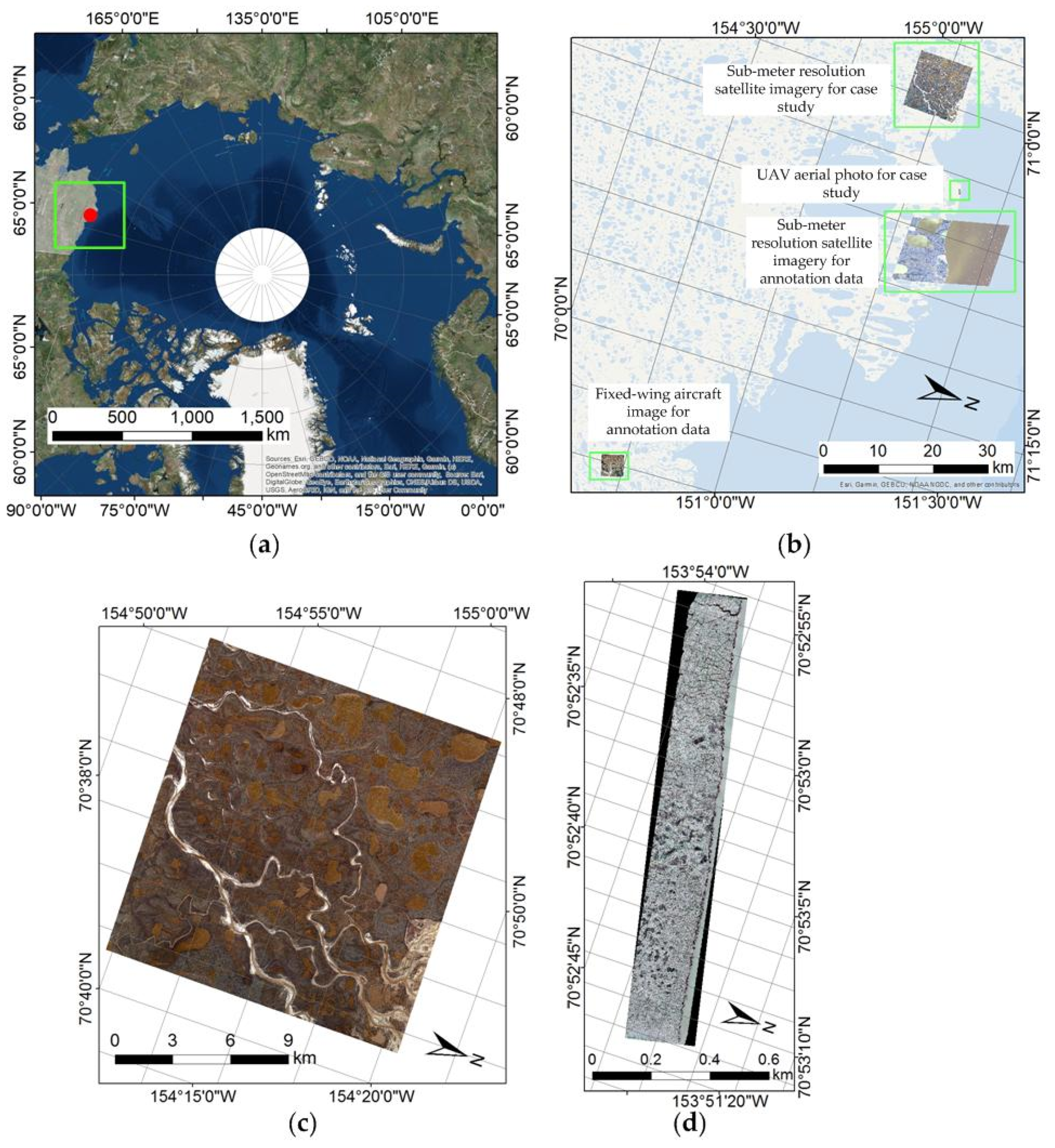
Figure 1. Both target images are located near Drew Point, Alaska (see red dot) (a). Locations of all images used in this study (see green boxes) are presented in (b). The images used in the case studies included (c) the fused WorldView-2 (Imagery © [2015] DigitalGlobe, Inc.), and (d) the UAV images.
Remotesensing 12 01085 g001
Figure 2. Locations of performance assessment of the thirty (a) and ten (b) subsets (red squares) from the satellite and UAV images.
Remotesensing 12 01085 g002
Figure 3. Examples of the ice-wedge polygons (IWP) detection and delineation results for expert-based qualitative assessment; (a,b): results of the IWP detection and delineation using the sub-meter resolution satellite image (Imagery © [2015] DigitalGlobe, Inc.); (c,d): results of the IWP detection and delineation using the unmanned aerial vehicle (UAV) image.
Remotesensing 12 01085 g003
Figure 4. Ice-wedge polygon automated mapping workflow with the implementation of the Mask Region-Based Convolutional Neural Network (R-CNN). In this figure, RoI stands for region of interest; CNN stands for convolutional neural network; RPN stands for region proposal network; BBR stands for bounding box regressor.
Remotesensing 12 01085 g004
Figure 5. Examples of results of the IWP detection and delineation using the high-resolution satellite image. Enlarged portions of the satellite image (a,e); mapped IWPs from (a) with green boundaries of IWPs delineated by the Mask R-CNN models used in the C1, C2, and C3 case studies (bd); mapped IWPs from (e) with green boundaries of IWPs delineated by the Mask R-CNN models used in the C1, C2, and C3 case studies (fh). Imagery © [2015] DigitalGlobe, Inc.
Remotesensing 12 01085 g005
Figure 6. Examples of results of the IWP detection and delineation using the UAV image. Enlarged portions of the UAV image (a,e); mapped IWPs from (a) with green boundaries of IWPs delineated by the Mask R-CNN models used in the C4, C5, and C6 case studies (bd); mapped IWPs from (e) with green boundaries of IWPs delineated by the Mask R-CNN models used in the C4, C5, and C6 case studies (fh). Imagery © [2015] DigitalGlobe, Inc.
Remotesensing 12 01085 g006
Table 1. Description of used datasets.
CategorySensor PlatformImage IDAcquired DateSpatial ResolutionUsed Spectral BandsArea (sq km)PurposeNumber of Annotated IWPs
Imagery Data for AnnotationFixed-wing Aircraftn/a09/20130.15 × 0.15 mnear-infrared, green, and blue 42Training6022
Validation668
Model Testing798
WorldView-2 Satellite10300100065AFE0007/29/20100.8 × 0.66 mnear-infrared, green, and blue 535Training25,498
Validation3470
Model Testing3399
Imagery Data for Case StudiesWorldView-2 Satellite10300100468D910007/07/20150.48 × 0.49 mnear-infrared, green, and blue 272Case Testing760
DJI Phantom 4 UAV n/a07/24/20180.02 × 0.02 mred, green, and blue0.32Case Testing128
Table 2. Description of case studies and their corresponding research questions.
Case StudyPretrained Weight DatasetRetrained Weights DatasetTarget ImageryAddressing Questions
C1 VHSR fixed-wing aircraft imageryWorldview2 imageryQ1, Q2
C2 Worldview2 imageryQ1, Q3
C3VHSR fixed-wing aircraft imageryWorldview2 imageryQ1, Q3
C4 Worldview2 imageryUAV photoQ1, Q2
C5 VHSR fixed-wing aircraft imageryQ1, Q2
C6Worldview2 imageryVHSR fixed-wing aircraft imageryQ1, Q3
Note: all models used the COCO dataset as the base weights [28].
Table 3. The number of epochs in re-training processes until the validation losses converge for obtaining the best Mask Region-Based Convolutional Neural Network (R-CNN) models correspondingly.
Case StudyThe Number of Epochs in Pre-Training ProcessesThe Number of Epochs in Re-Training Processes
C1None8
C2None70
C3855
C4None70
C5None8
C6703
Table 4. Comparison of results of different processing combinations of quantitative assessment based on model testing datasets.
Case StudyCategoryIoUTPFPFNPrecisionRecallF1AP
C1 and C5Detection0.55961322020.820.7578%0.73
0.755192092790.710.6568%0.60
Delineation0.55911372070.810.7477%0.72
0.755911372070.810.7477%0.72
C2 and C4Detection0.521517712480.970.6376%0.66
0.75206016813390.920.6173%0.63
Delineation0.521517712480.970.6376%0.66
0.7521517712480.970.6376%0.66
C3Detection0.521318212680.960.6376%0.66
0.75200620713930.910.5971%0.61
Delineation0.521308312690.960.6376%0.66
0.7521308312690.960.6376%0.66
C6Detection0.56181601800.790.7778%0.73
0.755342442640.690.6768%0.61
Delineation0.56171611810.790.7778%0.73
0.756171611810.790.7778%0.73
TP: true-positive; FP: false-positive; FN: false-negative; IoU: intersection over union; AP: average precision.
Table 5. Comparison of results of different processing combinations of quantitative assessment based on case testing datasets.
Case StudyCategoryIoUTPFPFNPrecisionRecallF1AP
C1Detection0.5300434600.870.3954%0.34
0.752431005170.710.3244%0.25
Delineation0.5298454620.870.3954%0.34
0.75298454620.870.3954%0.34
C2Detection0.55832691770.680.7772%0.54
0.754803722800.560.6360%0.41
Delineation0.55872651730.690.7773%0.55
0.755872651730.690.7773%0.55
C3Detection0.56023071580.660.7972%0.54
0.755074022530.560.6761%0.42
Delineation0.56013081590.660.7972%0.54
0.756013081590.660.7972%0.54
C4Detection0.57030580.700.5561%0.45
0.755149770.510.4045%0.26
Delineation0.56931590.690.5461%0.44
0.756931590.690.5461%0.44
C5Detection0.57127570.720.5563%0.49
0.756137670.620.4854%0.40
Delineation0.57127570.720.5563%0.49
0.757127570.720.5563%0.49
C6Detection0.58734410.720.6870%0.60
0.757249560.600.5658%0.48
Delineation0.58536430.700.6668%0.58
0.758536430.700.6668%0.58
TP: true-positive; FP: false-positive; FN: false-negative; IoU: intersection over union; AP: average precision.
Table 6. Results from the expert-based qualitative assessment on a Mask R-CNN model (re-trained on high-resolution satellite imagery) in mapping ice-wedge polygons from ~0.5 m resolution satellite imagery, Arctic Coastal Plain, northern Alaska.
Average Grades of DetectionAverage Grades of Delineation
Expert 13.74.6
Expert 23.54.3
Expert 32.94.6
Expert 43.14.2
Expert 534.6
Expert 63.84.4
Average grades3.3 (good)4.5 (excellent)
Table 7. Results from the expert-based qualitative assessment on a Mask R-CNN model (trained only on VHSR fixed-wing aircraft imagery) in mapping ice-wedge polygons from a 0.15 m resolution UAV image, Arctic Coastal Plain, northern Alaska.
Average Grades of DetectionAverage Grades of Delineation
Expert 144.5
Expert 24.33
Expert 34.14.7
Expert 44.74.4
Expert 544
Expert 64.34.7
Average grades4.2 (excellent)4.2 (excellent)