Article

Impact of Molecular Spectroscopy on Carbon Monoxide Abundances from SCIAMACHY

DLR—German Aerospace Center, Remote Sensing Technology Institute, 82234 Oberpfaffenhofen, Germany
*
Author to whom correspondence should be addressed.
Remote Sens. 2020, 12(7), 1084; https://doi.org/10.3390/rs12071084
Submission received: 13 February 2020 / Revised: 23 March 2020 / Accepted: 25 March 2020 / Published: 27 March 2020

Abstract

:
High-quality observations have indicated the need for improved molecular spectroscopy for accurate atmospheric characterization. Line data provided by the new SEOM-IAS (Scientific Exploitation of Operational Missions—Improved Atmospheric Spectroscopy) database in the shortwave infrared (SWIR) region were used to retrieve CO total vertical columns from a selected set of nadir SCIAMACHY (SCanning Imaging Absorption SpectroMeter for Atmospheric CHartographY) observations. In order to assess the quality of the retrieval results, differences in the spectral fitting residuals with respect to the HITRAN 2016 (High-resolution TRANsmission molecular absorption) and GEISA 2015 (Gestion et Etude des Informations Spectroscopiques Atmosphériques) line lists were quantified and column-averaged dry-air CO mole fractions were compared to NDACC (Network for the Detection of Atmospheric Composition Change) and TCCON (Total Carbon Column Observing Network) ground-based measurements. In general, it was found that using SEOM-IAS line data with corresponding line models improve the spectral quality of the retrieval (smaller residuals) and increase the fitted CO columns, thereby reducing the bias to both ground-based networks.

Graphical Abstract

1. Introduction

Remote sensing is an important asset in monitoring the state of Earth’s atmosphere. Only space-borne instruments are providing continuous global coverage and are now invaluable for long-term atmospheric characterization and measurements in the context of climate change, stratospheric ozone depletion, and regional air quality studies. Low Earth-orbiting sensors are complemented by numerous balloon- or airborne sensors as well as ground-based instrumentation that is important for the validation of satellite observations as well as for dedicated studies. In all cases a rigorous assessment of the quality of the remote-sensing products is essential and necessary.
Quantification of atmospheric state variables from remote-sensing instruments constitutes an inverse problem that is usually solved by the iterative solution of an optimization problem with repeated calls to a forward model. Among the numerous parameters required by the forward model (essentially comprising atmospheric radiative transfer and an instrument model) and the inversion algorithm, the spectroscopic data characterizing the atmospheric species play a central role [1,2,3,4,5,6,7,8]. More specifically, a thorough knowledge of spectral line characteristics is indispensable for line-by-line modeling of absorption through the atmosphere and therefore has a critical impact on the estimation of the atmospheric state [9,10,11]. Accordingly, a considerable effort has been devoted to collect, expand and improve line data, and the most recent releases of the most widely used HITRAN (High Resolution Transmission) and GEISA (Gestion et Etude des Informations Spectroscopiques Atmosphériques) databases comprise several million lines for some 50 molecular species [12,13]. Beside these “general purpose” spectroscopic databases several more specialized compilations exist, e.g., the Jet Propulsion Laboratory (JPL) catalogue [14] and the Cologne Database for Molecular Spectroscopy (CDMS) [15] for the microwave or databases for a specific molecule or mission (e.g., [16,17,18,19]).
In contrast to the microwave, thermal infrared, visible or ultraviolet spectral range comparatively few space missions carry sensors working in the shortwave and near infrared (SWIR, NIR) regions, such as the SCanning Imaging Absorption SpectroMeter for Atmospheric CHartographY (SCIAMACHY) aboard the ENVIronmental SATellite (ENVISAT) [20], the Measurements Of Pollution In The Troposphere (MOPITT) aboard the Terra satellite [21], the Thermal And Near infrared Sensor for carbon Observations – Fourier Transform Spectrometer (TANSO-FTS) aboard the Greenhouse Gases Observing Satellite (GOSAT) [22], the Orbiting Carbon Observatory (OCO-2) satellite [23], the TanSat minisatellite [24] and the TROPOspheric Monitoring Instrument (TROPOMI) aboard Sentinel-5p (S5p) [25].
Numerous studies have been devoted to assessing the impact of spectroscopic data on retrievals for past and present missions and to estimate the quality (i.e., accuracy and precision) requirements for the various line parameters needed to meet the mission objectives. Frankenberg et al. [26] exploited new laboratory spectra to fit line parameters of methane in the 1.6 μ m region and found that SCIAMACHY retrievals using an updated dataset are systematically different from those using HITRAN 2004, thus reducing a seasonal and latitudinal bias and leading to better consistency with atmospheric models. Furthermore, Frankenberg et al. [27] showed that inaccuracies in water spectroscopic data cause a substantial overestimate of methane correlated with high water abundances. Scheepmaker et al. [10] found that improved water vapor spectroscopy in the 2.3 μ m range is beneficial for SCIAMACHY HDO / H 2 O retrievals as well as ground-based Fourier transform spectra. Gloudemans et al. [28] concluded that “spectroscopic uncertainties are mostly negligible except for uncertainties in the CH 4 line intensities.”
Beside these SCIAMACHY related studies Oyafuso et al. [29] examined the updated carbon dioxide cross sections in the 1.6 μ m and 2.3 μ m region for the OCO-2 mission and concluded that “further work is needed to eliminate systematic residuals in atmospheric spectra”. For the GOSAT mission, regular updates in the methane spectral line list were discussed by Nikitin et al. [16,18] with improvements mainly involving line positions and intensities. In preparation for ESA’s S5p mission, Galli et al. [9] and Checa-García et al. [11] investigated the impact of spectroscopic uncertainties on an S5p-like observer. They found that spectroscopic errors in the 2.3 μ m band can induce regionally correlated errors that exceed TROPOMI/S5p’s CH 4 error budget and that further efforts from the spectroscopy community should be directed to the H 2 O and CH 4 spectroscopy in this regime.
The Scientific Exploitation of Operational Missions (SEOM)—Improved Atmospheric Spectroscopy (IAS) [19], henceforth designated as SEOM, was an ESA funded study to improve spectroscopic data. Databases in the 2.3 μ m region, covering most of SCIAMACHY’s channel 8, contain molecular absorption line parameters for CO , CH 4 and H 2 O according to the needs of the TROPOMI instrument. A first assessment of the impact of these new datasets has recently been published by Borsdorff et al. [30].
In recent decades several retrieval codes have been developed for the analysis of SWIR nadir spectra at different institutes, e.g., the Weighted Function Modified Differential Optical Absorption Spectroscopy (WFM-DOAS) algorithm [31,32], the Iterative Maximum A Posteriori (IMAP)-DOAS [33] method, the Iterative Maximum Likelihood Method (IMLM) [34], the Shortwave Infrared CO Retrieval (SICOR) algorithm [35,36], and the Beer InfraRed Retrieval Algorithm (BIRRA) [37]. Developed at the DLR for the retrieval of vertical column densities (VCD) from space-borne SWIR nadir observations BIRRA serves as ESA’s operational SCIAMACHY processor for the CO and CH 4 products.
The objective of this work is an assessment of the impact of molecular spectroscopy on the SCIAMACHY retrievals of CO . Despite the well-known problems of SCIAMACHY’s channel 8 measurements [34,38,39] (considerable noise, dead&bad pixels, ice layer contamination of the detector) this study is appropriate for several reasons. First, SCIAMACHY and TROPOMI feature very similar spectral characteristics in the 2.3 μ m channels—the nominal spectral resolution is 0.26 nm and 0.25 nm, respectively. Second, BIRRA has been validated in terms of accuracy and precision using SCIAMACHY observations regarding NDACC (Network for the Detection of Atmospheric Composition Change) and TCCON (Total Carbon Column Observing Network) [40] and it was found to be largely consistent with findings by Borsdorff et al. [35,36]. Furthermore, a coherent time series of CO comprising measurements from different instruments (e.g., TROPOMI is regarded as SCIAMACHY’s successor) requires a harmonized and consistent description of physical processes, hence, improved molecular spectroscopy is relevant for SCIAMACHY, too. Please note that ESA plans another reprocessing of SCIAMACHY Level 2 data within the next two years (G. Lichtenberg, personal communication).
This paper is organized in four sections: The methodology is described in the following Section 2. It includes a brief description of infrared radiative transfer with high spectral resolution in Section 2.1, a short review of the retrieval algorithm BIRRA and its updates in Section 2.2 and a few aspects on pre- and postprocessing in Section 2.3. The main results are discussed in Section 3 (some supplementary material is provided in the Appendix). Finally, the study concludes and summarizes its findings in Section 4.

2. Methodology: Forward Modeling and Inversion

2.1. The Forward Model: SWIR Radiative Transfer

The quantitative retrieval of atmospheric constituents requires an accurate description of the radiative transfer [41,42,43]. In the SWIR region, the transfer of radiation is simplified because thermal emission of Earth’s atmosphere and surface is negligible during daytime compared to reflected and scattered solar radiation. Hence, the radiation seen by a space-borne observer is assumed to be essentially the downwelling solar radiation I sun reflected at the surface or clouds and traveling back to space,
I ( ν ) = r ( ν ) π μ I sun ( ν ) T T S
T T = exp m τ m ( ν , s , s ) = exp m double path n m ( s ) k m ( ν , s ) d s ,
where r is the albedo depending on wavenumber ν . T T describes the monochromatic transmission for two path segments s and s of the up- and downwelling radiation (Sun to Earth and Earth to satellite) according to Beer’s law and ⊗ denotes the convolution of that spectrum with the spectral response function S (SRF) modeling instrumental effects. The attenuation is determined by the molecular optical depth τ m of molecule m described by the double path integral of the volume absorption coefficient, i.e., the absorption cross section k m scaled by the molecular number density n m .

2.1.1. Absorption Cross Section and Line Profiles

In high resolution line–by–line models, line position ν ^ , line intensity S, line width γ (air- and self-broadening), temperature exponent n and lower-state energy E are mandatory line parameters for the determination of the absorption cross section k at different pressure p and temperature T levels. The cross section of a molecule k m is calculated by the superposition of many lines l with line center positions ν ^ l ( m ) determined by the difference of initial and final state energies E i and E f , according to ν ^ = 1 h c ( E f E i ) . Each line is described by the product of a temperature dependent line strength S l ( m ) and a normalized line shape function + g ( ν ) d ν = 1 modeling the broadening mechanisms (for conciseness the index m is omitted),
k ν , p ( s ) , T ( s ) = l S l T ( s ) g ν ; ν ^ l , γ l p ( s ) , T ( s ) .
For a long time, the Voigt profile g V has been the standard for line-by-line modeling of infrared and microwave radiative transfer. It represents the combined effect of pressure and Doppler broadening [44]. The Voigt function is identical to the real part of the complex error function and can be numerically calculated by e.g., using the rational approximations of Humlíček [45] or Weideman [46] (also see Schreier [47]).
However, the increasing quality in atmospheric spectroscopy observations has indicated that physical processes beyond pressure and Doppler broadening should be treated. The assumptions underlying the Voigt profile may break down when modeling highly resolved spectra from latest sensors [48]. To compute line shapes beyond Voigt the imaginary component of the complex error function can be employed to model higher-order effects in molecular absorption such as the speed-dependence of air broadening [49,50,51,52], collisional narrowing [53] or Rosenkranz line-mixing [51,54,55]. Depending on the line profile an additional set of line parameters is required.
Velocity changes due to collisions lead to the “Dicke narrowing” of the line shape, described by e.g., the Rautian (RTN) profile g R with an extra parameter ν vc for the frequency of velocity changing collisions [48,53,56].
The effect of line-mixing arises for lines which are close together in wavenumber [57]. According to Boone et al. [51], Ngo et al. [58] the effect on the line profile can be modeled by the Rosenkranz approximation [54] which includes a coupling coefficient Y (Rosenkranz parameter).
The speed-dependent Voigt (SDV) profile g SDV refines the pressure broadening component of the Voigt profile. It introduces two extra parameters that represent the speed-dependence of the pressure broadening γ 2 and line shift δ 2 [48]. Finally, in order to calculate the combined effect of speed-dependence and line-mixing (SDVM) a simple empirical extension of the first order Rosenkranz approximation suggested by Boone et al. [51], Ngo et al. [58] was used.
The SEOM line parameters [19] have been obtained by nonlinear least squares fitting using the partially Correlated quadratic Speed-Dependent Hard Collision (pCqSDHC) model including line-mixing. The pCqSDHC model, generally called the Hartmann-Tran (HT) profile g HT [48,58,59] basically models the combined effects of speed-dependence and narrowing. Note, however, that the parameter η quantifying the partial correlation between velocity and rotational state changes has not been fitted in SEOM ( η = 0 ), hence the HT profile is equivalent to the speed-dependent Rautian (SDR). With line-mixing included the speed-dependent Rautian (SDRM) model includes seven parameters in total.

2.1.2. Spectroscopic Line Data

In recent decades new releases of the HITRAN and GEISA database were made available every few years. The latest versions, namely HITRAN 2016 and GEISA 2015, provide updated line data for the computation of the Voigt profile and are summarized in Table 1. It should be noted that beside the classical HITRAN 2016 line list several extended formats are available to include line parameters beyond Voigt. In the 2.3 μ m region, so far, only some CO lines have parameters for the SDVM and SDRM profiles while CH 4 and H 2 O do not (details see [60], ([61] Section 2.5, 2.6), [62], ([12] Section 2.1, 2.5, 2.6]). In contrast, in this SWIR region the SEOM database provides an extended set of line parameters for all three molecules. Hence, it was decided to compare the classical variants of HITRAN and GEISA with the more advanced SEOM line list (also see Appendix A.3).
For the retrieval of CO in the SWIR the strongest transitions of the R-branch are exploited. The interval between 4277.20 4302.90 cm 1 (containing the R04-R11 branch lines) was chosen to exclude the interference of strong H 2 O lines above 4303 cm 1 (see ([37] Figure 5)). Since there is still a strong interference with CH 4 and H 2 O in the chosen spectral range both species must be incorporated in the retrieval. In this respect the significant updates of CH 4 and H 2 O line data in SEOM play an important role for the purpose of the CO retrieval examined in this study. Please note that lbl modeling within a given interval (e.g., 4277.20 4302.90 cm 1 ) requires a symmetric extension of ± 25 cm 1 in order to account for line wings and for consistency with the Mlawer–Tobin–Clough–Kneizys–Davies (MT-CKD) continuum [63]. A survey of line parameters in this extended interval is given in Table 1.
Regarding CO , the number of lines in HITRAN were reduced from 2012 to 2016 by about one third, whereas in GEISA 2015 the number of lines has approximately doubled regarding its predecessor [12,13,61,64]. In addition, about 20% more methane lines are included in GEISA 2015 due to the inclusion of numerous weak lines. In contrast, the number decreased for the latest version of HITRAN despite new lines being added for 12 CH 4 and 13 CH 4 . The number of water lines relevant in the spectral window has roughly doubled in the latest version of HITRAN and increased by a factor of four in GEISA. Also note that the exponent n characterizing the temperature dependence of the Lorentz width is a constant for CO in GEISA 2015, but variable in HITRAN 2016 and SEOM.
Figure 1 shows the spectral line intensities S and cross sections k in the selected retrieval window. In case of CO , line data agree well for the various databases but in case of CH 4 and H 2 O line strengths show less agreement, esp. for weak lines. Since the radiance is depending only on the product S · n m uncertainties in the line strength map into corresponding uncertainties in the molecule number densities to be retrieved.

2.2. Inversion and Its Implementation—BIRRA

In principle, the retrieval of the vertical column density N m = n m ( z ) d z of molecule m is equivalent to the problem of finding a scaling factor α m that is relating a (climatological) reference profile (e.g., US-Standard) to the actual profile n m ( z ) = α m n m ( ref ) ( z ) .
The retrieval setup in BIRRA for this study comprises a state vector x that includes the scaling factors α m of the reference optical depths of the molecules CO , CH 4 and H 2 O , three coefficients for the second order polynomial representing the surface reflectivity and optionally a wavenumber shift and the half width of the Gaussian SRF [37,40]. Atmospheric data for pressure, temperature, and water vapor concentrations were taken from the NCEP reanalysis [65] which provides four profiles per day since 1948 with a 2.5 ° latitudinal and longitudinal resolution. Methane and carbon monoxide a priori profiles are taken from the AFGL dataset [66]. After convergence, BIRRA stores the fitted state vector elements (scaling factors and auxiliary parameters) along with their error estimates, the initial and final residual norms, number of iterations, a set of further quality indicators and a proxy normalized CO column densities ([37] Section 2.3.1) in a file.
The upgrades in the algorithm for this study primarily include enhancements in the GARLIC (Generic Atmospheric Radiation Line-by-line Infrared Code [67]) forward model, e.g., line profiles beyond Voigt which use additional line parameters given in the SEOM database.

2.3. Data Preparation and Postprocessing

A subset of SCIAMACHY nadir measurements in the years 2003, 2004 and 2005 were selected to study the impact of latest spectroscopic line data with corresponding models. Those years were chosen since both are within the period before instrument degradation dropped the performance of the SWIR channel significantly (see ([37] Figure 12)) and ground-based reference observations from NDACC and TCCON are available. To mitigate the impact of sensor deficiencies the creation of a consistent dead and bad pixel mask (DBPM) was important. In a preprocessing step, a DBPM was generated that only contains ’good’ pixels for the entire analyzed period. Pixels in the Level 1 product that had been flagged ’bad’ once within this time frame were ignored for the retrieval. It was found that ≈30–40% of the pixels are bad resulting in 80 good pixels available within the CO fitting window between 4277.20 cm 1 and 4302.90 cm 1 on October 27 2003. The number of good pixels dropped to 71 for the investigated periods in 2004 (April–June) and 2005 (August–October).
Another issue is the ice layer existing on SCIAMACHY’s channel 8 detector which is affecting all pixels and leads to a change of the SRF [34,68]. To minimize its impact on the retrievals the slit function half width is treated as an additional unknown (see Section 2.2).
Postprocessing includes the conversion of total columns to column-averaged dry-air mole fractions, designated as xCO ([40] Section 2). Errors (obtained from the diagonal elements of the least squares covariance matrix ([37] Section 4.2.1)) of the molecular scaling factors were used to eliminate outliers. BIRRA flags non-converged retrievals and those were also filtered out. It was found that most of the outliers in the retrieved parameter arise from measurements with extremely small signal-to-noise (SNR) (see Table 4). Observations that indicate an enhancement in the light path by, for example, aerosols or optically thin clouds were rejected by using OCRA (Optical Cloud Recognition Algorithm) [69] cloud fractions and SACURA (Semi-Analytical Cloud Retrieval Algorithm) [70] cloud top heights. Please note that no bias correction was applied to the retrieval results.

3. Results

In this section, the quality of the retrieval output is assessed based on the analysis of the spectral fitting residuals and the impact on CO mole fractions. Both quantities were investigated for individual orbits, different climatological regions and globally, including a comparison to NDACC and TCCON ground-based measurements. An overview of the experiments conducted is given in Table 2.
The classic Voigt line profile was used with the HITRAN 2016 and GEISA 2015 line lists, denoted as H16 and G15 subsequently. Initially, the Voigt and more sophisticated profiles, namely the SDRM, the speed-dependent Voigt with line-mixing (SDVM) and the Rautian (RTN) model were used with SEOM data as input. However, strictly speaking, the classic Voigt profile is not an adequate line model for the SEOM line list ([19], M. Birk, personal communication) but was initially also considered in order to discriminate the impact of data versus model. This discussion is deemed inevitable since SEOM and “beyond Voigt” is strongly linked.

3.1. Spectral Fitting Residuals

The relative change of the norm of the residuum vector
ρ = I obs I ( x )
is one of the criteria defining convergence in BIRRA ([37] [Section 3.9 and 4.2.1]). The better the forward model I ( x ) can mimic the measurements I obs the smaller the scaled norm of the spectral fitting residual
σ 2 = | | ρ | | 2 / ( m n )
becomes after successful iteration. It is, therefore, a suitable quantity to assess deficiencies in the forward model of the retrieval. In Equation (5) m designates the number of measurements, i.e., 80 and 71 spectral points for orbit 8663 (October 27, 2003) and 13212 (September 09, 2004), respectively, and n stands for the number of elements in the state vector x , i.e., the number of unknown quantities.
It is important to note that in order to obtain the best estimate of the state vector in the fitting procedure the spectral residuals ρ are assumed to be random errors caused by measurement errors (instrument noise, etc.) following a normal distribution with expected value 0 and an m × m positive definite variance matrix.

3.1.1. Single Orbits

Observations in orbit 8663 and 13212 were used to examine the spectral residuals for different spectroscopic line data along with their corresponding profile(s). Orbit 8663 was chosen since it is mainly over land including Eastern Africa, the Arabian Peninsula and Russia while measurements in orbit 13212 covers parts of the Indian Ocean and the South China Sea as well as large fractions of the polluted areas in eastern China.
Table 3 shows the average of the scaled norm of the spectral fitting residual E ( σ 2 ) along with the median and standard deviation of the residuum vector ρ for both orbits and different combinations of line data and models. The residuals are similar; however, they vary across the different spectroscopic inputs. Especially observations in the early stages of the mission underline that to minimize the norm of the residuals the use of an appropriate line model is crucial. The scaled norm residuals for the SEOM-Voigt (VGT)-based retrievals are similar to the Rautian (RTN)-based fits but still larger compared to the SDRM and SDVM cases. This indicates that the updated SEOM line data is used optimally if an appropriate line model is chosen.
The histograms of the spectral residuals for orbit 8663 are depicted in Figure 2 each contains 1.5 · 10 5 data points. To examine whether the individual SEOM distributions are drawn from the same distribution regarding H16 (null hypothesis) the non-parametric Kolmogorov—Smirnov test [71] was chosen since for large sample sizes even small values of skewness and kurtosis can compromise the analysis and results of a parametric statistical test. It was found that for observations in orbit 8663 the null hypothesis can be rejected for ordinary significance levels up to 1 % with p-values of 3.50 · 10 7 , 6.33 · 10 6 , 3.33 · 10 3 and 7.81 · 10 4 for SDRM, SDVM, RTN and VGT, respectively. Please note that G15 is not depicted in Figure 2 since the results are similar to that of H16.
In Figure 3 the differences in the spectral fitting residuals for a set of line data and model combinations from Table 3 are depicted for orbit 13212. The y-axis corresponds to observations from southern to northern latitudes while the x-axis shows the 71 pixels (some with their wavenumber assignment) in the retrieval window. The figure indicates that the spectroscopic line data has a pixel-dependent impact in the forward model. Most pixels reveal rather small positive and negative differences; however, the patterns across the six cases differ. It shows that the SDVM and Rautian line shapes cause similar residuals and that individual pixels show significantly larger differences. A common feature is that positive and negative values are often preserved throughout the entire orbit (unveiled by the median and vertical regime of red or blue). This indicates that postprocessing has filtered out most of the clear-sky observations over water bodies as the significantly lower SNR of those measurements would be expected to reveal in the corresponding residuals.
SCIAMACHY derived columns are greatly affected by a precision error due to instrumental noise which shows substantial variations as it strongly depends on the SNR of the recorded spectra and so on surface albedo [38,72,73]. The retrieved CO total columns depicted in Figure 4 show that using the SEOM line list increases the columns regarding the HITRAN database by 6 8 % . The systematic rise of the individual columns is also indicated by the shift of the SEOM histograms towards larger CO values. The means of the five cases suggest that the increase is mainly caused by updated line parameters (line strength etc.), although an appropriate higher-order line shape model for the SEOM data additionally raises the columns. The standard deviations are very similar between 1.18 1.19 · 10 18 molec cm 2 and the medians of the distributions are ranging from 1.71 1.84 · 10 18 molec cm 2 with the upper and lower bounds attributed to H16 and SDRM, respectively.
The assessment of the single SCIAMACHY orbits indicates that including speed-dependence of the relaxation rates and line-mixing from the SEOM line data in the forward model have the largest effect on the retrieved CO columns. Hence, it was decided to apply the SDVM profile for the SEOM line data in the subsequent analysis of SCIAMACHY retrievals, i.e., SDVM ⇔ SEOM. The HITRAN 2016 line list was chosen as a reference upon which updates in the SEOM line list were assessed.

3.1.2. Regional Scale
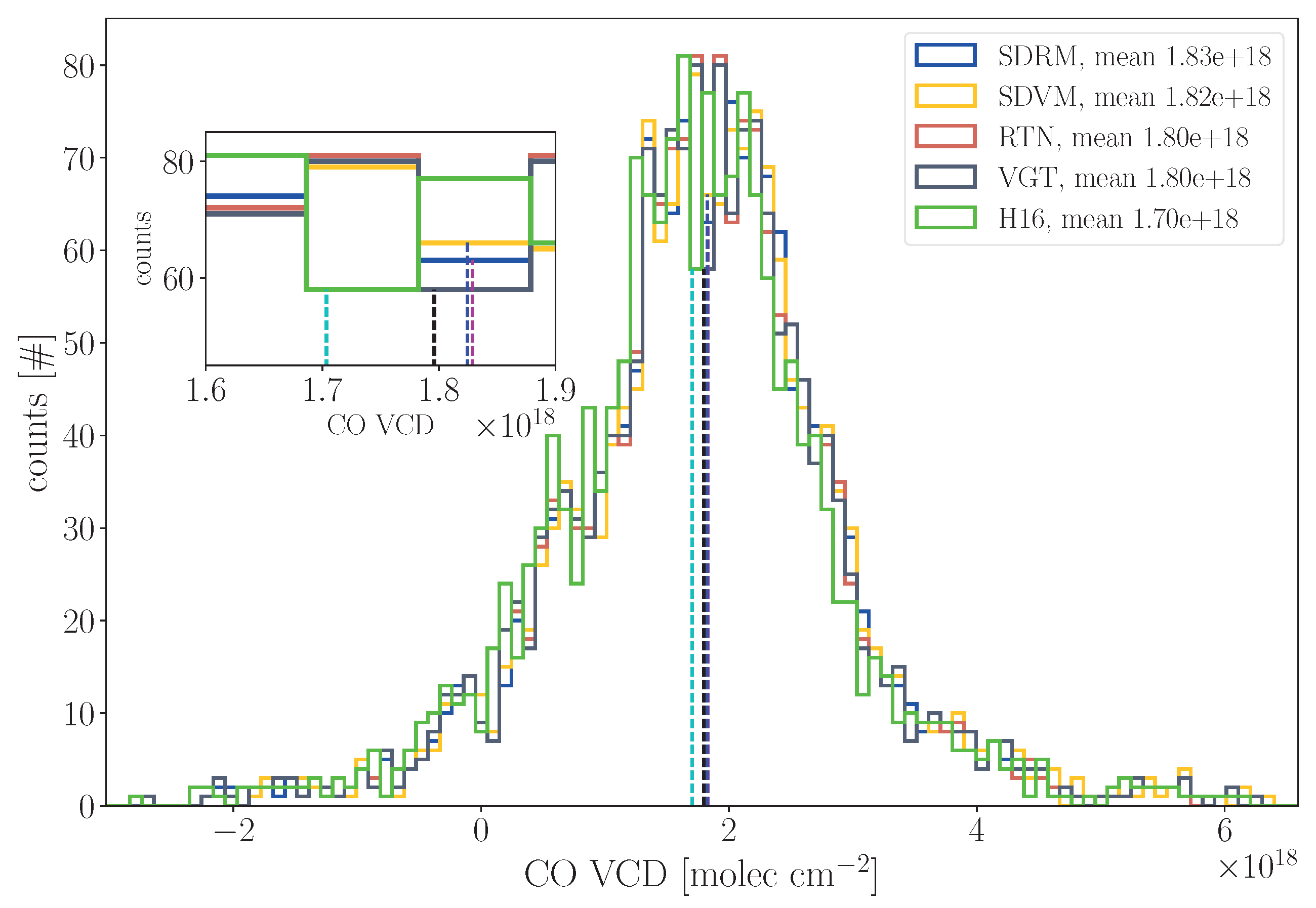
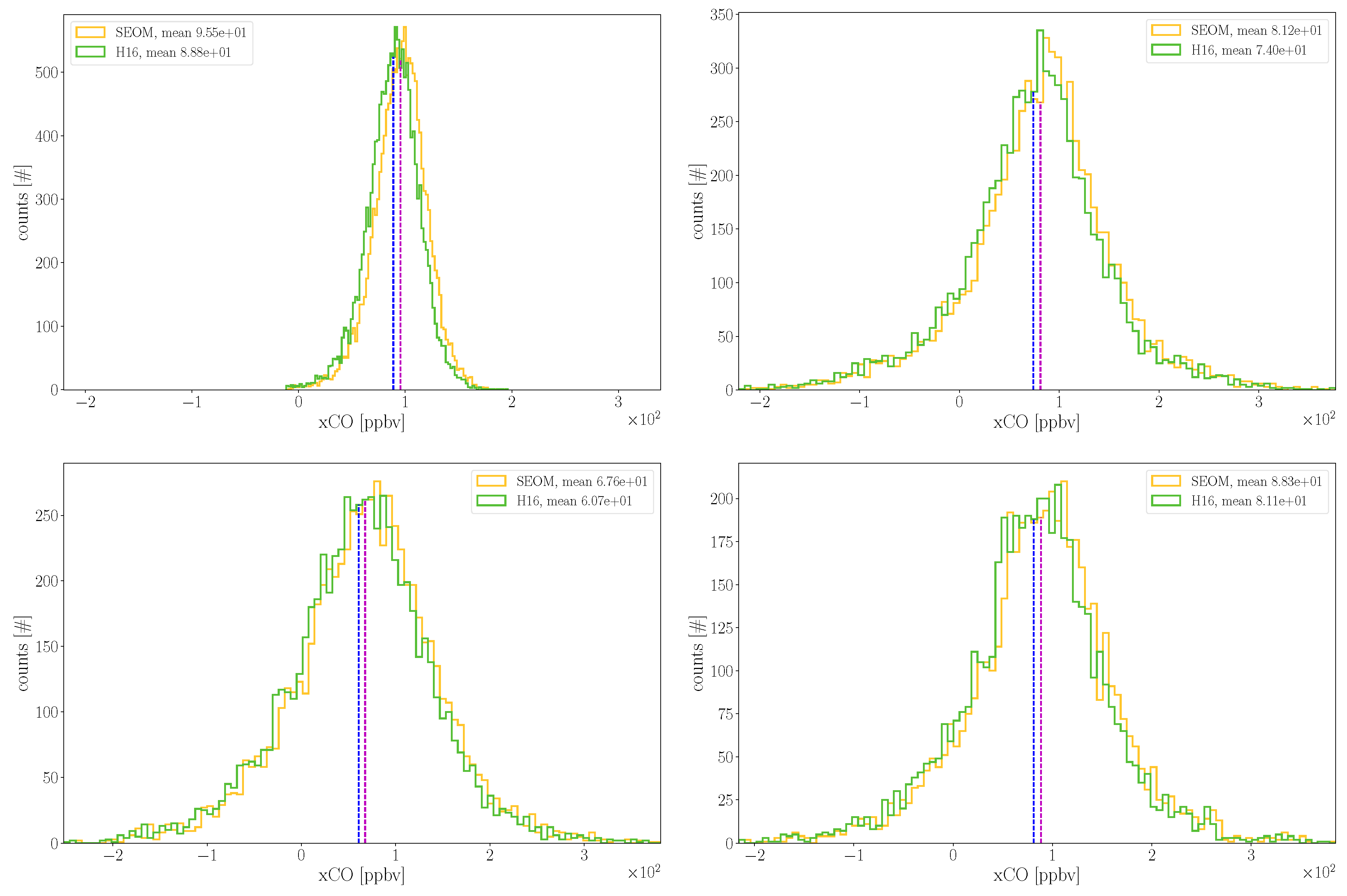
The analysis was extended to different climatological regions (see Table 4). Please note that in the assessment of the spectral fitting residuals it was deemed sufficient to include measurements only from April 2004 since every single SCIAMACHY observation contains 71 measurements that can be analyzed. The second quarter was chosen since small solar zenith angles (SZAs) were preferred for the analysis of retrievals in the (mostly) northern hemispheric regions. Four areas with different conditions in temperature and humidity were selected to discriminate the impact of H 2 O from other molecules. For example, updates of the H 2 O spectroscopy are expected to be more pronounced for measurements over humid areas and less in dry environments. Climatological records show that the attributes dry and hot are well fulfilled in the subtropical Sahara region and a dry and cold climate is prevailing in Siberia. Amazonia is dominated by wet and hot conditions while wet and cold weather is typical for the Canadian West Coast. Since the selected area of the latter region includes adjacent parts of the Pacific Ocean and parts of Alaska it was denoted as CaPaAl. Most ocean pixels are rejected during postprocessing due to high errors in the estimated column scaling factors.
The residual vector in the forward model of the retrieval comprises 71 elements. Table 4 gives the number of observations and relative change in the residual norm regarding HITRAN 2016 for the respective region. The results in Figure 5 show smaller disagreements between the forward model and observations for the retrievals using SEOM data in three of the four examined regions (Amazonia in the second panel shows no significant difference). This finding is in good agreement with the outcome of the analysis for the two orbits presented in Table 3. Especially observations over Siberia and CaPaAl (but also Sahara) reveal that many elements (pixels) of the spectral residuum vector have smaller disagreements with the measured spectrum after convergence. By comparing the position of those pixels on the spectral axis to the lower three panels depicting the optical depths of CO , H 2 O and CH 4 one can observe that some coincide with strong vibrational-rotational transitions of the molecules.

3.2. Differences in CO Mole Fractions

The histogram of x CO for each of the selected regions is depicted in Figure 6. Sahara (top-left) reveals a narrow distribution of CO , only spanning around 200 ppbv including only a few negative values (physically not meaningful on an individual basis). The high surface albedo, resp. reflectivity of this region enhances the SNR and improves the quality of the observed spectra. The narrow distribution of the retrieved xCO is expected to be primarily caused by well represented absorption features of CO , CH 4 (and H 2 O ) in the spectrum, allowing the retrieval to converge within reasonable values for most measurements. However, mean values in xCO differ by 8 ppbv across spectroscopic inputs and therefore spectroscopy clearly has an impact on the retrieval results. In contrast to Sahara the spread of CO mole fractions over Siberia (top-right) is larger but the mean values are similar. The SDVM based retrievals deliver the largest mean, i.e., a 2–8% increase. Amazonia (lower-left) shows a similar result, although medians are lower. xCO values also increase by about 7% in the CaPaAl region (lower-right) for SDVM.
The spatial distribution of xCO differences for SEOM and H16 is depicted in Figure 7. Recall that for the analysis of mole fractions the time period was extended to June 2004 (i.e., it includes three months of observations, April through June 2004). A rise in xCO ranging from around 4% to 11% is observed globally. Particularly in the Sahara Desert and the Arabic Peninsula the updated spectroscopy causes a uniform increase in CO mole fractions by around 7%.
The increase in the x CO is not homogeneous but larger towards higher and lower latitudes. Although the increase of xCO is similar towards the north and the south from the equator in absolute numbers the relative change is larger by around 3% in the southern hemisphere.

3.3. Comparison to NDACC and TCCON

To assess the quality of the updates on the product level a comparison to ground-based measurements was relevant. In our recent validation study [40] we concluded that the global mean bias of the BIRRA CO retrievals is around -14 parts per billion in volume (ppbv) regarding NDACC, and 8 ppbv when compared to TCCON. The discrepancy of the global bias between the two networks is likely caused by a correction factor (1.0672) in the GGG2014 dataset (GGG stands for the whole software package) that is applied to TCCON in order to compensate for spectroscopic uncertainties and ties their calibration to the currently accepted World Meteorological Organization (WMO) gas standard scale (D. G. Feist, personal communication and [74,75,76,77]). NDACC in contrast does not use such a scaling factor.
On one hand, data coverage for NDACC is guaranteed for many sites in 2004 and comparisons of SWIR satellite Level 2 data with MIR (mid infrared) ground-based products have been presented by several groups (e.g., [35,36,78,79,80]). However, it records the fundamental band of CO in the MIR while on the other hand, TCCON retrieves total columns from two broad spectral bands in the first overtone spectrum of CO (details see [76]) which overlaps with our fitting window. In order to compare retrievals with SEOM and HITRAN for at least two TCCON sites, namely Darwin (Australia) and Lauder (New Zealand), it was decided to analyze SCIAMACHY observations from August through October 2005, too. This period constitutes a tradeoff between available observations from reference sites and SCIAMACHY’s SWIR channel performance, although it was already worse compared to previous years ([40] Figure 3).
According to Rodgers and Connor [81] averaging kernels characterize the altitude sensitivity of a retrieval by relating the true and estimated state vectors. With respect to NDACC and TCCON retrievals Zhou et al. ([77] Figure 3) showed that the column averaging kernels are different due to their different retrieval windows, spectral resolution and retrieval schemes. It was found that the TCCON retrieved CO total column underestimates a deviation from the a priori in the lower troposphere, and overestimates it at high altitudes and that NDACC CO retrievals have a good sensitivity to the whole troposphere and lower stratosphere.
The total column averaging kernels for the BIRRA CO retrieval are shown in Figure 8. In accordance with findings by Gloudemans et al. [28], Buchwitz et al. [31] the averaging kernels are depending on the SZA and, only to a small extent, on the observation angle, a priori trace gas profile and surface albedo. Moreover, as NDACC and TCCON use the HITRAN 2008 (HITRAN 2009 updates for H 2 O and HDO ) and HITRAN 2012 line list, respectively, the dependence on the spectroscopic input (SEOM and HITRAN 2016) was examined and found to be insignificant. However, for a thorough validation with ground-based networks the use of consistent spectroscopic data across platforms would be beneficial.
Based upon these findings, it was concluded that the smoothing error is negligible when comparing strictly clear-sky SCIAMACHY CO total columns to NDACC and TCCON [81] and that a direct comparison is appropriate to estimate the accuracy of the product. This is in good agreement with Borsdorff et al. [35] who also found that for cloud filtered SCIAMACHY total columns the application of the total column averaging kernels is of little importance.
Figure 9 shows the comparison of averaged CO mole fractions retrieved by BIRRA to NDACC and TCCON ground-based reference sites (Appendix Table A1 and Table A2). Systematic differences were calculated according to ([40] Section 2.4 and 3.2.1). A total bias b ¯ of 5.8 ppbv and 12.8 ppbv was found for the SEOM and HITRAN 2016-based retrievals, respectively.
The decreased quality of SCIAMACHY observations over time resulted in an increased number of rejected measurements during postprocessing for the August–October 2005 period thereby decreasing the ensemble of averaged columns. In addition, strict cloud filtering and large scatter of individual measurements are the main reasons for the large standard error of the biases and hence the bias is only significant for two sites when using SEOM compared to six stations when using HITRAN 2016.

4. Summary and Conclusions

In this study, CO total columns were retrieved in the SWIR from a subset of SCIAMACHY measurements in 2003, 2004 and 2005 using SEOM, HITRAN 2016 (and GEISA 2015) line data with corresponding line profiles. The impact of molecular spectroscopy on spectral fitting residuals and the retrieved quantity was examined and quantified.
This analysis lead to the conclusion that the spectroscopy of CO , CH 4 and H 2 O in the 2.3 μ m regime has significant impact on the retrieval of CO in the SWIR. The results show that the spectral residuals are reduced with the new line data and corresponding model. It was found that the impact on the fitted residuals is non-homogeneously distributed across the globe and residuals can be reduced up to 15 %. The updates in the CH 4 and H 2 O lines have a great impact because both molecules are strong absorbers and experienced the most significant updates in SEOM.
The CO mole fractions increased by about ≈ 4–11% reducing the bias to both NDACC and TCCON. It was shown that the largest fraction of the increase is due to updates in the SEOM line parameters and that the line profile only plays a minor role, yet SEOM line data is used optimally when an appropriate line model is chosen. The outcome also confirms recommendations from earlier investigations e.g., by Galli et al. [9] or Checa-García et al. [11], i.e., trace gas retrievals in the SWIR will benefit from improved molecular spectroscopy.
Overall, the findings suggest that the updated line data and models are beneficial for the retrieval of CO from SCIAMACHY in the 2.3 μ m regime. The remaining significant bias at three sites might be reduced when averaging over longer time periods and smaller sampling areas.
Although SEOM has been compiled to meet the accuracy requirements of new operational missions such as TROPOMI/S5p, the results of this study suggest that the updated spectroscopy improves the SWIR Level 2 product of SCIAMACHY, too. These findings are important regarding reprocessing and long-term consistency of the CO product since the compilation of a homogeneous multi-mission time series requires consistent forward modeling and harmonized auxiliary data [82].

Author Contributions

P.H. developed the methods, tools, and strategy for this study and performed all retrievals. F.S. originally designed the forward model and retrieval algorithm. The original draft of the manuscript was prepared by P.H. and then reviewed and edited by both authors. All authors have read and agreed to the published version of the manuscript.

Funding

The first author receives funding from the “DLR-DAAD Research Fellowships” Program which is offered by the German Aerospace Center (DLR) and the German Academic Exchange Service (DAAD).

Acknowledgments

We would like to thank Manfred Birk and Georg Wagner from ESA’s SEOM-IAS Project Team for their effort in producing the new set of spectroscopic line data as well as for the personal communications. The SEOM-IAS data is available from the Open Access platform zenodo.org [19]. Furthermore, we thank Frank Hase and Dietrich Feist for the fruitful discussions and their expertise provided on many aspects regarding ground-based observations. We would also like to thank Thomas Trautmann, Günter Lichtenberg and Mourad Hamidouche for constructive criticism of the manuscript. Finally, we acknowledge the NDACC-InfraredWorking Group and TCCON ground-based Fourier transform spectrometer network for providing data. The NDACC data used in this publication were obtained from sites listed in Appendix Table A1 and are publicly available via ndacc.org. TCCON data were obtained from the TCCON Data Archive, hosted by CaltechDATA, California Institute of Technology, CA (US), doi:10.14291/tccon.archive/1348407. The dataset references are listed in Appendix Table A2.

Conflicts of Interest

The authors declare no conflict of interest.

Abbreviations

The following abbreviations are frequently used in this manuscript:
BIRRABeer Infrared Retrieval Algorithm
GARLICGeneric Atmospheric Radiation Line-by-line Infrared Code
G15GEISA 2015 spectroscopic database
H16HITRAN 2016 spectroscopic database
IRinfrared
lblline-by-line
MIRmid infrared
Py4CAtSPYthon scripts for Computational ATmospheric Spectroscopy
RTNRautian line profile
SCIAMACHYScanning Imaging Absorption SpectroMeter for Atmospheric CHartographY
SEOMSEOM – Improved Atmospheric Spectroscopy (IAS) database
SDVspeed-dependent Voigt line profile
SDVMspeed-dependent Voigt line profile with line-mixing
SDRMspeed-dependent Rautian line profile with line-mixing
SWIRshortwave infrared
VGTVoigt line profile
xCOcarbon monoxide (CO) column-averaged dry-air mole fraction

Appendix A. Impact on Retrieved and Co-Retrieved Quantities

Subsequently, more details on the global variation of the CO mole fractions and individual molecular scaling factors for the different spectroscopic inputs are provided.

Appendix A.1. Differences in the Column Scaling Factors

In general, SEOM-based retrievals show similar differences in the inferred CO regarding both Voigt spectroscopies (see Figure A1 and Figure A2). The smallest disagreements are found in the subtropical regions, especially the Sahara, the Arabic peninsula and some parts of India.
Another pattern unfolds for CH 4 (middle row) as the results indicate some latitudinal dependence in column differences. SDVM retrievals deliver smaller CH 4 scaling factors in the subtropics compared to Rautian retrievals in Appendix Figure A1.
The comparisons of the retrieved H 2 O scaling factors (bottom row) show minor differences for the majority of observations, however, especially around the subpolar regions higher differences are observed.
Finally, the left column in Appendix Figure A3 underlines the fact that the line model has less impact on the scaling factors. The two Voigt spectroscopies in the right column also show the latitudinal pattern in the CH 4 difference.
Figure A1. Spatial distribution of differences in the retrieved profile scaling factors on a 1 × 1 grid from April–June 2004. Left column: SDVM - H16. Right column: RTN - H16 relative difference.
Remotesensing 12 01084 g0a1
Figure A2. Left column: Relative difference of SDVM to G15. Right column: Rautian to G15 relative difference.
Remotesensing 12 01084 g0a2
Figure A3. Left column: Global maps of SDVM to Rautian relative difference for CO , CH 4 and H 2 O scaling factors. Right column: The relative difference of the two Voigt spectroscopies.
Remotesensing 12 01084 g0a3

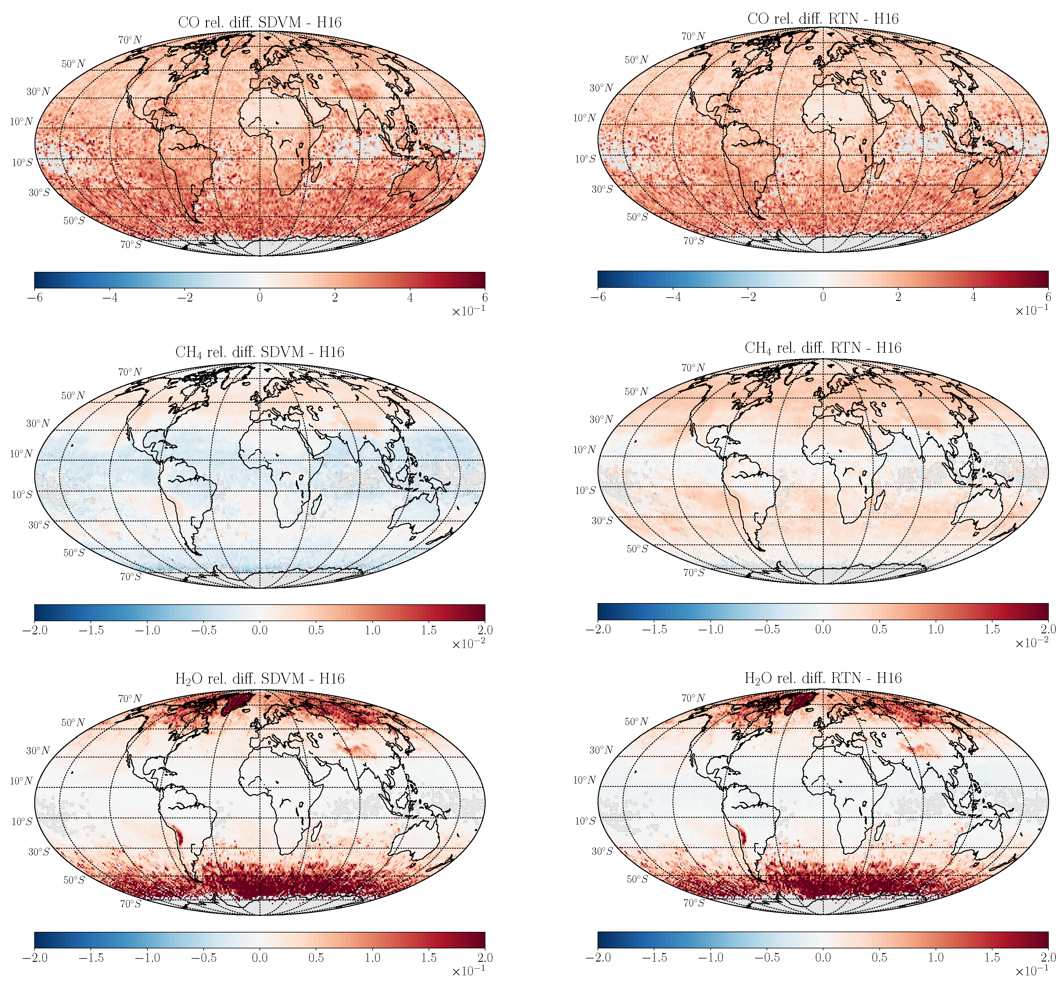
Appendix A.2. Global Map of CO Mole Fractions and Errors

The retrieved CO mole fractions for SDVM are depicted in Appendix Figure A4 (top panel) and reveal largest values in Eastern Asia, and parts of India and Central Africa. The corresponding errors (bottom panel) are smallest in dry regions with low cloud coverage and high surface reflectivity (the Sahara Desert, the Arabian Peninsula, parts of Australia, ...).
Figure A4. (Top) Global distribution of CO column-averaged dry-air mole fractions for the second quarter in 2004. (Bottom) The corresponding errors.
Remotesensing 12 01084 g0a4

Appendix A.3. Line Parameters in SEOM and HITRAN 2016

To accommodate the additional line parameters for the molecules CO , CH 4 and H 2 O in the SEOM database an extended HITRAN format was used (details see ([19] Section 4)). Beside the classical Voigt parameters entries exist for γ 2 , δ 2 , Y and ν vc (Section 2.1.1). In case of CO these higher-order estimates are only available for the strongest lines so the (Voigt) parameters of weaker lines were taken from HITRAN 2016 (see Table 1 and Figure 1).
Although it is possible to retrieve speed-dependent parameters for the first overtone band of CO from HITRAN 2016, there are no entries for CH 4 and H 2 O . More specifically 24 of the 110 CO lines in the 4252.27 4327.90 cm 1 spectral range include the additional speed-dependent Voigt data. However, since CO has a low optical depth and is responsible for only around one percent of absorption in this spectral region the classical Voigt variant of the HITRAN 2016 database was chosen for this study. Also note that the additional parameters are not included in the standard HITRAN format (since HITRAN 2004 with 160 characters [83]) but one needs to create a user-defined output format (at https://hitran.org) specifying the individual parameters. A comparison of the cross-sections k CO for two variants of the HITRAN 2016 line list and SEOM is shown in Appendix Figure A5.
Figure A5. Absorption cross-sections of CO at reference pressure and temperature for SEOM and two variants of the HITRAN 2016 line data (upper panel). In the lower panel the classical HITRAN case (Voigt) is subtracted from the SDR and SDV cross-sections using SEOM and HITRAN, respectively. The SDR-Voigt difference (blue) is moderate in the line center and wings and small in the transition region. In contrast, the SDV-Voigt difference (red) is large only in the line center and drops sharply in the line wings.
Remotesensing 12 01084 g0a5

Appendix B. NDACC Data Providers

The NDACC data in this publication were obtained from sites listed in Appendix Table A1. The data are publicly available via http://www.ndacc.org.
Table A1. NDACC sites used in this publication along with the stations’ representative and cooperating institution.
NDACC SiteCoorperating Institutions
BremenProf Dr Justus Notholt
Institute of Environmental Physics; University of Bremen, Germany
ZugspitzeDr Ralf Sussmann
Institute for Meteorology and Climate Research; Karlsruhe Institute of Technology, Germany
IzanaDr Emilio Cuevas Agulló
Izana Atmospheric Research Center; AEMET – Meteorological State Agency, Spain
JungfraujochDr Emmanuel Mahieua
University of Liége, Belgium
KirunaDr Uwe Raffalski
Institute of Space Physics, Sweden
ThuleDr Niels Larsen
Danish Climate Center; Danish Meteorological Institute, Denmark
TorontoDr Kimberly Strong
Department of Physics; University of Toronto, Canada

Appendix C. TCCON Data Providers

The TCCON data were obtained from sites listed in Appendix Table A2. The TCCON Data Archive is hosted by CaltechDATA, California Institute of Technology, CA (US), doi: https://doi.org/10.14291/tccon.archive/1348407. The Darwin TCCON site is supported by ARC grants DP160101598, DP140101552, DP110103118 and DP0879468, and NASA grants NAG5-12247 and NNG05-GD07G.
Table A2. Total Carbon Column Observing Network (TCCON) sites with the references to the data used in this publication.
TCCON SiteReference
DarwinGriffith et al. [84]
LauderSherlock et al. [85]

References

  1. Perrin, A. Review on the existing spectroscopic databases for atmospheric applications. In Spectroscopy from Space; NATO Science Series II; Demaison, J., Sarka, K., Cohen, E., Eds.; Springer Netherlands: Dordrecht, The Netherlands, 2001; Volume 20, pp. 235–258. [Google Scholar]
  2. Flaud, J.; Oelhaf, H. Infrared spectroscopy and the terrestrial atmosphere. C. R. Phys. 2004, 5, 259–271. [Google Scholar] [CrossRef]
  3. Payan, S.; de La Noë, J.; Hauchecorne, A.; Camy-Peyret, C. A review of remote sensing techniques and related spectroscopy problems. C. R. Phys. 2005, 6, 825–835. [Google Scholar] [CrossRef]
  4. Chance, K. Ultraviolet and visible spectroscopy and spaceborne remote sensing of the Earth’s atmosphere. Comp. R. Phys. 2006, 6, 836–847. [Google Scholar] [CrossRef]
  5. Flaud, J.; Perrin, A.; Picquet-Varrault, B.; Gratien, A.; Orphal, J.; Doussin, J. Quantitative Spectroscopy and Atmospheric Measurements. In Remote Sensing of the Atmosphere for Environmental Security; NATO Security through Science Series; Perrin, A., Ben Sari-Zizi, N., Demaison, J., Eds.; Springer: Dordrecht, The Netherlands, 2006; Volume 14, pp. 107–121. [Google Scholar] [CrossRef]
  6. Flaud, J.; Picquet-Varrault, B.; Gratien, A.; Orphal, J.; Doussin, J. Synergistic Use of Different Atmospheric Instruments: What about the Spectral Parameters? In Proceedings of the First Atmospheric Science Conference; Lacoste, H., Ed.; ESA: Frascati, Italy, 2006; Volume SP-628. [Google Scholar]
  7. Feng, X.; Zhao, F.S. Effect of changes of the HITRAN database on transmittance calculations in the near-infrared region. J. Quant. Spectrosc. Radiat. Transf. 2009, 110, 247–255. [Google Scholar] [CrossRef]
  8. Kratz, D.P. The sensitivity of radiative transfer calculations to the changes in the HITRAN database from 1982 to 2004. J. Quant. Spectrosc. Radiat. Transf. 2008, 109, 1060–1080. [Google Scholar] [CrossRef]
  9. Galli, A.; Butz, A.; Scheepmaker, R.A.; Hasekamp, O.; Landgraf, J.; Tol, P.; Wunch, D.; Deutscher, N.M.; Toon, G.C.; Wennberg, P.O.; et al. CH4, CO, and H2O spectroscopy for the Sentinel-5 Precursor mission: An assessment with the Total Carbon Column Observing Network measurements. Atmos. Meas. Tech. 2012, 5, 1387–1398. [Google Scholar] [CrossRef] [Green Version]
  10. Scheepmaker, R.A.; Frankenberg, C.; Galli, A.; Butz, A.; Schrijver, H.; Deutscher, N.M.; Wunch, D.; Warneke, T.; Fally, S.; Aben, I. Improved water vapour spectroscopy in the 4174–4300 cm−1 region and its impact on SCIAMACHY HDO/H2O measurements. Atmos. Meas. Tech. 2013, 6, 879–894. [Google Scholar] [CrossRef] [Green Version]
  11. Checa-García, R.; Landgraf, J.; Galli, A.; Hase, F.; Velazco, V.; Tran, H.; Boudon, V.; Alkemade, F.; Butz, A. Mapping spectroscopic uncertainties into prospective methane retrieval errors from Sentinel-5 and its precursor. Atmos. Meas. Tech. 2015, 8, 3617–3629. [Google Scholar] [CrossRef] [Green Version]
  12. Gordon, I.; Rothman, L.; Hill, C.; Kochanov, R.; Tan, Y.; Bernath, P.; Birk, M.; Boudon, V.; Campargue, A.; Chance, K.; et al. The HITRAN2016 molecular spectroscopic database. J. Quant. Spectrosc. Radiat. Transf. 2017, 203, 3–69. [Google Scholar] [CrossRef]
  13. Jacquinet-Husson, N.; Armante, R.; Scott, N.; Chédin, A.; Crépeau, L.; Boutammine, C.; Bouhdaoui, A.; Crevoisier, C.; Capelle, V.; Boonne, C.; et al. The 2015 edition of the GEISA spectroscopic database. J. Mol. Spectrosc. 2016, 327, 31–72, New Visions of Spectroscopic Databases, Volume II. [Google Scholar] [CrossRef] [Green Version]
  14. Pickett, H.; Poynter, R.; Cohen, E.; Delitsky, M.; Pearson, J.; Müller, H. Submillimeter, millimeter, and microwave spectral line catalog. J. Quant. Spectrosc. Radiat. Transf. 1998, 60, 883–890. [Google Scholar] [CrossRef]
  15. Endres, C.P.; Schlemmer, S.; Schilke, P.; Stutzki, J.; Müller, H.S. The Cologne Database for Molecular Spectroscopy, CDMS, in the Virtual Atomic and Molecular Data Centre, VAMDC. J. Mol. Spectrosc. 2016, 327, 95–104, New Visions of Spectroscopic Databases, Volume II. [Google Scholar] [CrossRef] [Green Version]
  16. Nikitin, A.; Lyulin, O.; Mikhailenko, S.; Perevalov, V.; Filippov, N.; Grigoriev, I.; Morino, I.; Yokota, T.; Kumazawa, R.; Watanabe, T. GOSAT-2009 methane spectral line list in the 5550–6236 cm−1 range. J. Quant. Spectrosc. Radiat. Transf. 2010, 111, 2211–2224. [Google Scholar] [CrossRef]
  17. Campargue, A.; Leshchishina, O.; Wang, L.; Mondelain, D.; Kassi, S.; Nikitin, A. Refinements of the WKMC empirical line lists (5852–7919 cm−1) for methane between 80 K and 296 K. J. Quant. Spectrosc. Radiat. Transf. 2012, 113, 1855–1873. [Google Scholar] [CrossRef]
  18. Nikitin, A.; Lyulin, O.; Mikhailenko, S.; Perevalov, V.; Filippov, N.; Grigoriev, I.; Morino, I.; Yoshida, Y.; Matsunaga, T. GOSAT-2014 methane spectral line list. J. Quant. Spectrosc. Radiat. Transf. 2015, 154, 63–71. [Google Scholar] [CrossRef]
  19. Birk, M.; Wagner, G.; Loos, J.; Mondelain, D.; Campargue, A. ESA SEOM–IAS—Spectroscopic Parameters Database 2.3 μm Region [Data set]. Zenodo. 2017. Available online: https://zenodo.org/record/1009126#.XnyN7q19iXl (accessed on 8 March 2019).
  20. Buchwitz, M.; Burrows, J. Retrieval of CH4, CO, and CO2 total column amounts from SCIAMACHY near-infrared nadir spectra: Retrieval algorithm and first results. In Proceedings of the 10th International Symposium Remote Sensing—Remote Sensing of Clouds and the Atmosphere VIII, Barcelona, Spain, 8–12 September 2003. [Google Scholar]
  21. Pan, L.; Gille, J.; Edwards, D.; Bailey, P.; Rodgers, C. Retrieval of tropospheric carbon monoxide for the MOPITT experiment. J. Geophys. Res. 1998, 103, 32277–32290. [Google Scholar] [CrossRef]
  22. Kuze, A.; Suto, H.; Nakajima, M.; Hamazaki, T. Thermal and near infrared sensor for carbon observation Fourier-transform spectrometer on the Greenhouse Gases Observing Satellite for greenhouse gases monitoring. Appl. Opt. 2009, 48, 6716–6733. [Google Scholar] [CrossRef]
  23. Crisp, D.; Atlas, R.; Breon, F.M.; Brown, L.; Burrows, J.; Ciais, P.; Connor, B.; Doney, S.; Fung, I.; Jacob, D.; et al. The Orbiting Carbon Observatory (OCO) mission. Adv. Space Res. 2004, 34, 700–709. [Google Scholar] [CrossRef] [Green Version]
  24. Yang, D.; Liu, Y.; Cai, Z.; Chen, X.; Yao, L.; Lu, D. First Global Carbon Dioxide Maps Produced from TanSat Measurements. Adv. Atmos. Sci. 2018, 35, 621–623. [Google Scholar] [CrossRef]
  25. Landgraf, J.; aan de Brugh, J.; Scheepmaker, R.; Borsdorff, T.; Hu, H.; Houweling, S.; Butz, A.; Aben, I.; Hasekamp, O. Carbon monoxide total column retrievals from TROPOMI shortwave infrared measurements. Atmos. Meas. Tech. 2016, 9, 4955–4975. [Google Scholar] [CrossRef] [Green Version]
  26. Frankenberg, C.; Warneke, T.; Butz, A.; Aben, I.; Hase, F.; Spietz, P.; Brown, L.R. Pressure broadening in the 2ν3 band of methane and its implication on atmospheric retrievals. Atm. Chem. Phys. 2008, 8, 5061–5075. [Google Scholar] [CrossRef] [Green Version]
  27. Frankenberg, C.; Bergamaschi, P.; Butz, A.; Houweling, S.; Meirink, J.F.; Notholt, J.; Petersen, A.K.; Schrijver, H.; Warneke, T.; Aben, I. Tropical methane emissions: A revised view from SCIAMACHY onboard ENVISAT. Geophys. Res. Letters 2008, 35, L15811. [Google Scholar] [CrossRef] [Green Version]
  28. Gloudemans, A.; Schrijver, H.; Hasekamp, O.; Aben, I. Error analysis for CO and CH4 total column retrievals from SCIAMACHY 2.3 μm spectra. Atm. Chem. Phys. 2008, 8, 3999–4017. [Google Scholar] [CrossRef] [Green Version]
  29. Oyafuso, F.; Payne, V.; Drouin, B.; Devi, V.; Benner, D.; Sung, K.; Yu, S.; Gordon, I.; Kochanov, R.; Tan, Y.; et al. High accuracy absorption coefficients for the Orbiting Carbon Observatory-2 (OCO-2) mission: Validation of updated carbon dioxide cross-sections using atmospheric spectra. J. Quant. Spectrosc. Radiat. Transf. 2017, 203, 213–223, HITRAN2016 Special Issue. [Google Scholar] [CrossRef]
  30. Borsdorff, T.; aan de Brugh, J.; Schneider, A.; Lorente, A.; Birk, M.; Wagner, G.; Kivi, R.; Hase, F.; Feist, D.G.; Sussmann, R.; et al. Improving the TROPOMI CO data product: Update of the spectroscopic database and destriping of single orbits. Atmos. Meas. Tech. 2019, 12, 5443–5455. [Google Scholar] [CrossRef] [Green Version]
  31. Buchwitz, M.; de Beek, R.; Bramstedt, K.; Noël, S.; Bovensmann, H.; Burrows, J.P. Global carbon monoxide as retrieved from SCIAMACHY by WFM-DOAS. Atm. Chem. Phys. 2004, 4, 1945–1960. [Google Scholar] [CrossRef] [Green Version]
  32. Buchwitz, M.; de Beek, R.; Noël, S.; Burrows, J.P.; Bovensmann, H.; Bremer, H.; Bergamaschi, P.; Körner, S.; Heimann, M. Carbon monoxide, methane and carbon dioxide columns retrieved from SCIAMACHY by WFM-DOAS: Year 2003 initial data set. Atm. Chem. Phys. 2005, 5, 3313–3329. [Google Scholar] [CrossRef] [Green Version]
  33. Frankenberg, C.; Platt, U.; Wagner, T. Retrieval of CO from SCIAMACHY onboard ENVISAT: Detection of strongly polluted areas and seasonal patterns in global CO abundances. Atm. Chem. Phys. 2005, 5, 1639–1644. [Google Scholar] [CrossRef] [Green Version]
  34. Gloudemans, A.; Schrijver, H.; Kleipool, Q.; van den Broek, M.; Straume, A.; Lichtenberg, G.; van Hees, R.; Aben, I.; Meirink, J. The impact of SCIAMACHY near-infrared instrument calibration on CH4 and CO total columns. Atm. Chem. Phys. 2005, 5, 2369–2383. [Google Scholar] [CrossRef] [Green Version]
  35. Borsdorff, T.; Tol, P.; Williams, J.E.; de Laat, J.; aan de Brugh, J.; Nédélec, P.; Aben, I.; Landgraf, J. Carbon monoxide total columns from SCIAMACHY 2.3 μm atmospheric reflectance measurements: Towards a full-mission data product (2003–2012). Atmos. Meas. Tech. 2016, 9, 227–248. [Google Scholar] [CrossRef] [Green Version]
  36. Borsdorff, T.; aan de Brugh, J.; Hu, H.; Nédélec, P.; Aben, I.; Landgraf, J. Carbon monoxide column retrieval for clear-sky and cloudy atmospheres: A full-mission data set from SCIAMACHY 2.3 μm reflectance measurements. Atmos. Meas. Tech. 2017, 10, 1769–1782. [Google Scholar] [CrossRef] [Green Version]
  37. Gimeno García, S.; Schreier, F.; Lichtenberg, G.; Slijkhuis, S. Near infrared nadir retrieval of vertical column densities: Methodology and application to SCIAMACHY. Atmos. Meas. Tech. 2011, 4, 2633–2657. [Google Scholar] [CrossRef] [Green Version]
  38. de Laat, A.; Gloudemans, A.; Schrijver, H.; van den Broek, M.; Meirink, J.; Aben, I.; Krol, M. Quantitative analysis of SCIAMACHY carbon monoxide total column measurements. Geophys. Res. Lett. 2006, 33, L07807. [Google Scholar] [CrossRef] [Green Version]
  39. Lichtenberg, G.; Gimeno García, S.; Schreier, F.; Slijkhuis, S.; Snel, R.; Bovensmann, H. Impact of Level 1 Quality on SCIAMACHY Level 2 Retrieval. In Proceedings of the 38th COSPAR Scientific Assembly, Bremen, Germany, 18–25 July 2010. [Google Scholar]
  40. Hochstaffl, P.; Schreier, F.; Lichtenberg, G.; Gimeno García, S. Validation of Carbon Monoxide Total Column Retrievals from SCIAMACHY Observations with NDACC/TCCON Ground-Based Measurements. Remote Sens. 2018, 10, 223. [Google Scholar] [CrossRef] [Green Version]
  41. Goody, R.; Yung, Y. Atmospheric Radiation—Theoretical Basis, 2nd ed.; Oxford University Press: Oxford, UK, 1989. [Google Scholar]
  42. Liou, K.N. An Introduction to Atmospheric Radiation, 2nd ed.; Academic Press: Cambridge, MA, USA, 2002; p. 583. [Google Scholar]
  43. Zdunkowski, W.; Trautmann, T.; Bott, A. Radiation in the Atmosphere—A Course in Theoretical Meteorology; Cambridge University Press: Cambridge, UK, 2007. [Google Scholar]
  44. Armstrong, B. Spectrum Line Profiles: The Voigt Function. J. Quant. Spectrosc. Radiat. Transf. 1967, 7, 61–88. [Google Scholar] [CrossRef]
  45. Humlíček, J. Optimized computation of the Voigt and complex probability function. J. Quant. Spectrosc. Radiat. Transf. 1982, 27, 437–444. [Google Scholar] [CrossRef]
  46. Weideman, J. Computation of the Complex Error Function. SIAM J. Num. Anal. 1994, 31, 1497–1518. [Google Scholar] [CrossRef]
  47. Schreier, F. Optimized Implementations of Rational Approximations for the Voigt and Complex Error Function. J. Quant. Spectrosc. Radiat. Transf. 2011, 112, 1010–1025. [Google Scholar] [CrossRef]
  48. Tennyson, J.; Bernath, P.; Campargue, A.; Császár, A.; Daumont, L.; Gamache, R.; Hodges, J.; Lisak, D.; Naumenko, O.; Rothman, L.; et al. Recommended isolated-line profile for representing high-resolution spectroscopic transitions (IUPAC Technical Report). Pure Appl. Chem. 2014, 86, 1931–1943. [Google Scholar] [CrossRef] [Green Version]
  49. Berman, P. Speed-dependent collisional width and shift parameters in spectral profiles. J. Quant. Spectrosc. Radiat. Transf. 1972, 12, 1321–1342. [Google Scholar] [CrossRef]
  50. Boone, C.; Walker, K.; Bernath, P. Speed–dependent Voigt profile for water vapor in infrared remote sensing applications. J. Quant. Spectrosc. Radiat. Transf. 2007, 105, 525–532. [Google Scholar] [CrossRef]
  51. Boone, C.; Walker, K.; Bernath, P. An efficient analytical approach for calculating line mixing in atmospheric remote sensing applications. J. Quant. Spectrosc. Radiat. Transf. 2011, 112, 980–989. [Google Scholar] [CrossRef]
  52. Kochanov, V.P. Speed-dependent spectral line profile including line narrowing and mixing. J. Quant. Spectrosc. Radiat. Transf. 2016, 177, 261–268. [Google Scholar] [CrossRef]
  53. Varghese, P.; Hanson, R. Collisional narrowing effects on spectral line shapes measured at high resolution. Appl. Opt. 1984, 23, 2376–2385. [Google Scholar] [CrossRef]
  54. Rosenkranz, P. Shape of the 5 mm oxygen band in the atmosphere. IEEE Trans. Antennas Propag. 1975, 23, 498–506. [Google Scholar] [CrossRef]
  55. Strow, L.L.; Tobin, D.C.; Hannon, S.E. A compilation of first-order line-mixing coefficients for CO2 Q-branches. J. Quant. Spectrosc. Radiat. Transf. 1994, 52, 281–294. [Google Scholar] [CrossRef]
  56. Dicke, R.H. The Effect of Collisions upon the Doppler Width of Spectral Lines. Phys. Rev. 1953, 89, 472–473. [Google Scholar] [CrossRef]
  57. Lévy, A.; Lacome, N.; Chackerian, C., Jr. Collisional Line Mixing. In Spectroscopy of the Earth’s Atmosphere and Interstellar Medium; Rao, K., Weber, A., Eds.; Academic Press: Cambridge, MA, USA, 1992; pp. 261–338. [Google Scholar]
  58. Ngo, N.; Lisak, D.; Tran, H.; Hartmann, J.M. An isolated line-shape model to go beyond the Voigt profile in spectroscopic databases and radiative transfer codes. J. Quant. Spectrosc. Radiat. Transf. 2013, 129, 89–100, Erratum: JQSRT 134, 105 (2014). [Google Scholar] [CrossRef]
  59. Tran, H.; Ngo, N.; Hartmann, J.M. Efficient computation of some speed-dependent isolated line profiles. J. Quant. Spectrosc. Radiat. Transf. 2013, 129, 199–203, Erratum: JQSRT 134, 104 (2014). [Google Scholar] [CrossRef]
  60. Malathy Devi, V.; Benner, D.C.; Smith, M.; Mantz, A.; Sung, K.; Brown, L.; Predoi-Cross, A. Spectral line parameters including temperature dependences of self- and air-broadening in the 2-0 band of CO at 2.3μm. J. Quant. Spectrosc. Radiat. Transf. 2012, 113, 1013–1033. [Google Scholar] [CrossRef]
  61. Rothman, L.; Gordon, I.; Babikov, Y.; Barbe, A.; Benner, D.C.; Bernath, P.; Birk, M.; Bizzocchi, L.; Boudon, V.; Brown, L.; et al. The HITRAN2012 molecular spectroscopic database. J. Quant. Spectrosc. Radiat. Transf. 2013, 130, 4–50. [Google Scholar] [CrossRef]
  62. Li, G.; Gordon, I.E.; Rothman, L.S.; Tan, Y.; Hu, S.M.; Kassi, S.; Campargue, A.; Medvedev, E.S. Rovibrational line lists for nine isotopologues of the CO molecule in the X1Σ+ ground electronic state. Astrophys. J. Supp. S. 2015, 216, 15. [Google Scholar] [CrossRef] [Green Version]
  63. Mlawer, E.; Payne, V.; Moncet, J.L.; Delamere, J.; Alvarado, M.; Tobin, D. Development and recent evaluation of the MT-CKD model of continuum absorption. Philos. Trans. Roy. Soc. Lond. Ser. A 2012, 370, 2520–2556. [Google Scholar] [CrossRef] [PubMed] [Green Version]
  64. Jacquinet-Husson, N.; Crepeau, L.; Armante, R.; Boutammine, C.; Chedin, A.; Scott, N.; Crevoisier, C.; Capelle, V.; Boone, C.; Poulet-Crovisier, N.; et al. The 2009 edition of the GEISA spectroscopic database. J. Quant. Spectrosc. Radiat. Transf. 2011, 112, 2395–2445. [Google Scholar] [CrossRef] [Green Version]
  65. Kistler, R.; Collins, W.; Saha, S.; White, G.; Woollen, J.; Kalnay, E.; Chelliah, M.; Ebisuzaki, W.; Kanamitsu, M.; Kousky, V.; et al. The NCEP-NCAR 50-Year Reanalysis: Monthly Means CD-ROM and Documentation. Bull. Am. Met. Soc. 2001, 82, 247–267. [Google Scholar] [CrossRef]
  66. Anderson, G.; Clough, S.; Kneizys, F.; Chetwynd, J.; Shettle, E. AFGL Atmospheric Constituent Profiles (0–120 km ); Technical Report TR-86-0110; Air Force Geophysics Laboratory (AFGL): Hanscom AFB, MA, USA, 1986. [Google Scholar]
  67. Schreier, F.; Gimeno García, S.; Hedelt, P.; Hess, M.; Mendrok, J.; Vasquez, M.; Xu, J. GARLIC—A General Purpose Atmospheric Radiative Transfer Line-by-Line Infrared-Microwave Code: Implementation and Evaluation. J. Quant. Spectrosc. Radiat. Transf. 2014, 137, 29–50. [Google Scholar] [CrossRef] [Green Version]
  68. Hamidouche, M.; Lichtenberg, G. In-Flight Retrieval of SCIAMACHY Instrument Spectral Response Function. Remote Sens. 2018, 10, 401. [Google Scholar] [CrossRef] [Green Version]
  69. Loyola, D. A new cloud recognition algorithm for optical sensors. In Proceedings of the IGARSS ’98. Sensing and Managing the Environment. 1998 IEEE International Geoscience and Remote Sensing. Symposium Proceedings, Seattle, WA, USA, 6–10 July 1998; pp. 572–574. [Google Scholar] [CrossRef]
  70. Kokhanovsky, A.A.; von Hoyningen-Huene, W.; Rozanov, V.V.; Noël, S.; Gerilowski, K.; Bovensmann, H.; Bramstedt, K.; Buchwitz, M.; Burrows, J.P. The semianalytical cloud retrieval algorithm for SCIAMACHY II. The application to MERIS and SCIAMACHY data. Atm. Chem. Phys. 2006, 6, 4129–4136. [Google Scholar] [CrossRef] [Green Version]
  71. Hodges, J.L. The significance probability of the Smirnov two-sample test. Ark. Mat. 1958, 3, 469–486. [Google Scholar] [CrossRef]
  72. Frankenberg, C.; Meirink, J.F.; Bergamaschi, P.; Goede, A.P.H.; Heimann, M.; Körner, S.; Platt, U.; van Weele, M.; Wagner, T. Satellite chartography of atmospheric methane from SCIAMACHY on board ENVISAT: Analysis of the years 2003 and 2004. J. Geophys. Res. 2006, 111, D07303. [Google Scholar] [CrossRef]
  73. Hochstaffl, P.; Gimeno García, S.; Schreier, F.; Hamidouche, M.; Lichtenberg, G. Validation of Carbon Monoxide Vertical Column Densities Retrieved from SCIAMACHY Infrared Nadir Observations. In Proceedings of the Living Planet Symposium, Prague, Czech Republic, 9–13 May 2016. [Google Scholar]
  74. Wunch, D.; Toon, G.C.; Sherlock, V.; Deutscher, N.M.; Liu, C.; Feist, D.G.; Wennberg, P.O. Documentation for the 2014 TCCON Data Release (Version GGG2014.R0). CaltechDATA 2015. [Google Scholar] [CrossRef]
  75. Sussmann, R.; Ostler, A.; Forster, F.; Rettinger, M.; Deutscher, N.M.; Griffith, D.W.T.; Hannigan, J.W.; Jones, N.; Patra, P.K. First intercalibration of column-averaged methane from the Total Carbon Column Observing Network and the Network for the Detection of Atmospheric Composition Change. Atmos. Meas. Tech. 2013, 6, 397–418. [Google Scholar] [CrossRef]
  76. Kiel, M.; Hase, F.; Blumenstock, T.; Kirner, O. Comparison of XCO abundances from the Total Carbon Column Observing Network and the Network for the Detection of Atmospheric Composition Change measured in Karlsruhe. Atmos. Meas. Tech. 2016, 9, 2223–2239. [Google Scholar] [CrossRef] [Green Version]
  77. Zhou, M.; Langerock, B.; Vigouroux, C.; Sha, M.K.; Hermans, C.; Metzger, J.M.; Chen, H.; Ramonet, M.; Kivi, R.; Heikkinen, P.; et al. TCCON and NDACC XCO measurements: Difference, discussion and application. Atmos. Meas. Tech. 2019, 12, 5979–5995. [Google Scholar] [CrossRef] [Green Version]
  78. Sussmann, R.; Buchwitz, M. Initial validation of ENVISAT/SCIAMACHY columnar CO by FTIR profile retrievals at the Ground-Truthing Station Zugspitze. Atm. Chem. Phys. 2005, 5, 1497–1503. [Google Scholar] [CrossRef] [Green Version]
  79. Sussmann, R.; Stremme, W.; Buchwitz, M.; de Beek, R. Validation of ENVISAT/SCIAMACHY columnar methane by solar FTIR spectrometry at the Ground-Truthing Station Zugspitze. Atm. Chem. Phys. 2005, 5, 2419–2429. [Google Scholar] [CrossRef] [Green Version]
  80. Buchholz, R.; Deeter, M.; Worden, H.; Gille, J.; Edwards, D.; Hannigan, J.; Jones, N.; Paton-Walsh, C.; Griffith, D.; Smale, D.; et al. Validation of MOPITT carbon monoxide using ground-based Fourier transform infrared spectrometer data from NDACC. Atmos. Meas. Tech. 2017, 10, 1927–1956. [Google Scholar] [CrossRef] [Green Version]
  81. Rodgers, C.; Connor, B. Intercomparison of remote sounding instruments. J. Geophys. Res. 2003, 108, 4116. [Google Scholar] [CrossRef] [Green Version]
  82. Coldewey-Egbers, M.; Loyola, D.G.; Koukouli, M.; Balis, D.; Lambert, J.C.; Verhoelst, T.; Granville, J.; van Roozendael, M.; Lerot, C.; Spurr, R.; et al. The GOME-type Total Ozone Essential Climate Variable (GTO-ECV) data record from the ESA Climate Change Initiative. Atmos. Meas. Tech. 2015, 8, 3923–3940. [Google Scholar] [CrossRef] [Green Version]
  83. Rothman, L.; Jacquemart, D.; Barbe, A.; Benner, D.C.; Birk, M.; Brown, L.; Carleer, M.; Chackerian, C., Jr.; Chance, K.; Coudert, L.; et al. The HITRAN 2004 molecular spectroscopic database. J. Quant. Spectrosc. Radiat. Transf. 2005, 96, 139–204. [Google Scholar] [CrossRef] [Green Version]
  84. Griffith, D.W.T.; Deutscher, N.M.; Velazco, V.A.; Wennberg, P.O.; Yavin, Y.; Keppel-Aleks, G.; Washenfelder, R.; Toon, G.C.; Blavier, J.F.; Paton-Walsh, C.; et al. TCCON data from Darwin (AU), Release GGG2014.R0. TCCON Data Archive, hosted by CaltechDATA. 2014. Available online: https://data.caltech.edu/records/269l (accessed on 8 March 2019).
  85. Sherlock, V.; Connor, B.; Robinson, J.; Shiona, H.; Smale, D.; Pollard, D. TCCON data from Lauder (NZ), 120HR, Release GGG2014.R0. TCCON Data Archive, hosted by CaltechDATA. 2014. Available online: https://data.caltech.edu/records/281l (accessed on 8 March 2019).
Figure 1. (Top) Line strengths S of CO (left), CH 4 (center), and H 2 O (right) for the three databases in Table 1. While the strong lines are similar in all databases the values do not agree completely. (Bottom) Cross sections of the three molecules at reference pressure (1013.25 hPa) and temperature (296 K).
Remotesensing 12 01084 g001
Figure 2. Histogram of the spectral residuals in orbit 8663 for SEOM and HITRAN 2016.
Remotesensing 12 01084 g002
Figure 3. Difference in the spectral fitting residuals for various spectroscopic inputs and line models. The x-axis of each figure shows the 71 sensor pixels in the CO fitting window. The y-axis in the pseudocolor plots depicts 2090 observations in orbit 13212 from southern to northern latitudes and the lower panels show the median of the residuals for each pixel.
Remotesensing 12 01084 g003
Figure 4. The CO total columns for different line shapes with SEOM input compared to HITRAN in orbit 8663. It shows that SEOM-based retrievals cause larger columns on average (dashed vertical lines).
Remotesensing 12 01084 g004
Figure 5. The upper four panels depict the average residual norm in April 2004 for each available SCIAMACHY pixel for the regions Sahara, Amazonia, Siberia and CaPaAl, respectively. Gaps indicate bad pixels according to the DBPM. The lower three panels show the optical depths of the molecules CO , H 2 O and CH 4 for SEOM and H16 according to US-Standard along with their differences.
Remotesensing 12 01084 g005
Figure 6. The distribution of xCO in the four analyzed regions Sahara (top-left), Siberia (top-right), Amazonia (lower-left) and CaPaAl for the April–June 2004 period. Please note that the retrieved mole fractions in the Sahara span a significant smaller interval.
Remotesensing 12 01084 g006
Figure 7. Spatial distribution of differences in CO mole fractions between SEOM and HITRAN 2016 for the April–June 2004 time period. Gray pixels indicate areas where no retrievals were left after postprocessing.
Remotesensing 12 01084 g007
Figure 8. Total column averaging kernels for the BIRRA CO retrieval [4277.20–4302.90 cm 1 ] in the nadir viewing geometry. The target molecule CO as well as CH 4 reveal a kernel close to unity up to 200 hPa. Measurements with an SZA > 80 are not considered in the retrieval.
Remotesensing 12 01084 g008
Figure 9. Bias between NDACC/TCCON and SCIAMACHY xCO retrievals within 1000 km (distance weighted) of the ground-based reference sites. Stations Darwin and Lauder belong to TCCON while the others are affiliated to NDACC.
Remotesensing 12 01084 g009
Table 1. A comparison of GEISA 2015, HITRAN 2016, and SEOM line data for the 4252.20 4327.90 cm 1 region. The number of spectral lines along with the corresponding range of intensities S, air broadening HWHM γ air and temperature exponents n are shown. In the last two columns the mean of the non-zero air-broadening speed-dependence parameters γ air ( 2 ) and the Dicke narrowing parameters ν vc are given, the number of non-zero values is indicated in the parentheses. In GEISA HDO is treated as an individual species, in the table here these 660 lines are included in the H 2 O entry. Please note that in HITRAN 2016 the CH 4 line at ν ^ = 4270.377259 cm 1 has an incorrect temperature dependence of n = 7.7 (correct n = 0.7 ) and lines at ν ^ = 4255.703126 cm 1 , 4291.829949 cm 1 , and 4291.840848 cm 1 list n = 0 , respectively (I.E.,  Gordon, personal communication). Furthermore, the lower-state energy of the ν ^ = 4270.377259 cm 1 line is incorrectly set to E = 293.1266 cm 1 in GEISA 2015, the correct value is E = 1556.481 cm 1 as in HITRAN 2016.
GasData# Lines S cm 1 / molec cm 2 γ air ( 0 ) [ cm 1 ] n γ air ( 2 ) [ cm 1 ] ν vc [ cm 1 ]
COG15160 1.1 · 10 36 3.6 · 10 21 0.040–0.0790.69
H16110 1.0 · 10 31 3.5 · 10 21 0.042–0.0810.67–0.79
seom110 1.0 · 10 31 3.5 · 10 21 0.042–0.0810.67–0.790.00607(10)0.0047(10)
CH 4 G157213 9.5 · 10 28 5.4 · 10 21 0.034–0.0770.46–0.97
H168375 1.0 · 10 29 5.5 · 10 21 0.034–0.0770.67–0.77
seom6205 6.7 · 10 27 5.5 · 10 21 0.019–0.1820.19–1.820.008405(610)0.00911(65)
H 2 OG151101 8.4 · 10 30 2.2 · 10 23 0.004–0.0960.32–0.69
H161197 1.0 · 10 32 2.2 · 10 23 0.004–0.1090.32–0.73
seom1177 1.4 · 10 30 2.2 · 10 23 0.004–0.1410.31–1.020.007197(35)0.01083(12)
Table 2. Outline of the experiments conducted in the respective sections.
QuantitySpatial ExtendTemporal Coverage
Section 3.1.1spec. residuumsingle orbitsoverpasses in 2003 & 2004
Section 3.1.2spec. residuumregional scaleApril 2004
Section 3.2mole fractionregional scaleApril–June 2004
Section 3.3mole fractionwithin 1000 km from siteApril–June 2004 & August–October 2005
Section Appendix A.1mole fractionglobal scaleApril–June 2004
Table 3. Mean of the norm of the spectral fitting residuals along with the median and standard deviation of the residuum vector for various combinations of line data and models in orbit 8663 (left column) and 13212 (right column). Note that for both the speed-dependent Rautian and speed-dependent Voigt profiles, line-mixing was taken into account.
DataModel E ( σ 2 ) Median ρ std. dev. ρ
SEOMSDRM 1.90 · 10 2 1.71 · 10 2 3.19 · 10 5 1.97 · 10 4 2.86 · 10 3 2.72 · 10 3
SEOMSDVM 1.92 · 10 2 1.70 · 10 2 3.49 · 10 5 2.00 · 10 4 2.87 · 10 3 2.72 · 10 3
SEOMRautian 1.92 · 10 2 1.73 · 10 2 4.78 · 10 5 1.94 · 10 4 2.88 · 10 3 2.74 · 10 3
SEOMVoigt 1.93 · 10 2 1.73 · 10 2 4.32 · 10 5 2.03 · 10 4 2.88 · 10 3 2.73 · 10 3
HITRAN 2016Voigt 1.96 · 10 2 1.75 · 10 2 3.23 · 10 5 1.94 · 10 4 2.91 · 10 3 2.75 · 10 3
GEISA 2015Voigt 1.98 · 10 2 1.77 · 10 2 2.45 · 10 5 2.07 · 10 4 2.92 · 10 3 2.76 · 10 3
Table 4. The examined regions along with their spatial extent, rate of filtered observations and number of measurements after postprocessing in April 2004. The relative change in the norm of the spectral fitting residual is given in the last column.
RegionLatitudeLongitudeDiscarded Obs.# Survivors Δ σ 2 / σ H 16 2
Sahara18 N–30 N004 W–026 E14%1234−6.89%
Siberia55 N–66 N066 E–095 E60%1104−10.25%
Amazonia08 S–03 N078 W–051 W54%10840.14%
CaPaAl49.5 N–58.5 N117 W–140 W49%683−14.71%

