Joint Inversion of GPS, Leveling, and InSAR Data for The 2013 Lushan (China) Earthquake and Its Seismic Hazard Implications


Abstract

1. Introduction
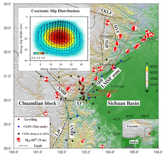
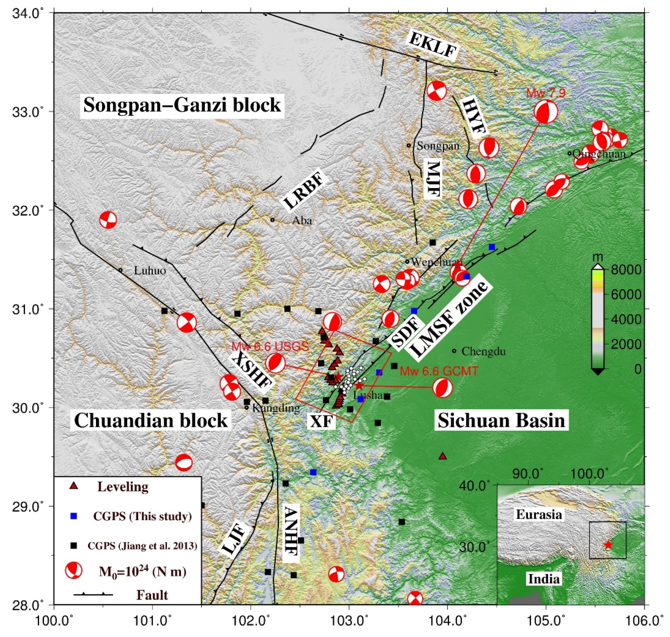
2. Tectonic Background
3. Data and Methods
3.1. GPS Data
3.2. Leveling Data
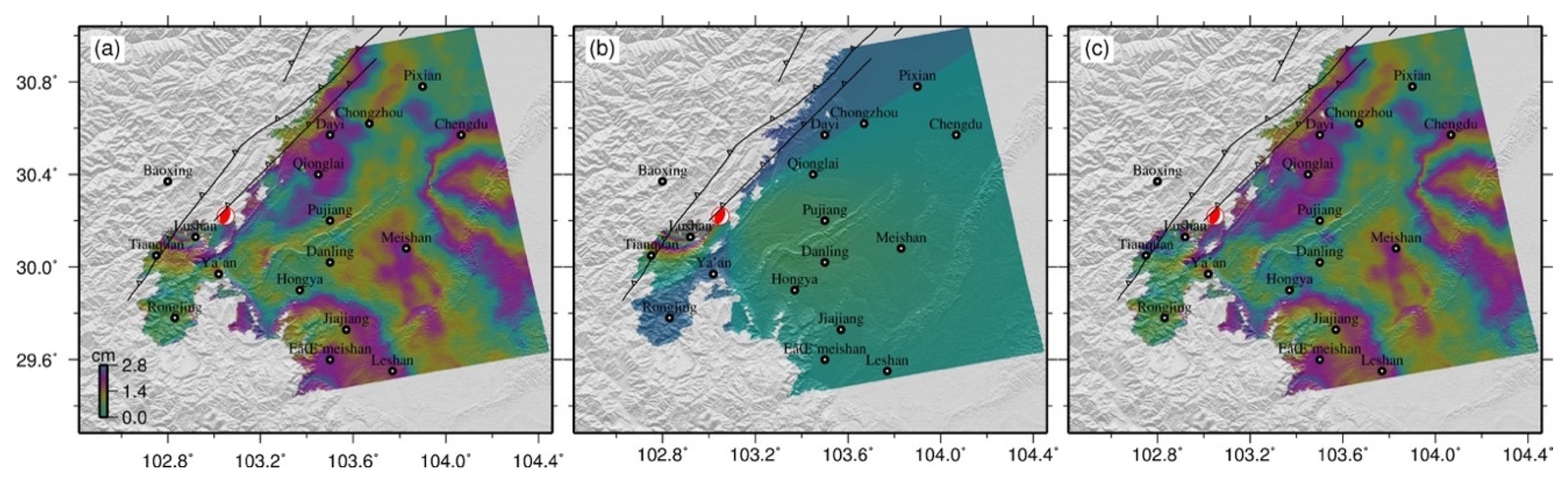
3.3. InSAR Data
4. Joint Inversion
4.1. Uniform Slip Inversion
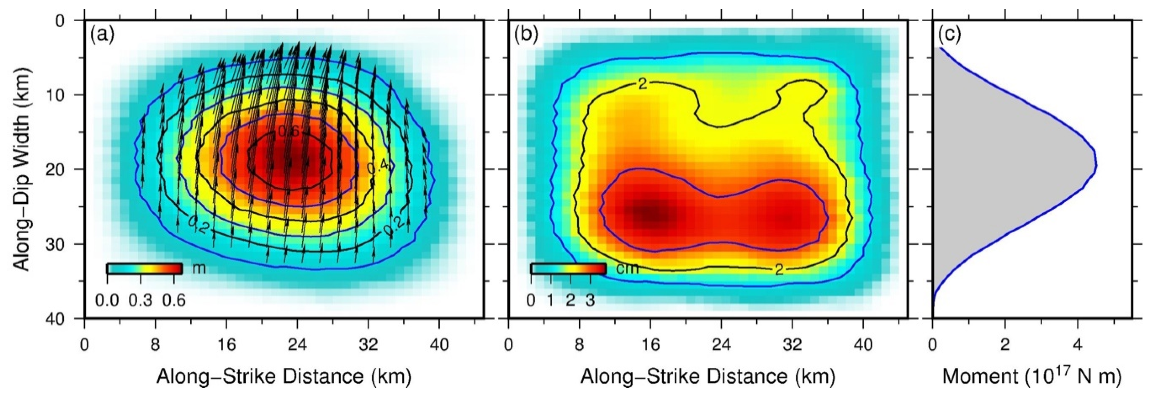
4.2. Distributed Slip Inversion
4.3. Checkerboard Tests
5. Coseismic Stress Changes
6. Discussion
7. Conclusions
Author Contributions
Funding
Acknowledgments
Conflicts of Interest
References
- Chen, X.; Cui, P.; You, Y.; Yang, Z.; Kong, Y. Secondary mountain disasters induced by the 4·20 Lushan earthquake and disaster mitigation. Earth Sci. Front. 2013, 20, 29–30. (In Chinese) [Google Scholar]
- Liu, J.; Yi, G.; Zhang, Z.W.; Guan, Z.J.; Ruan, X.; Long, F.; Du, F. Introduction to the Lushan, Sichuan M7.0 earthquake on 20 April 2013. Chin. J. Geophys. 2013, 56, 1404–1407. (In Chinese) [Google Scholar] [CrossRef]
- USGS. Available online: https://earthquake.usgs.gov/earthquakes/eventpage/usb000gcdd/executive (accessed on 10 November 2019).
- Zhang, Y.; Xu, L.S.; Chen, Y.T. Rupture process of the Lushan 4.20 earthquake and preliminary analysis on the disaster-causing mechanism. Chin. J. Geophys. 2013, 56, 1408–1411. (In Chinese) [Google Scholar] [CrossRef]
- Zhao, B.; Gao, Y.; Huang, Z.B.; Zhao, X.; Li, D.H. Double difference relocation, focal mechanism and stress inversion of Lushan Ms 7.0 earthquake sequence. Chin. J. Geophys. 2013, 56, 3385–3395. (In Chinese) [Google Scholar] [CrossRef]
- Liu, R.F.; Chen, Y.T.; Zou, L.Y.; Chen, S.F.; Liang, J.H.; Zhang, L.W.; Han, X.J.; Ren, X.; Sun, L. Determination of parameters for the 20 April 2013 Lushan Mw6.7 (Ms7.0) earthquake in Sichuan Province. Acta Seismol. Sin. 2013, 35, 652–660. (In Chinese) [Google Scholar]
- Liu, C.; Zheng, Y.; Ge, C.; Xiong, X.; Hsu, H. Rupture process of the Ms7.0 Lushan earthquake, 2013. Sci. China Earth Sci. 2013, 56, 1187–1192. [Google Scholar] [CrossRef]
- Xu, X.; Chen, G.; Yu, G.H.; Cheng, J.; Xi-Bin, T.; Zhu, A.; Wen, X.-Z. Seismogenic structure of Lushan earthquake and its relationship with Wenchuan earthquake. Earth Sci. Front. 2013, 20, 11–20. (In Chinese) [Google Scholar]
- Wang, W.; Hao, J.L.; Yao, Z.X. Preliminary result for rupture process of Apr. 20, 2013, Lushan Earthquake, Sichuan, China. Chin. J. Geophys. 2013, 56, 1412–1417. (In Chinese) [Google Scholar] [CrossRef]
- Xu, X.; Wen, X.; Han, Z.; Chen, G.; Li, C.; Zheng, W.; Zhang, S.; Ren, Z.; Xu, C.; Tan, X.; et al. Lushan MS7.0 earthquake: A blind reserve-fault event. Chin Sci Bull. 2013, 58, 3437–3443. [Google Scholar] [CrossRef]
- Jiang, Z.; Wang, M.; Wang, Y.; Wu, Y.; Che, S.; Shen, Z.; Bürgmann, R.; Sun, J.; Yang, Y.; Liao, H.; et al. GPS constrained coseismic source and slip distribution of the 2013 Mw6.6 Lushan, China, earthquake and its tectonic implications. Geophys. Res. Lett. 2014, 41, 407–413. [Google Scholar] [CrossRef]
- Hao, M.; Wang, Q.; Liu, L.; Shi, Q. Interseismic and coseismic displacements of the Lushan Ms7.0 earthquake inferred from leveling measure-ments. Chin. Sci. Bull. 2014, 59, 5129–5135. [Google Scholar] [CrossRef]
- Liu, Y.; Wang, C.; Shan, X.; Zhang, G.; Qu, C. Result of SAR differential interferometry for the co-seismic deformation and source parameter of the Ms7.0 Lushan earthquake. Chin. J. Geophys. 2014, 57, 2495–2506. [Google Scholar] [CrossRef]
- Deng, M.; Sun, H.; Xu, J.; Zhu, Y. Theoretical simulation of co-seismic and post-seismic deformations and gravity changes of Lushan earthquake. Earth Sci. J. China Univ. Geosci. 2014, 39, 1373–1382. (In Chinese) [Google Scholar] [CrossRef]
- Yang, G.H.; Zhu, S.; Liang, H.; Yang, B. Pre-seismic and co-seismic deformation of Ms 7.0 earthquake in Lushan. Geomat. Inf. Sci. Wuhan Univ. 2015, 40, 121–127. (In Chinese) [Google Scholar]
- Tan, K.; Wang, Q.; Ding, K.; Li, H.; Zou, R.; Nie, Z.S.; Wang, D.; Yang, S.; Qiao, X. Rupture models of the 2013 Lushan earthquake constrained by near field displacements and its tectonic implications. Chin. J. Geophys. Chin. Ed. 2015, 58, 3169–3182. (In Chinese) [Google Scholar] [CrossRef]
- Liu, Q.; Wen, X.Z.; Shao, Z.G. Joint inversion for coseismic slip of the 2013 MS7.0 Lushan earthquake from GPS, leveling and strong motion observations. Chin. J. Geophys. 2016, 59, 2113–2125. (In Chinese) [Google Scholar] [CrossRef]
- Zhang, G.; Hetland, E.; Shan, X.; Martin, V.; Liu, Y.; Zhang, Y.; Qu, C. Triggered slip on a back reverse fault in the Mw6.8 2013 Lushan, China earthquake revealed by joint inversion of local strong motion accelerograms and geodetic measurements. Tectonophysics 2016, 672–673, 24–33. [Google Scholar] [CrossRef]
- Xu, C.J.; Zhou, L.X.; Yin, Z. Construction and geodesy slip inversion analysis of 2013 Ms 7.0 Lushan in China earthquake’s curved fault model. Geomat. Inf. Sci. Wuhan Univ. 2017, 42, 1665–1672. (In Chinese) [Google Scholar]
- Huang, Y.; Qiao, X.; Freymueller, J.T.; Wang, Q.; Yang, S.; Tan, K.; Zhao, B. Fault geometry and slip distribution of the 2013 Mw 6.6 Lushan earthquake in China constrained by GPS, InSAR, leveling, and strong motion data. J. Geophys. Res. Solid Earth 2019, 124, 7341–7353. [Google Scholar] [CrossRef]
- Shan, B.; Xiong, X.; Zheng, Y.; Diao, F. Stress changes on major faults caused by 2013 Lushan earthquake, and its relationship with 2008 Wenchuan earthquake. Sci. China Earth Sci. 2013. (In Chinese) [Google Scholar] [CrossRef]
- Wang, M.; Jia, D.; Shaw, H.J.; Hubbard, J.; Plesch, A.; Li, Y.; Liu, B. The 2013 Lushan earthquake: Implications for seismic hazards posed by the range front blind thrust in the Sichuan basin, China. Geology 2014, 42, 915–918. [Google Scholar] [CrossRef]
- Wang, Z.; Su, J.; Liu, C.; Cai, X. New insights into the generation of the 2013 Lushan Earthquake (Ms 7.0), China. J. Geophys. Res. Solid Earth 2015, 120, 3507–3526. [Google Scholar] [CrossRef]
- Lin, X.; Chu, R.; Zeng, X. Rupture processes and Coulomb stress changes of the 2017 Mw 6.5 Jiuzhaigou and 2013 Mw 6.6 Lushan earthquakes. Earth Planets Space 2019, 71, 81. [Google Scholar] [CrossRef]
- Wang, Y.; Wang, E.; Shen, Z.; Wang, M.; Gan, W.; Qiao, X.; Meng, G.; Li, T.; Tao, W.; Yang, Y.; et al. GPS-constrained inversion of present-day slip rates along major faults of the Sichuan–Yunnan region. China Sci. China Earth Sci. 2008, 51, 1267–1283. [Google Scholar] [CrossRef]
- Densmore, A.L.; Ellis, M.A.; Li, Y.; Zhou, R.; Hancock, G.S.; Richardson, N. Active tectonics of the Beichuan and Pengguan faults at the eastern margin of the Tibetan Plateau. Tectonics 2007, 26, TC4005. [Google Scholar] [CrossRef]
- Shen, Z.; Lu, J.; Wang, M.; Burgmann, R. Contemporary crustal deformation around southeast borderland of Tibetan plateau. J. Geophys. Res. 2005, 110, B11409. [Google Scholar] [CrossRef]
- Li, Y.; Jia, D.; Wang, M.; Shaw, J.; He, J.; Lin, A.; Xiong, L.; Rao, G. Structural geometry of the source region for the 2013 Mw 6.6 Lushan earthquake: Implication for earth- quake hazard assessment along the Longmen Shan. Earth Planet. Sci. Lett. 2014, 390, 275–286. [Google Scholar] [CrossRef]
- Fang, L.; Wu, J.; Wang, W.; Du, W.; Su, J.; Wang, C.; Cai, Y. Aftershock observation and analysis of the 2013 Ms 7.0 Lushan earthquake. Seismol. Res. Lett. 2015, 86, 1135–1142. [Google Scholar] [CrossRef]
- Ziewonski, A.M.; Chou, T.A.; Woodhouse, J.H. Determination of earthquake source parameters from waveform data for studies of global and regional seismicity. J. Geophys. Res. 1981, 86, 2825–2852. [Google Scholar] [CrossRef]
- Ekström, G.; Nettles, M.; Dziewonski, A.M. The global CMT project 2004-2010: Centroid-moment tensors for 13,017 earthquakes. Phys. Earth Planet. Inter. 2012, 200–201, 1–9. [Google Scholar] [CrossRef]
- Dach, R.; Lutz, S.; Walser, P.; Fridez, P. (Eds.) Bernese GNSS Software Version 5.2. In User Manual, Astronomical Institute, University of Bern; Bern Open Publishing: Bern, Switzerland, 2015. [Google Scholar] [CrossRef]
- Kouba, J.; Héroux, P. Precise point positioning using IGS orbit and clock products. GPS Solut. 2001, 5, 12–28. [Google Scholar] [CrossRef]
- Yao, Y.B. Research on the Alorithm and Realization of Post-Processing for GPS Precise Positioning and Orbit Determination; Wuhan University: Wuhan, China, 2004. [Google Scholar]
- Gao, C.; Zhao, Y.; Wan, D. The weight determination of the double difference observation in GPS carrier phase positioning. Sci. Surv. Mapp. 2005, 30, 28–32. [Google Scholar]
- Borkowski, K.M. Accurate algorithms to transform geocentric to geodetic coordinates. Bull. Géod. 1989, 63, 50–56. [Google Scholar] [CrossRef]
- Wang, J.X. Correlations among parameters in seven-parameter transformation model. J. Geod. Geodyn. 2007, 27, 43–46. [Google Scholar]
- Li, J.L.; Liu, L.; Qiao, S.B.; Guo, L. Discussion on the determination of transformation parameters of 3D cartesian coordinates. Sci. Surv. Mapp. 2010, 35, 76–78. [Google Scholar]
- Werner, C.; Wegmller, U.; Strozzi, T.; Wiesmann, A. GAMMA SAR and Interferometric Processing Software. In Proceedings of the ERS-Envisat Symposium, Gothenburg, Sweden, 16–20 October 2001. [Google Scholar]
- Rosen, P.A.; Hensley, S.; Peltzer, G.; Simons, M. Updated repeat orbit interferometry package released. EOS Trans. Am. Geophys. Union 2004, 85, 47. [Google Scholar] [CrossRef]
- Goldstein, R.; Werner, C. Radar interferogram filtering for geophysical applications. Geophys. Res. Lett. 1998, 25, 4035–4038. [Google Scholar] [CrossRef]
- Goldstein, R.; Zebker, H.; Werner, C. Satellite radar interferometry: Two-dimensional phase unwrapping. Radio Sci. 1988, 23, 713–720. [Google Scholar] [CrossRef]
- Hanssen, R.F. Radar Interferometry: Data Interpretation and Error Analysis; Kluwer Academic Publishers: Dordrecht, The Netherlands, 2001. [Google Scholar]
- Okada, Y. Surface deformation due to shear and tensile faults in a half-space. Bull. Seismol. Soc. Am. 1985, 75, 1135–1154. [Google Scholar]
- Lohman, R.B.; Simons, M. Some thoughts on the use of InSAR data to constrain models of surface deformation: Noise structure and data downsampling. Geochem. Geophys. Geosyst. 2005, 6, 359–361. [Google Scholar] [CrossRef]
- Xu, C.; Liu, Y.; Wen, Y.; Wang, R. Coseismic slip distribution of the 2008 Mw 7.9 Wenchuan earthquake from joint inversion of GPS and InSAR data. Bull. Seismol. Soc. Am. 2010, 100, 2736–2749. [Google Scholar] [CrossRef]
- Feng, W.; Li, Z.; Elliott, J.R.; Fukushima, Y.; Hoey, T.; Singleton, A.; Cook, R.; Xu, Z. The 2011 MW 6.8 Burma earthquake: Fault constraints provided by multiple SAR techniques. Geophys. J. Int. 2013, 195, 650–660. [Google Scholar] [CrossRef]
- Parsons, B.; Wright, T.; Rowe, P.; Andrews, J.; Jackson, J.; Walker, R.; Khatib, M.; Talebian, M.; Bergman, E.; Engdahl, E. The 1994 Sefidabeh (eastern Iran) earthquakes revisited: New evidence from satellite radar interferometry and carbonate dating about the growth of an active fold above a blind thrust fault. Geophys. J. Int. 2006, 164, 202–217. [Google Scholar] [CrossRef]
- King, G.C.P.; Stein, R.S.; Lin, J. Static stress changes and the triggering of earthquakes. Bull. Seismol. Soc. Am. 1994, 78, 935–953. [Google Scholar]
- Ziv, A.; Rubin, A.M. Static stress transfer and earthquake triggering: No lower threshold in sight? J. Geophys. Res. Solid Earth 2000, 105, 13631–13642. [Google Scholar] [CrossRef]
- Toda, S.; Stein, R.S.; Richards-Dinger, K.; Bozkurt, S.B. Forecasting the evolution of seismicity in southern California: Animations built on earthquake stress transfer. J. Geophys. Res. Solid Earth 2005, 110, 361–368. [Google Scholar] [CrossRef]
- Steck, L.K.; Phillips, W.S.; Mackey, K.; Begnaud, M.L.; Stead, R.J.; Rowe, C.A. Seismic tomography of crustal P and S across Eurasia. Geophys. J. Int. 2009, 177, 81–92. [Google Scholar] [CrossRef]
- Shan, B.; Xiong, X.; Zheng, Y.; Diao, F. Stress changes on major faults caused by Mw7.9 Wenchuan earthquake, May 12, 2008. Sci. China Earth Sci. 2013, 52, 593–601. [Google Scholar] [CrossRef]
- Wang, R.; Lorenzo-Martín, F.; Roth, F. PSGRN/PSCMP—A new code for calculating co-and post-seismic deformation, geoid and gravity changes based on the viscoelastic-gravitational dislocation theory. Comput. Geosci. 2006, 32, 527–541. [Google Scholar] [CrossRef]
- Wen, Y.; Xu, C.; Liu, Y.; Jiang, G. Deformation and source parameters of the 2015 Mw 6.5 earthquake in Pishan, Western China, from Sentinel-1A and ALOS-2 data. Remote Sens. 2016, 8, 134. [Google Scholar] [CrossRef]
- Jiang, G.; Wen, Y.; Liu, Y.; Xu, X.; Fang, L.; Chen, G.; Gong, M.; Xu, C. Joint analysis of the 2014 Kangding, southwest China, earthquake sequence with seismicity relocation and InSAR inversion. Geophys. Res. Lett. 2015, 42, 3273–3281. [Google Scholar] [CrossRef]
- Mai, P.M.; Spudich, P.; Boatwright, J. Hypocenter locations in finite-source rupture models. Bull. Seismol. Soc. Am. 2005, 95, 965–980. [Google Scholar] [CrossRef]
- Ma, K.; Chan, C.; Stein, R. Response of seismicity to Coulomb stress triggers and shadows of the 1999 Mw = 7.6 Chi-Chi, Taiwan, earthquake. J. Geophys Res. 2005. [Google Scholar] [CrossRef]
- Wessel, P.; Smith, W.H.F.; Scharroo, R.; Luis, J.; Wobbe, F. Generic mapping tools: Improved version released. Eos Trans. Am. Geophys. Union 2013, 94, 409–410. [Google Scholar] [CrossRef]


| Site | Long. (°E) | Lat. (°N) | E (mm) | Se (mm) | N (mm) | Sn (mm) | U (mm) | Su (mm) |
|---|---|---|---|---|---|---|---|---|
| BECH | 104.45 | 31.62 | 0.5 | 1.3 | −1.3 | 1.5 | −3.1 | 5.8 |
| DUJY | 103.66 | 30.98 | 0.3 | 0.9 | 0 | 1.7 | 0.8 | 4.4 |
| HANY | 102.63 | 29.34 | 0.1 | 1.6 | 0.6 | 1.7 | −2.6 | 3.9 |
| LS01 | 103.38 | 30.11 | −15.8 | 1.4 | 7.1 | 1.6 | −2.0 | 4.9 |
| LS02 | 103.27 | 30.67 | 1.4 | 1.8 | 3.6 | 2.5 | −14.3 | 13.1 |
| LS03 | 102.68 | 30.98 | 3.5 | 1.3 | −2.4 | 1.7 | −2.5 | 4.7 |
| LS04 | 103.29 | 29.84 | −6.1 | 1.1 | 6.3 | 1.7 | −0.7 | 4.1 |
| LS05 | 102.92 | 30.16 | −8.9 | 1.1 | −67.3 | 1.6 | 82.6 | 3.5 |
| LS06 | 102.81 | 30.30 | −3.2 | 1.7 | −5.4 | 1.7 | 19.5 | 3.7 |
| LS07 | 102.71 | 30.44 | 24.7 | 1.1 | −18.2 | 1.5 | −7.3 | 2.8 |
| LS08 | 102.74 | 30.71 | 6.8 | 0.9 | −10.2 | 1.6 | −1.3 | 3.8 |
| LS09 | 101.86 | 30.95 | 4.5 | 2.0 | −2.7 | 1.4 | 2.5 | 5.5 |
| LS10 | 102.15 | 30.06 | 3.7 | 1.8 | −1.6 | 1.3 | −7.6 | 4.3 |
| MINS | 103.11 | 30.08 | −21.0 | 1.9 | 18.7 | 2.2 | −8.3 | 6.1 |
| MZHU | 104.19 | 31.33 | 0.7 | 1.4 | −1.1 | 1.6 | −3.1 | 6.0 |
| QLA1 | 103.30 | 30.35 | −10.6 | 1.4 | 0.2 | 1.5 | −1.5 | 4.6 |
| QLAI | 103.45 | 30.42 | −4.7 | 1.4 | −1.1 | 1.5 | −0.1 | 4.7 |
| SCDF | 101.12 | 30.98 | 1.8 | 1.3 | −1.3 | 1.5 | 1.0 | 4.5 |
| SCJL | 101.50 | 29.01 | −0.8 | 2.1 | −0.5 | 1.4 | −4.5 | 6.3 |
| SCMB | 103.53 | 28.84 | 0.2 | 1.8 | 0 | 1.5 | −0.2 | 3.9 |
| SCMN | 102.17 | 28.33 | 1.2 | 1.4 | −1.3 | 1.3 | 3.8 | 4.7 |
| SCMX | 103.85 | 31.67 | 1.0 | 1.2 | −0.6 | 1.6 | −2.0 | 4.1 |
| SCSM | 102.35 | 29.23 | 0.1 | 1.7 | −0.5 | 1.5 | −2.9 | 3.3 |
| SCTQ | 102.76 | 30.07 | −7.9 | 1.1 | −19.4 | 1.8 | 4.6 | 4.7 |
| SCXD | 102.43 | 28.30 | −0.7 | 1.9 | −2.3 | 2.0 | −1.8 | 8.2 |
| SCXJ | 102.37 | 31.00 | 3.1 | 1.2 | −2.6 | 1.0 | −2.6 | 4.7 |
| SCYX | 102.51 | 28.65 | 0 | 2.7 | −1.8 | 1.6 | 2.9 | 7.0 |
| YAAN | 103.01 | 29.98 | −6.2 | 1.1 | 6.5 | 1.3 | −2.9 | 4.9 |
| YAAN | 103.01 | 29.98 | −6.2 | 1.1 | 6.5 | 1.3 | −2.9 | 4.9 |
| Site | LONG. (°E) | LAT. (°N) | U (mm) | (mm) |
|---|---|---|---|---|
| Y165A | 102.86 | 30.01 | 0 | 0 |
| CKFY001 | 102.88 | 30.03 | −8.2 | 0.9 |
| FXG2167 | 102.89 | 30.03 | 4.3 | 0.6 |
| DD42 | 102.89 | 30.06 | 5.1 | 0.9 |
| DD41 | 102.90 | 30.08 | 16.2 | 0.8 |
| DD40 | 102.91 | 30.10 | 30.0 | 0.7 |
| DF37A(09) | 102.93 | 30.14 | 59.4 | 1.2 |
| DD36 | 102.93 | 30.18 | 130.3 | 1.0 |
| DD35 | 102.94 | 30.21 | 198.4 | 0.8 |
| DD32 | 102.86 | 30.27 | 82.1 | 1.7 |
| DD30 | 102.83 | 30.25 | 55.9 | 1.3 |
| DF29(09) | 102.81 | 30.28 | 25.6 | 0.8 |
| DD28 | 102.79 | 30.30 | 10.6 | 1.0 |
| DD23 | 102.83 | 30.41 | −16.2 | 1.6 |
| DD22 | 102.85 | 30.44 | −8.3 | 0.9 |
| DF23(09) | 102.88 | 30.47 | −10.5 | 1.0 |
| DF21(09) | 102.90 | 30.55 | 3.6 | 1.5 |
| DF20(09) | 102.88 | 30.59 | −3.3 | 1.1 |
| DD15 | 102.79 | 30.64 | −3.7 | 1.5 |
| DF17(09) | 102.75 | 30.67 | −21.0 | 1.1 |
| DF16(09) | 102.75 | 30.71 | −13.1 | 1.1 |
| DD8 | 102.73 | 30.77 | −8.1 | 1.4 |
| Source | Long | Lat | Length | Depth | Width | Strike | Dip | Rake | Slip | Mw |
|---|---|---|---|---|---|---|---|---|---|---|
| (°E) | (°N) | (km) | (km) | (km) | (°) | (°) | (°) | (m) | ||
| Uni. Model a | 102.984 | 30.258 | 24.3 | 7.4 | 15.0 | 208.0 | 45.0 | 81.6 | 0.71 | 6.56 |
| ±0.7 km | ±0.8 km | ±2.3 | ±1.3 | ±3.4 | ±4.7 | ±1.3 | ±7.9 | ±0.17 | ||
| Dist. Model b | 103.052 | 30.228 | 45 | 0 | 40 | 208.0 | 43.0 | 83.0 | 0.33 | 6.58 |
| USGS BW c | 102.888 | 30.308 | - | 19.0 | - | 216 | 47 | 93 | - | 6.5 |
| GCMT d | 103.12 | 30.22 | - | 21.9 | - | 212 | 42 | 100 | - | 6.6 |
| Zhang et al. [18] | - | - | 45 | 0 | 40 | 210 | 63/40/10 | - | 1.6 | 6.8 |
| Huang et al. [20] | - | - | 208.5 | 42.1 | 1.2 | 6.53 | ||||
| Jiang et al. [11] | 102.940 | 30.179 | 22.5 | 7.7 | 17.0 | 208.0 | 43.0 | 81.7 | 0.70 | 6.6 |
© 2020 by the authors. Licensee MDPI, Basel, Switzerland. This article is an open access article distributed under the terms and conditions of the Creative Commons Attribution (CC BY) license (http://creativecommons.org/licenses/by/4.0/).
Share and Cite
Li, Z.; Wen, Y.; Zhang, P.; Liu, Y.; Zhang, Y. Joint Inversion of GPS, Leveling, and InSAR Data for The 2013 Lushan (China) Earthquake and Its Seismic Hazard Implications. Remote Sens. 2020, 12, 715. https://doi.org/10.3390/rs12040715
Li Z, Wen Y, Zhang P, Liu Y, Zhang Y. Joint Inversion of GPS, Leveling, and InSAR Data for The 2013 Lushan (China) Earthquake and Its Seismic Hazard Implications. Remote Sensing. 2020; 12(4):715. https://doi.org/10.3390/rs12040715
Chicago/Turabian StyleLi, Zhicai, Yangmao Wen, Peng Zhang, Yang Liu, and Yong Zhang. 2020. "Joint Inversion of GPS, Leveling, and InSAR Data for The 2013 Lushan (China) Earthquake and Its Seismic Hazard Implications" Remote Sensing 12, no. 4: 715. https://doi.org/10.3390/rs12040715
APA StyleLi, Z., Wen, Y., Zhang, P., Liu, Y., & Zhang, Y. (2020). Joint Inversion of GPS, Leveling, and InSAR Data for The 2013 Lushan (China) Earthquake and Its Seismic Hazard Implications. Remote Sensing, 12(4), 715. https://doi.org/10.3390/rs12040715