Abstract
Coastal woodlands, notable for their floristic diversity and ecosystem service values, are increasingly under threat from a range of interacting biotic and abiotic stressors. Monitoring these complex ecosystems has traditionally been confined to field-scale vegetation surveys; however, remote sensing applications are increasingly becoming more viable. This study reports on the application of field-based monitoring and remote sensing/(Geographic Information System) GIS to interrogate trends in Banksia coastal woodland decline (Kings Park, Perth and Western Australia) and documents the patterns, and potential drivers, of tree mortality over the period 2012–2016. Application of geographic object-based image analysis (GEOBIA) at a park scale was of limited benefit within the closed-canopy ecosystem, with manual digitisation methods feasible only at the smaller transect scale. Analysis of field-based identification of tree mortality, crown-specific spectral characteristics and park-scale change detection imagery identified climate-driven stressors as the likely primary driver of tree mortality in the woodland, with vegetation decline exacerbated by secondary factors, including water stress and low system resilience occasioned by the inability to access the water table and competition between tree species. The results from this paper provide a platform to inform monitoring efforts using airborne remote sensing within coastal woodlands.
1. Introduction
The geographical and ecological position that coastal woodlands occupy means these ecosystems are under threat from a changing climate [1,2] and an expanding coastal-focused urban population [3,4]. Globally, urban populations are expected to grow by 1.35 million by 2030 [5], with local Greater Perth populations increasing by approximately 1% each year from 2016–2019 [6]. Traditionally, land clearance driven by these expanding urban populations has had the greatest impact on coastal woodland systems [7]; however, tree mortality [1,8,9] is posing a significant risk to remnant coastal woodlands. Tree mortality is defined as a reduction in overall plant health over a period of time, which, in the most extreme case, can include tree death [10,11]. This can include decline in overall ecosystem structure and function [12,13], changes in relative competitive capability of specific species relative to one another or the loss of less resilient species, resulting in a transition of the system floristics [7,14,15,16]. The ability to monitor time-space patterns of tree health is therefore an important component in determining potential drivers of tree mortality and informing management of coastal woodlands [4,17,18].
1.1. Drivers of Coastal Woodland Decline
Drivers of coastal woodland decline include biotic and abiotic stressors (summarised in Table 1) [4], including pathogenic infestation, competition between species, changes to the fire regime, shifts in the water table depth, climate change (herein referring to temperature and rainfall anomalies not consistent with long-term baseline trends) and episodic disturbances.

Table 1.
A summary of the biotic and abiotic stressors on woodland vegetation, their causes and techniques for measuring and sensing patterns of tree mortality.
Pathogens, such as Phytophthora cinnamomi Rands (“Phytophthora”) in the southwest of Western Australia (SWWA), are a main biotic threat in vegetated areas that significantly alters the canopy structuring and ground cover of the affected regions, leading to secondary adverse impacts on flora regeneration, nutrient cycling, overall productivity and biodiversity [19]. Similarly, insect infestations may induce crown thinning and eventually the death of a tree [20]. Other biotic factors include competition arising from invasive species [21,22,23] and from coloniser species such as A. fraseriana that typically have a high tree density and are able to out-compete surrounding species for available water, nutrient or light resources. This significantly alters water and soil nutrient regimes, potentially leading to keystone species decline [9].
Coastal woodlands within a fringing urban development are also associated with a transition from a natural to modified fire regime, typically defined by incidental and uncontrolled burns. Natural fire regimes minimise competition between trees by reducing tree density, indirectly alleviating water stress [10,24] and stimulating tree vigour. For example, Banksia species are known to establish prolifically after fire events, with the highest densities of B. menziesii and B. attenuata recorded in regions subject to fire burning [25]; conversely, suppression of fire leads to an observable reduction in tree vigour attributed to increased competition between tree species [9,10]. Accumulation of carbon-rich organic matter or “fuel load” as a result of fire suppression poses an additional risk to the woodland in the event of an unplanned fire [10]. The impact on ecosystem health arising from the natural to modified fire regime transition has been a key motivator of prescribed controlled burns [26].
Accelerated tree mortality in eighty countries, including Australia, has been linked to water stress associated with global climate change (i.e., elevated temperatures and inadequate rainfall) [2,10,27]. Where elevated temperatures are accompanied by a reduction in rainfall, recharge of the vadose zone and underlying groundwater may be impeded [28,29,30], and species accessing stored soil moisture and shallow groundwater may exhibit increased susceptibility to tree mortality. Water vulnerability can also interact with episodic weather events, such as high winds and extreme heat waves [31], that place further stress on vegetation. The ability to access water resources, strategies to tolerate negative water potentials and regulate stomatal control will impact on the ability of specific species to modulate the exacerbated impact of combined stressors [32].
Under conditions of increased development of water resources (increased water abstraction) or changes in climate, which manifests in changes to the frequency, magnitude and duration of heat waves and drought conditions, water stress in trees will become acute and adversely influence their growth and vigour [27,33]. Where these abiotic stressors act together and potentially in association with biotic stressors (refer to Table 1), ecosystem health is likely to decline [4].
1.2. Measuring and Sensing Tree Mortality in Coastal Woodlands
Understanding whether single or multiple biotic and abiotic stressors are driving woodland decline and mortality requires rich space-time data at the scale of individual trees and overall ecosystem health, and that allows determination of between-species responses. Conventional field-based vegetation surveys are focused at plant-to-plot scales (metres to tens of metres or hectares) [4,35,36] and powerful for determining individual and species-specific responses [18]. Determining broader patterns of tree mortality is more challenging, particularly in biodiverse ecosystems. However, remotely sensed imagery can play an important role in assessing vegetation conditions at a park scale (hectares to square kilometres) [27,37,38]. This can be at the scale of individual trees with centimetre to sub-metre data from drones or airborne imagery to broader ecosystem responses with coarser (satellite) data [13].
At the finest scale, observational and physiological field studies conducted on individual leaves, plants or stand/transects scale monitor changes in plant health [39]. Observational field studies capture changes in foliar health or general degradation of the plant [24]. Physiological field studies may include various measurements of tree water status (for example, measuring sap flow and leaf water potential) to ascertain whether the predominant tree stressor is one which places the tree under significant water stress [40,41]. These conventional field-based methods for monitoring vegetation status can provide highly accurate data but are expensive, time-consuming and generally restricted to the plant-to-plot scales [35,38].
Remotely sensed imagery can overcome some of these limitations in providing park-scale multitemporal spatial data from which to assess trends in vegetation condition [13,27]. It also enables analysis of plant health variation over space and time in the context of factors such as water availability (water table depth), plant density and competition and the correspondence of tree death to times of known extreme heat and/or drought conditions [8]. Both thermal data [9,42,43] and multispectral imagery and related vegetation indices have been used to monitor water stress in vegetation [13]. Vegetation indices typically incorporate combinations of the blue, green and red regions of visible light and also near- and mid-infrared regions based on the understanding of the way that vegetation under healthy or stressed conditions absorbs light more strongly in the blue and red regions of the electromagnetic spectrum while reflecting in the near-infrared (NIR) and green [27,44]. Digital multispectral images can include the raw bands data or reflectance values (e.g., red, green, blue and NIR) or may be combined into true colour RGB imagery or false colour imagery [36].
1.3. Study Aim
The aim of the study is to combine field-based monitoring and aerial multispectral imagery to investigate spatiotemporal trends in vegetation conditions of a nationally significant and at-risk Environmental Protection and Biodiversity Conservation (EPBC)-listed coastal woodland ecosystem (Banksia woodland), Kings Park bushland, Perth Western Australia over a five-year period (2012–2016). Within this overall aim, potential drivers of decline within the coastal Banksia woodland will be considered, including: water availability (water table depth), plant density and competition and climate.
2. Materials and Methods
2.1. Study Site and Climatology
The Kings Park bushland (Figure 1) is located approximately 1 km from Central Perth, within the Swan Coastal Plain bioregion (31.96°S, 115.83°E) [45]. The remnant bushland covers an area of approximately 267 ha [9] with the hot dry summers and cool wet winters redolent of a Mediterranean climate [14]. The dominant tree species within the bushland include Banksia, Allocasuarina and Eucalypt species, as well as a number of perennial flowering plants [21]. Banksia woodlands are significant on the bioregional scale, with forty-six of the documented eighty genera of species residing in Australia [46]. These woodlands offer a number of ecological services, including their importance as nectar sources for a range of birdlife and insects [9].
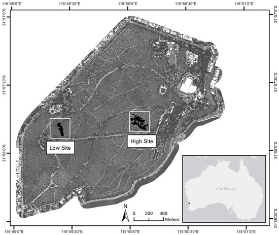
Figure 1.
The two study sites within the Kings Park bushland. Imagery provided by SpecTerra Systems Pty Ltd.
Two research sites (high and low site) previously monitored by Challis et al. [47] were used for this study within the Kings Park bushland (Figure 1). The high and low sites cover a total area of 6360 m2 and 5400 m2, respectively, with the high site situated 50 m above the groundwater table and the low site 9–20 m above the water table, with the likelihood of groundwater access for tree species within the lower site that may buffer water availability.
Inter-annual and intra-annual trends in rainfall (Figure 2A,B, respectively) and temperature (Figure 2C) for the study site indicate frequent below-average rainfall conditions, aside from 2011 and 2013, with frequent above-average maximum temperature events across the study period (2012–2016), many within the hot/dry summer period (Figure 2C, red areas). Anomalies in rainfall (Figure 2B) and temperature (Figure 2C) are calculated as the difference of the mean monthly (rainfall) and weekly running average (temperature) from the long-term monthly average for the corresponding month, calculated across the reference period of meteorological station operation (1993–2018, [48]).
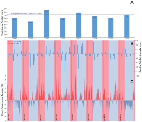
Figure 2.
Total annual rainfall (mm) (A), mean monthly rainfall anomaly (based on 1993–2018 average) (B) and weekly mean temperature anomaly (°C) (C) (difference from 1993–2018 average for corresponding month) across 2009–2016 for Perth, Western Australia at the Perth Metro Station [48], with red areas denoting the hot/dry and blue the cool/wet seasons. Hot-dry seasons: December, January, February, March and April (DJFMA). Cool-wet seasons: May, June, July, August, September, October and November (MJJASON).
2.2. Field Data Acquisition and Processing
Field data was collected at the high and low sites (Figure 1) between October 2015 and February 2016 and appended to the data collected by Challis et al. [47] in the summer of 2013–14. A Trimble R10 Real Time Kinematic Differential Global Positioning System (RTK-DGPS; Yuma, Trimble, USA), which allows high-accuracy measurements (<0.015 m XYZ error) with subpixel (0.5 m) accuracy, was used to map the locations of living and dead trees. Dominant species were identified and tree health evaluated following the methodology of Challis et al. [47]. Measurements of tree canopy extent and trunk diameter were recorded using a standard measuring tape and a diameter at breast height (DBH) tape, respectively, and a TruPulse 200/B Laser Rangefinder for tree height. Ecophysiological measurements of tree mortality, canopy survival and the degree of resprouting was also recorded in accordance with the classification criteria summarised in Table 2. The year of tree mortality (where applicable) was determined for the past three years (Criteria 1, Table 2) by inspection of the remaining bark, general decomposition of tree and leaf presence or absence. Secondly, the proportion of dead branches and general observations of foliar loss provided an indication of the percentage canopy cover (Criteria 2, Table 2), and thirdly, the presence of resprouting trees was classified according to the strength of epicormic resprouts (Criteria 3, Table 2).
Table 2.
Three criteria applied to individual trees in Kings Park to evaluate tree health and mortality status. Adapted from Challis et al. [49].
In-field observation of weed presence and insect/pathogenic infection was also undertaken during field surveys.
While the methodology of Challis et al. [47] was replicated for data collection, not all trees initially mapped in 2013–14 were resurveyed in the summer of 2015–16; however, both transects were traversed, and all trees that had died within the previous two years were mapped. Young seedlings below the height threshold of 1.37 m [50] and seedlings without a reported DBH reading were excluded from mapped output.
2.3. Imagery Acquisition and Preprocessing
High-resolution airborne multispectral (HiRAMS) four-band narrow-bandwidth imagery (Table 3) at 0.5 m resolution was acquired over Kings Park by SpecTerra Systems Pty Ltd. (“SpecTerra”) (Perth, Western Australia) (https://www.specterra.com.au/). SpecTerra operate the HiRAMS sensor and acquisition parameters to specify the same spectral band-passes and near-identical individual image collection location to ensure near-to-same (<5°) view angle for all pixels, clear sky conditions and consistent image preprocessing.
Table 3.
High-resolution airborne multispectral (HiRAMS) bands and corresponding wavelengths (µm) collected by SpecTerra services.
SpecTerra collected and processed imagery acquired for 2012 (23/03/2012), 2014 (23/03/2014), 2015 (23/02/2015 and 23/03/2015) and 2016 (27/02/2016). In-house workflow addresses image orthorectification, bi-directional reflectance distribution function (BRDF) correction, with band miss-registration <0.2 pixels [51,52]. A multivariate alteration detection (MAD) approach adapted from Nielsen et al. [53] is used to identify sufficient invariant targets from which a precise radiometric calibration of raw data to like values based on the approach of Furby and Campbell [54] using a linear regression method on the mosaicked imagery [51,54]. SpecTerra data for their multiyear performance of imagery radiometric calibration precision across multiple image sets and jobs relative to their pseudo-invariant calibration targets is (R2 values): Blue = 0.921, Green = 0.947, Red = 0.956 and NIR = 0.949 (SpecTerra Systems Pty Ltd., unpublished data).
To validate the radiometric precision of the supplied imagery used in this study, we selected 2012 as a baseline and an initial dataset of likely pseudo-invariant pixels (n = 67; irrigated grass (n = 14), roads and paths (n = 25), sun-illuminated hardcourt tennis courts (n = 12), waterbodies (n = 8) and building roofs (n = 8)). Initial screening based on Pearson’s regression (R2) values for all years and bands relative to 2012 showed likely bias by surface type, with sun-illuminated hardcourt tennis courts (R2 = 0.921) and waterbodies (R2 = 0.725) relatively consistent, whereas the other three surface types were unstable and not likely actual pseudo-invariant targets (building roofs R2 = 0.447, irrigated grass R2 = 0.365 and roads and paths R2 = 0.293) and were excluded. Using only pseudo-invariant targets from sun-illuminated hardcourt tennis courts and waterbodies (n = 20), we calculate Pearson’s regression (R2), Nash-Sutcliffe [55] efficiency (NSE; see Equation (1)) and the Wilmott [56] index of agreement (d; see Equation (2)) across imagery time series and for each band:
where Pi is the radiometric pixel value in the pair image, is the radiometric value in 2012 baseline and is the mean of the observations of the 2012 baseline. The relative radiometric precision radiometric (n = 20) data was also available from May 2009 and 2011; however, the imagery was acquired at a different season and solar angle and showed poor spectral correlation and was therefore not used in this study. Relative to the 2012 baseline, all imagery (2012–2016) provided by SpecTerra was deemed to be sufficiently radiometrically precise between years and between bands to allow for analysis without further adjustment of values (Table 4).
Table 4.
Relative radiometric precision of calibrated images collected in 2014, 2015 (February and March) and 2016 relative to the 2012 baseline. R2 = Pearson’s regression values, NSE = Nash-Sutcliffe efficiency and d = the Wilmott index of agreement.
2.4. Image Processing
ArcGIS 10 software (ESRI, Redlands, CA) and the associated Python toolkit (Version 3.5.1, Python Software Foundation) was used to process multispectral imagery, as described in Section 2.4.1 and Section 2.4.2.
2.4.1. Calculation of Vegetation Indices to Map Individual Trees
Vegetation indices can be used to compare the ratio of colour reflectance of different bands and known relationship to vegetation status [4,33] (Table 5). This includes the widely used normalised difference vegetation index (NDVI) [37] that measures vegetation vigour or health (and additional factors [57]) based on the normalised ratio of reflectance from both the red channel and the near-infrared channel [16]. Similar indices include the plant cell density index (PCD, or simple ratio), which is the ratio of infrared and red bands and is known to correlate with the vigour and reflectance of vegetation, with a high PCD representing high tree density and/or vigour [37]. Indices used in image processing and analysis should be selected based on an understanding of their inherent strengths and limitations and their suitability for a particular application (Table 5) and can be used with reference to the patterns of decline that may be indicative of drivers of vegetation mortality (Table 1).
Table 5.
Summary of vegetation indices used to monitor vegetation. “Key features” includes commentary on strengths and limitations of the indices.
Eleven more commonly used vegetation indices were selected for analysis based on their suitability to vegetation detection and application to the available imagery bands (Table 3). We identify these with reference to the types of vegetation indices from Xue & Su [58], selecting mostly basic vegetation indices, and include one adjusted-soil vegetation index (OSAVI) and one tasselled cap transformation of greenness vegetation index (EVI) (Table 5). These are not meant as an exhaustive review of potential indices but, rather, represent a process to search for a potential index suitable for mapping individual tree crowns from the surrounding bushland, supporting the analysis of individual trees and species. Indices were implemented by scripting within Python using the formulae contained in Table 5.
Based on visual assessment of the generated indices (Figure 3) and their ability to accentuate tree canopy extent and minimise the mixed background that includes undergrowth and soil effects, the red–blue–NDVI (RBNDVI) index was selected for use in further analysis (Figure 3C). It is noted that Figure 3B (BNDVI) and Figure 3H (GNDVI) also performed similarly well in differentiating tree crowns and use a similar basic vegetation index approach based on normalised differential evaluation of available bands.

Figure 3.
Indices generated using the equations listed in Table 5 at the high site (see Figure 2 for location of image extent): (A) normalised difference vegetation index (NDVI), (B) blue-NDVI (BNDVI), (C) red–blue-NDVI (RBNDVI), (D) chlorophyll index green (CI-G), (E) chlorophyll vegetation index (CVI), (F) DVI; (G) enhanced vegetation index (EVI), (H) green-NDVI (GNDVI), (I) green ration vegetation index (GRVI), (J) optimised soil adjusted vegetation index (OSAVI) and (K) plant cell density (PCD).
While these indices could have potentially been applied, RBNDVI was selected to map individual tree crowns. The classification accuracy using the RBNDVI index was highly accurate for mapping the location of trees mapped in the field. An overall 96% classification accuracy was obtained, with only 16 of 386 (4% false negatives) trees not mapped and no false positive mapping of tree crowns (users accuracy = 100%, Table 6).
Table 6.
Classification accuracy for mapped trees plotted on RBNDVI imagery.
It was necessary to develop a method to extract individual trees crowns, such that an individual tree could be tracked through time and linked to the field data of mortality and species information. The study initially trialled a geographic object-based image classification (GEOBIA) approach using Trimble eCognition Essentials 1.2 to map individual tree canopies using the optimal (RBNDVI) index imagery. Segmentation clustered similar pixels into geo-objects [67] and was followed by smaller-scale supervised classification, validated against the field data collected in this study and the work of Challis et al. [47] to determine the accuracy in delineating individual trees. Various combinations for the scale, colour/shape and smoothness/compactness parameters were trialled to achieve the best representation of tree canopies and segmentation, but tree canopies were generally grouped as single geo-objects within the final geographic object. This was attributed to the high density and clustering of trees, particularly in the low site. This necessitated an alternative approach to monitoring individual tree decline within the study sites.
Manual manipulation (herein termed “digitisation”) in ArcMap was used to separate these clustered regions from the GEOBIA output as best possible in consultation with field-based observations of tree locations and canopy extent. This was also constrained with reference to Chang et al. [68], who suggest a maximum crown area of 25 m2. This additional manipulation was only applied at the two study sites, rather than across the entirety of the park. Zonal statistics were used to extract mean crown radiometric intensities [68] from regions mapped by digitisation/GEOBIA across the analysis period (2012–2016) and at both sites, with one-way analysis of variance (ANOVA) used to test for statistically significant changes. Boxplots were generated in the “R” statistical package (Version 3.2.2, www.r_project.org).
2.4.2. Change Detection Imagery
Based on the approach of Johansen et al. [69], change detection between provided datasets were used to track tree decline (or recovery of health) in the study sites.
The RBNDVI (red–blue-normalised difference vegetation index) was used as the input raster for generating these change detection images that were produced by combining two images from different years into a new composite image and assigning the older image to the red band and the more recent image to the blue and green bands. The net effect is that negative change and potential tree deaths or high stress is shown as red, no change as white and net gain blue. The study found that RBNDVI was a useful index that was sensitive to the presence/absence of trees, with strong negative values or negative trends interpreted as signs of tree mortality, extreme tree stress and likely future mortality.
3. Results
3.1. Vegetation Surveys
Tree keystone species mapped in the high and low elevation sites included A. fraseriana, B. menziesii, B. attenuata, C. calophylla and E. marginata, mapped by training from expert ecologist, with a total of 332 and 271 trees mapped within the two sites, respectively. Tree density was highest in the low site, and percentage abundance of species indicates that A. fraseriana is the dominant tree species in both sites (Table 7).
Table 7.
The total number and percentages of species within the high and low sites, the level of significance of change in canopy survival between 2013/2014–2015/2016, tree density across the high and low sites (excluding seedlings) and the percent mortality pre-2011 to the present year (2016). Adapted from Challis et al. [47].
Tree mortality was high in both sites for 2011, with the more recent 2014–15 dataset indicating minimal tree mortality over that period. However, in both sites, change in canopy survival (a morphological symptom of tree stress) between the 2013–14 and 2015–16 datasets was significant for most species, with a positive change for A. fraseriana and overall negative change for Banksia species (Table 7).
3.2. Spectral Analysis
3.2.1. Mean Crown Radiometric Intensities
Radiometric intensities (corresponding to tree health) for digitised tree polygons and the significance of variance across the 2012–2016 timespan within each site are presented in Table 8, indicating that trees were generally stressed in 2012, with a moderation in 2014, followed by maximum stress in 2016 (p < 0.001 for all years). A comparison of radiometric intensities between the high and low sites presented in Table 9 reveals that there were no significant differences in vegetation stress between the two sites for 2014 (p = 0.634), but there was a significant difference in 2012 (p < 0.001) and 2016 (p < 0.01). For both 2012 and 2016, the lower average radiometric intensity was recorded at the high site (Table 8).
Table 8.
Average radiometric intensity for the high and low sites across 2012–2016 and the level of significance (p-value) reported for subsequent years.
Table 9.
Significance levels for comparisons of radiometric intensities in the high and low sites across 2012–2016.
Comparisons of species-specific stress patterns relative to the high and low sites (Table 10) indicate that individual species stress patterns in 2012 were significantly different for the high and low sites, with stress ostensibly concentrated within the high site (Figure 4a) where median radiometric intensities were generally lower than for the low site (Figure 4d). Conversely, radiometric intensities were comparable for all species across the high and low sites in 2014 (Figure 4b,e, respectively), with stress patterns for individual species between study sites not considered to be statistically significant (at the 99% confidence interval) in 2014. This trend was repeated in 2016 for A. fraseriana, B. attenuata and E. marginata, with B. menziesii exhibiting disparate stress patterns between the two sites. The lower radiometric intensities calculated for B. menziesii in the high site in 2016 (refer to Figure 4c) suggests that the species experienced greater stress in the high site, as opposed to the low site (Figure 4f).
Table 10.
Significance levels for comparisons of radiometric intensities in the high and low sites for A. fraseriana, B. attenuata, B. menziesii and E. marginata (2012–2016).
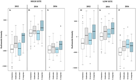
Figure 4.
Comparison of radiometric intensities for A. fraseriana, B. attenuata, B. menziesii and E. marginata species mapped in the high (a–c) and low (d–f) sites for 2012, 2014 and 2016.
3.2.2. Change Detection
Change detection images were generated using the following RBNDVI imagery pairs: 2012/2014, 2014/2015 and 2015/2016 (Figure 5A–C). The colour ramp applied to the imagery specifies blue regions as indicative of increased tree vigour, while red regions highlight areas of stress and dark red of tree death, with neutral colours indicating minimal change.
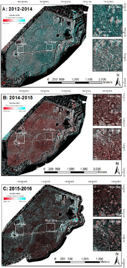
Figure 5.
Composite change images for (A) 2012–2014, (B) 2014–2015 and (C) 2015–2016. Blue regions are indicative of increased tree vigour, while red regions highlight areas of stress and dark red of tree death. Neutral colours indicate minimal change.
The 2012–2014 image (Figure 5A) shows strong growth across the park, following above-average winter rainfall events in 2013–2014 (Figure 2A,B). The 2014–15 composite image (Figure 5B) shows significant stress, which continues to 2015–2016 (Figure 5C) following a > 6 °C weekly temperature increase from the base monthly average (Figure 2C) and below-average rainfall in the 2015 winter season (Figure 2B).
Using the 2012 imagery as a baseline for change detection, change detection images representing a three-year (2012–2015, Figure 6b) and four-year (2012–2016, Figure 6c) period were generated. While some of these pairs do not directly align and some minor edge/shadow effects are present, gross crown condition changes over the long term are evident in both the high and the low sites. A general trend of increasing tree stress is evident from 2014 to 2015 and again to 2016. Stress has been relatively constant at the low site across the four-year period, whereas the high site, which initially exhibited a lower degree of stress in 2012–2014, shows increasing stress (corresponding to a decrease in RBNDVI) in more recent years.
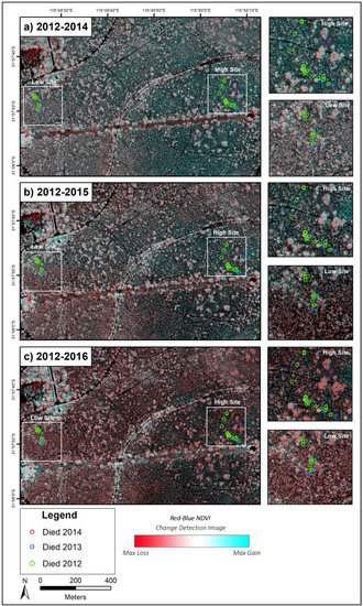
Figure 6.
Composite change images based on the RBNDVI index across a two-year ((a) 2012/2014), three-year ((b) 2012/2015) and four-year ((c) 2012/2016) timeframe, with the colour scale indicating negative change (red—potential tree deaths or high stress), no change (white) and net gain (blue).
4. Discussion
This study merged field and remotely sensed data to monitor vegetation decline (at a park-scale and at a species level) in a coastal woodland subject to multiple, potentially interacting biotic and abiotic stressors (Table 1).
Field-based data collection provided information relating to specific tree species within the nominated study sites, as well as trends in canopy survival and mortality events. This field data provided context for extraction of tree crown spectral characteristics (i.e., relating these to specific species and patterns of stress in subsequent years) and for interpretation of change detection imagery (i.e., relating observed periods of stress and decline in the spectral image to field observations of tree canopy cover and broad mortality events). The combination of field-scale observations and aerial multispectral remote sensing incorporated into a GIS is powerful for not only understanding overall trends in coastal woodlands but also for understanding species-specific responses over a period of time.
4.1. Evalution of Spatial Methods for Monitoring Vegetation Decline
This paper has evaluated the way in which high-spatial resolution airborne multispectral imagery can be used to monitor and detect changes in a coastal woodland over both the short-and long-term [4,13,39]. Based on visual assessment, the RBNDVI metric selected for analysis in this study was considered to most clearly accentuate the tree canopy in comparison to ten other indices (Table 5) commonly used in vegetation studies. Vegetation indices such as the simple ratio or PCD and normalised indices (for example, NDVI) focus on the near-infrared and red bands [70] and are good measures of vegetation health [71]. The RBNDVI index [61] is similar; however, it also incorporates the blue band, which is related to soil properties and reflectance. In the sandy surficial soils of the Swan Coastal Plain, the light colour is responsive in the blue band as a whitening or bleaching signature. This may accentuate the plant and non-plant (i.e., soil) through the differential within RBNDVI and thus provide the best option for delineating tree canopies and for tracking tree mortality events. Qiu et al. [72] suggests the finding of the RBNDVI index being more sensitive for this application than traditional NDVI.
Mapping of individuals using the eCognition Essentials software was largely unsuccessful in this study due to high density clustering of trees within the study sites and across the park, generally. Although impractical on the scale of hectares, manual digitisation of generated geo-objects to ”declump” trees is a feasible option [68]. Even so, the manual separation of tree canopies is challenging, especially in regions of localised growth of one particular species (such as the low site in this study). Use of a region-growing algorithm, an iterative optimisation process which segments imagery based on similar spatial patterns [73], might be a potential option to overcome this limitation. However, the interconnected nature of the canopies and irregular-shaped canopy extent extracted using GEOBIA mean that these methods are unlikely to succeed. Another alternative may be to use higher resolution imagery (such as drone imagery [74]) and digital surface models of canopies [75] to support segmentation of individual species in areas where tree crowns are not spatially discrete. The application of paired change detection images using the RBNDVI imagery demonstrates the capability of multitemporal multispectral imagery in highlighting changes in vegetative cover and stress patterns over time.
Overall, this study found that with application of an appropriate index to delineate tree canopy, vegetation could be mapped and monitored. Tracking of individual trees through time using a GEOBIA approach is limited in woodlands with interconnected canopies, but is possible (albeit to a limited spatial extent) with manual digitisation methods.
4.2. Patterns and Drivers of Tree Decline
Using field and spatial techniques, this study provides new insight into patterns and drivers of tree decline within the Kings Park woodland.
Crosti et al. [9] suggested that the decline of Banksia species in Kings Park was unlikely to be driven by changes in climate (despite the 15% reduction in precipitation from 1939–1999, the time period over which vegetation was monitored) and instead attributed changes in ecosystem health and structure to weed invasion, biotic interactions and fire regime. It is unlikely that weed invasion is driving tree decline over the period of monitoring (2012–2016), as park management has implemented a robust weed eradication scheme across 80 ha of the park [26].
Additionally, while insect and pathogen infection has been identified elsewhere as a potential driver of tree decline [19,76], visual inspection of the study site suggests insect and pathogen infection are not considered to be the likely causes of the patterns of woodland decline (and recovery) at this site.
On the other hand, patterns of stress (Figure 5A–C) appear to be exacerbated after periods of below-average winter rainfall and alleviated after significant rainfall events (refer to Figure 2A and Figure 3B). The dry winters of 2009 and 2010, coupled with elevated summer temperatures in 2009, 2010 and 2011 between 4–6 °C above the average monthly temperatures (Figure 2C) are associated with the greatest occurrence of tree mortality in the park (Table 7). Other studies conducted within the southwest of Western Australia (SWWA) [1,8,51,77,78] have also linked tree mortality in 2011 to this period of sustained drought and heat. Following the combined drought/heat event of 2009/2010/2011, the above average winter rainfall in 2011 and 2013 (Figure 2A), coupled with summer storms in late-2011 and early-2013 (Figure 2B), likely recharged the vadose zone and water table, with the recovery of trees in 2014 indicative of this process. This is evident in overall positive colour reflectance change within the radiometrically-balanced imagery from 2012–2014 (Figure 5A), visually dominated by the processes of undergrowth response within the imagery across the study period from dry to wet.
Trees in the high site have no access to permanent water (~50 m to groundwater) but can access stored moisture within shallow clay lenses at depths of 6–8 m. These trees exhibited more severe stress patterns than trees in the low elevation site (where the groundwater table is around 9–20 meters below ground level) for 2012 and 2016; however, they displayed increased vigour in 2014 following the above-average 2013 winter rainfall. A similar trend was observed in the Rockingham Lakes Regional Park, where Matusick et al. [1] found extensive crown dieback more pronounced at higher elevations, where trees were unable to access the groundwater table and where recharge was ineffective. Similarly, Smettem and Callow [79] and Smettem et al. [80] noted that forest ecosystems of Southwestern Australia were mining groundwater to maintain ecosystem function, with the implication that in more water-deficient sites (e.g., the high site), the ecosystem is less resilient to drought and extreme heat stress.
This is particularly relevant for the isohydric Banksia species, which have a limited water potential range and, therefore, reduced ability to tolerate drought conditions [9,28]. Higher mortality rates were recorded for B. menziesii and B. attenuata in the high site (where subsurface and groundwater resources are limited) (Table 7), and stress patterns for B. menziesii were more pronounced in the high site in 2016 compared to the low site (p < 0.001) (Figure 4 and Table 10).
Despite greater access to the groundwater table, tree mortality in the low site is still significant and may be attributed to the high density of trees within this site—suggesting that competition for resources is a secondary driver of decline in the site when precipitation is inadequate. At this site, the reduced competition for water resources after the 2011 mortality event, in combination with subsequent good rainfall years, is another potential explanation for increased tree vigour observed in 2014. Fire as a driver of tree mortality has been extensively documented in the past, with the wildfire of 1988/1989 linked to largescale tree mortality [15,25]. On the other hand, the work of other authors [24,25] points to the significance of fire as a means of encouraging new seedlings and maintaining overall ecosystem health. However, the ad hoc nature of fires in Kings Park makes it difficult to determine the exact role of fire within the woodland. Monitoring of fire regime, plant competition and plant succession over longer periods will be critical, with the methods applied in this research offering potential tools to evaluate this question as a sufficiently longer-term dataset becomes available.
As recognised by Allen et al. [10], trees are subject to a number of interacting factors, often making it difficult to ascertain a specific driver of mortality. Yet, patterns of mortality in the park suggest that the changing climate, and associated heat and drought events, is the primary driver of tree mortality within the park, with competition between tree species and access to the groundwater table functioning as secondary drivers of tree decline in the low and high sites, respectively.
4.3. Conclusions and Recommendations
This study reported on the ability to monitor and assess spatiotemporal trends of individual trees within a coastal woodland and to assess potential drivers of decline using a combination of field-based monitoring and remote sensing techniques. Selection of the vegetation index RBNDVI allowed individual trees to be mapped in the project study area. This approach was then used to look at change detection and extraction of individual plant-specific radiometric features as a powerful tool for analysing park- and plant-scale trends and patterns of decline.
Within our study site and with the available dataset and based on the RBNDVI index, the application of GEOBIA was of limited benefit in mapping the location of individual trees within a closed-canopy ecosystem (low site). The use of alternative methods, including a region-growing algorithm or higher resolution imagery, may support segmentation of individual species in areas where tree crowns are not spatially discrete. Manual digitisation methods (which were used in this study) are effective, however, not feasible for larger-scale analysis of woodland decline.
In addition to techniques employed in this study, higher resolution monitoring of regions exhibiting increased stress could be undertaken using an unmanned aerial vehicle (UAV), though this is not as suitable for application to the park-scale ecosystem (267 ha). Acquisition of thermal imagery to assess the extent of tree water stress [81] could simultaneously be undertaken using the approach of Berni et al. [42]. These approaches may enable species-specific monitoring to be conducted remotely and provide information regarding periods when vegetation water stress is at a peak. The use of drone multispectral sensors could also allow for a broader range of indices to be calculated at the specific tree level [42], potentially increasing the ability to map tree health and presence/absence from the imagery. As part of monitoring the ecosystem structure, it may also be beneficial to undertake field-based and, where possible, remotely sensed monitoring of seedling survival within the woodland. Competition with surrounding shrubbery and established trees [25] may lead to low survival rates of seedlings and, thus, have implications for diversity of trees and ecosystem changes. Collection of ground radiometric data, specifically of vegetation or radiometrically similar reference targets at the time of overflight, would improve the uncertainty in using invariant targets, though cannot be applied retrospectively to long time-series datasets collected before studies started, such as was the approach in this study, particularly where imagery is collected and processed by a commercial operation and used opportunistically in a study.
Secondary drivers of decline (such as competition and lower groundwater levels, as identified in this study) are known to exacerbate existing patterns of stress in vegetation, and management of these secondary drivers is therefore critical. The Kings Park management have been proactive in containing the spread of weeds (especially, Ehrharta calycina) [26], harvesting stormwater during winter to minimise reliance on groundwater for irrigation and improving irrigation systems and infrastructure to reduce incidental water loss. Crown thinning to reduce competition between tree species [10] and developing a fire regime that promotes reseeding and resprouting of trees, but which does not result in the mortality of established trees [25], are additional strategies to minimise the impact of secondary drivers of tree decline. A project investigating the impacts of fire on native species richness and composition in Kings Park is currently underway, with the first prescribed burn undertaken in 2015 and monitoring of impacts ongoing [82]. Managing the effects of a changing climate is more complex due to the unpredictability of the timing and severity of extreme climate events. Depletion of carbohydrate reserves due to increased winter temperatures may have implications for carbon starvation thresholds in trees [10]; however, this is highly dependent on the tree species.
Monitoring vegetation health on a continual basis and observing the response of biota to changes in climate and undertaking field-based research into species survival mechanisms under high-stress conditions (e.g., when water is scarce) will inform management response to the implementation of appropriate adaptation strategies [8].
Author Contributions
R.-A.B. and J.N.C. conceptualised the study and methodology. R.-A.B. led the data collection with support from J.N.C. and others (see acknowledgements). R.-A.B. led the spatial and statistical analysis with support and supervision from J.N.C. R.-A.B. led the writing and drafting of the majority of figures, with J.N.C. producing others and providing editorial support to the writing process. All authors have read and agreed to the published version of the manuscript.
Funding
This project was supported by the Australian Government through the Australian Research Council’s Linkage Projects funding scheme (project LP140100736), in partnership with the Botanic Gardens and Parks Authority (now Department of Biodiversity Conservation and Attractions) and SpecTerra Systems Pty Ltd. The views expressed herein are those of the authors and not necessarily those of the Australian Government or Australian Research Council.
Acknowledgments
The authors would like to acknowledge Anthea Challis for her assistance conducting fieldwork and Ben Miller and Jason Stevens (Botanic Gardens and Parks Authority) for input and initial site logistics planning.
Conflicts of Interest
The authors declare no conflicts of interest.
References
- Matusick, G.; Ruthrof, K.X.; Hardy, G. Drought and heat triggers sudden and severe dieback in a dominant Mediterranean-type woodland species. Open J. For. 2012, 2, 183–186. [Google Scholar] [CrossRef]
- Hughes, L. Climate change and Australia: Key vulnerable regions. Reg. Environ. Chang. 2011, 11, 189–195. [Google Scholar] [CrossRef]
- Ramalho, C.E.; Laliberté, E.; Poot, P.; Hobbs, R.J. Complex effects of fragmentation on remnant woodland plant communities of a rapidly urbanizing biodiversity hotspot. Ecol. Soc. Am. 2014, 95, 2466–2478. [Google Scholar] [CrossRef]
- Lawley, V.; Lewis, M.; Clarke, K.; Ostendorf, B. Site-based and remote sensing methods for monitoring indicators of vegetation condition: An Australian review. Ecol. Indic. 2016, 60, 1273–1283. [Google Scholar] [CrossRef]
- Seto, K.C.; Güneralp, B.; Hutyra, L.R. Global forecasts of urban expansion to 2030 and direct impacts on biodiversity and carbon pools. Proc. Natl. Acad. Sci. USA 2012, 109, 16083–16088. [Google Scholar] [CrossRef]
- Australian Bureau of Statistics. 3218.0—Regional Population Growth, Australia, 2017–2018. Available online: https://www.abs.gov.au/ausstats/abs@.nsf/Latestproducts/3218.0Main%20Features402017-18?opendocument&tabname=Summary&prodno=3218.0&issue=2017-18&num=&view (accessed on 4 April 2016).
- Beard, J.S. Natural woodland in King’s Park, Perth. West. Aust. Nat. 1967, 10, 77–84. [Google Scholar]
- Brouwers, N.; Matusick, G.; Ruthrof, K.; Lyons, T.; Hardy, G. Landscape-scale assessment of tree crown dieback following extreme drought and heat in a Mediterranean eucalypt forest ecosystem. Landsc. Ecol. 2013, 28, 69–80. [Google Scholar] [CrossRef]
- Crosti, R.; Dixon, K.W.; Ladd, P.G.; Yates, C.J. Changes in the structure and species dominance in vegetation over 60 years in an urban bushland remnant. Pac. Conserv. Biol. 2007, 13, 158–170. [Google Scholar] [CrossRef]
- Allen, C.D.; Macalady, A.K.; Chenchouni, H.; Bachelet, H.; McDowell, N.; Venetier, M.; Kitzberger, T.; Rigling, A.; Breshears, D.D.; Hogg, E.H.; et al. A global overview of drought and heat-induced tree mortality reveals emerging climate change risks for forests. For. Ecol. Manag. 2010, 259, 660–684. [Google Scholar] [CrossRef]
- Brouwers, N.C.; Mercer, J.; Lyons, T.; Poot, P.; Veneklaas, E.; Hardy, G. Climate and landscape drivers of tree decline in a Mediterranean region. Ecol. Evol. 2013, 3, 67–79. [Google Scholar] [CrossRef]
- McDowell, N.; Pockman, W.T.; Allen, C.D.; Breshears, D.D.; Cobb, N.; Kolb, T.; Plaut, J.; Sperry, J.; West, A.; Williams, D.G.; et al. Mechanisms of plant survival and mortality during drought: Why do some plants survive while others succumb to drought? New Phytol. 2008, 178, 719–739. [Google Scholar] [CrossRef] [PubMed]
- Moore, C.E.; Brown, T.; Keenan, T.F.; Duursma, R.A.; van Dijk, A.I.J.M.; Beringer, J.; Culvenor, D.; Evans, B.; Huete, A.; Hutley, L.B.; et al. Reviews and syntheses: Australian vegetation phenology: New insights from satellite remote sensing and digital repeat photography. Biogeosciences 2016, 13, 5085–5102. [Google Scholar] [CrossRef]
- Baird, A.M. Regeneration after fire in King’s Park, Perth, Western Australia. J. R. Soc. West. Aust. 1977, 60, 1–22. [Google Scholar]
- Bell, D.T.; Loneragan, W.A.; Ridley, W.J.; Dixon, K.W.; Dixon, I.R. Response of tree canopy species of Kings Park, Perth, Western Australia to the severe summer wildfire of January 1989. J. R. Soc. West. Aust. 1992, 75, 35–40. [Google Scholar]
- Briant, G.; Valery, G.; Laurance, S.G.W. Habitat fragmentation and the desiccation of forest canopies: A case study from eastern Amazonia. Biol. Conserv. 2010, 143, 2763–2769. [Google Scholar] [CrossRef]
- Threatened Species Scientific Committee. Approved Conservation Advice (Incorporating Listing Advice) for the Banksia Woodlands of the Swan Coastal Plain Ecological Community; Department of the Environment and Energy: Canberra, Australia, 2016.
- Keenan, T.F.; Darby, B.; Felts, E.; Sonnentag, O.; Friedl, M.A.; Hufkens, K.; O’Keefe, J.; Klosterman, S.; Munger, J.W.; Toomey, M.; et al. Tracking forest phenology and seasonal physiology using digital repeat photography: A critical assessment. Ecol. Appl. 2014, 24, 1478–1489. [Google Scholar] [CrossRef]
- Shearer, B.L.; Crane, C.E.; Barrett, S.; Cochrane, A. Phytophthora cinnamomi invasion, a major threatening process to conservation of flora diversity in the South-west Botanical Province of Western Australia. Aust. J. Bot. 2007, 55, 225–238. [Google Scholar] [CrossRef]
- Altmann, S.H. Crown condition, water availability, insect damage and landscape features: Are they important to the Chilean tree Nothofagus glauca (Northofagaceae) in the context of climate change? Aust. J. Bot. 2013, 61, 394–403. [Google Scholar] [CrossRef]
- Bennett, E.M. The Bushland Plants of Kings Park, Western Australia; Kings Park Board: Kings Park, Australia, 1988.
- Fisher, J.L.; Veneklaas, E.J.; Lambers, H.; Loneragan, W.A. Enhanced soil and leaf nutrient status of a Western Australian Banksia woodland community invaded by Ehraharta calycina and Pelargonium capitatum. Plant Soil 2006, 284, 253–264. [Google Scholar] [CrossRef]
- Catford, J.A.; Daehler, C.C.; Murphy, H.T.; Sheppard, A.W.; Hardesty, B.D.; Westcott, D.A.; Rejmanek, M.; Bellingham, P.J.; Pergl, J.; Horvitz, C.C.; et al. The intermediate disturbance hypothesis and plant invasions: Implications for species richness and management. Perspect. Plant Ecol. Evol. Syst. 2012, 14, 231–241. [Google Scholar] [CrossRef]
- Close, D.C.; Davidson, N.J.; Swanborough, P.W. Fire history and understorey vegetation: Water and nutrient relations of Eucalyptus gomphocephala and E. delegatensis overstorey trees. For. Ecol. Manag. 2011, 262, 208–214. [Google Scholar] [CrossRef]
- Bell, D.T. Ecological response syndromes in the flora of Southwestern Western Australia: Fire resprouters versus reseeders. Bot. Rev. 2001, 67, 417–440. [Google Scholar] [CrossRef]
- Botanic Gardens and Parks Authority. 2014-15 Annual Report; Botanic Gardens and Parks Authorit: Kings Park, Australia, 2016.
- Evans, B.J.; Lyons, T. Bioclimatic Extremes Drive Forest Mortality in Southwest, Western Australia. Climate 2013, 1, 28–52. [Google Scholar] [CrossRef]
- Canham, C.A.; Froend, R.H.; Stock, W.D. Water stress vulnerability of four Banksia species in contrasting ecohydrological habitats on the Gnangara Mound, Western Australia. Plant Cell Environ. 2009, 32, 64–72. [Google Scholar] [CrossRef]
- Poot, P.; Veneklaas, E.J. Species distribution and crown decline are associated with contrasting water relations in four common sympatric eucalypt species in southwestern Australia. Plant Soil 2013, 364, 409–423. [Google Scholar] [CrossRef]
- Kinal, J.; Stoneman, G.L. Disconnection of groundwater from surface water causes a fundamental change in hydrology in a forested catchment in south-western Australia. J. Hydrol. 2012, 472–473, 14–24. [Google Scholar] [CrossRef]
- Mandre, M.; Kiviste, A.; Köster, K. Environmental stress and forest ecosystem. For. Ecol. Manag. 2011, 2621, 53–55. [Google Scholar] [CrossRef]
- Dale, V.H.; Joyce, L.A.; McNulty, S.; Neilson, R.P. The interplay between climate change, forests and disturbances. Sci. Total Environ. 2000, 262, 201–204. [Google Scholar] [CrossRef]
- Ceccato, P.; Flasse, S.; Tarantola, S.; Jacquemoud, S.; Gregoire, J. Detecting vegetation leaf water content using reflectance in the optical domain. Remote Sens. Environ. 2001, 77, 22–33. [Google Scholar] [CrossRef]
- Groom, P.K.; Froend, R.H.; Mattiske, E.M.; Gurner, R.P. Long-term changes in vigour and distribution of Banksia and Melaleuca overstorey species on the Swan Coastal Plain. J. R. Soc. West. Aust. 2001, 84, 63–69. [Google Scholar]
- Harris, A.; Bryant, R.G.; Baird, A.J. Mapping the effects of water stress on Sphagnum: Preliminary observations using airborne remote sensing. Remote Sens. Environ. 2006, 100, 363–378. [Google Scholar] [CrossRef]
- Xie, Y.; Sha, Z.; Yu, M. Remote sensing imagery in vegetation mapping: A review. J. Plant Ecol. 2008, 1, 9–23. [Google Scholar] [CrossRef]
- Tucker, C.J. Red and photographic infrared linear combinations for monitoring vegetation. Remote Sens. Environ. 1979, 8, 127–150. [Google Scholar] [CrossRef]
- Toomey, M.; Friedl, M.A.; Frolking, S.; Hutkens, K.; Klosterman, S.; Sonnentag, O.; Al, B.D.D.E. Greenness indices from digital cameras predict the timing and seasonal dynamics of canopy-scale photosynthesis. Ecol. Appl. 2015, 1, 99–115. [Google Scholar] [CrossRef]
- Brundrett, M.; van Dongen, R.; Huntley, B.; Tay, N.; Longman, V. A monitoring toolkit for banksia woodlands: Comparison of different scale methods to measure recovery of vegetation after fire. Remote Sens. Ecol. Conserv. 2018, 5, 33–54. [Google Scholar] [CrossRef]
- Bréda, N.; Granier, A.; Aussenac, G. Effects of thinning on soil and tree water relations, transpiration and growth in an oak forest (Quercus petraea (Matt.) Liebl.). Tree Physiol. 1995, 15, 295–306. [Google Scholar]
- Smith, D.M.; Allen, S.J. Measurement of sap flow in plant stems. J. Exp. Bot. 1996, 47, 1833–1844. [Google Scholar] [CrossRef]
- Berni, J.A.J.; Zarco-Tejada, P.J.; Gonzalez-Dugo, V.; Fereres, E. Remote sensing of thermal water stress indicators in peach. Acta Hortic. 2012, 962, 325–332. [Google Scholar] [CrossRef]
- Boulet, G.; Mougenot, B.; Abdelouahab, T.B. An evaporation test based on Thermal Infra Red remote-sensing to select appropriate soil hydraulic properties. J. Hydrol. 2009, 376, 589–598. [Google Scholar] [CrossRef]
- Barton, C.V.M. Advances in remote sensing of plant stress. Plant Soil 2012, 354, 41–44. [Google Scholar] [CrossRef]
- Yates, C.J.; Hopper, S.D.; Taplin, R.H. Native insect flower visitor diversity and feral honeybees on jarrah (Eucalyptus marginata) in Kings Park, an urban bushland remnant. J. R. Soc. West. Aust. 2005, 88, 147–153. [Google Scholar]
- Keighery, G. Banksia woodlands: A Perth Icon. In Perth Banksia Woodlands, Precious and under Threat, Proceedings of a Symposium on the Ecology of These Ancient Woodlands and Their Need for Protection from Neglect and Destruction; Sarti, K., Ed.; Urban Bushland Council: West Perth, Australia, 2011; pp. 3–10. [Google Scholar]
- Challis, A.; Stevens, J.C.; McGrath, G.; Miller, B.P. Plant and environmental factors associated with drought-induced mortality in two facultative phreatophytic trees. Plant Soil 2016, 404, 1–16. [Google Scholar] [CrossRef]
- Bureau of Meteorology. Cimate Data Online. Available online: http://www.bom.gov.au/climate/data/ (accessed on 4 April 2016).
- Challis, A.J. Mortality Patterns and Physiological Responses of the Canopy Tree, Banksia Menziesii in Relation to Varying Summer Water Availability in an Urban Remnant. Honours Thesis, The University of Western Australia, Crawley, Australia, 2014. [Google Scholar]
- Lee, M.T.; Peet, R.K.; Roberts, S.D.; Wentworth, T.R. CVS-EEP Protocol for Recording Vegetation. Available online: http://cvs.bio.unc.edu/protocol/cvs-eep-protocol-v4.2-lev1-5.pdf (accessed on 18 February 2020).
- Wallace, J.F.; Canci, M.; Wu, X.; Baddeley, A. Monitoring native vegetation on an urban groundwater supply mound using airborne digital imagery. Spat. Sci. 2008, 53, 63–73. [Google Scholar] [CrossRef]
- Uribeetxebarria, A.; Daniele, E.; Escolà, A.; Arnó, J.; Martínez-Casasnovas, J.A. Spatial variability in orchards after land transformation: Consequences for precision agriculture practices. Sci. Total Environ. 2018, 635, 343–352. [Google Scholar] [CrossRef]
- Nielsen, A.A.; Conradsen, K.; Simpson, J.J. Multivariate Alteration Detection (MAD) and MAF Postprocessing in Multispectral, Bitemporal Image Data: New Approaches to Change Detection Studies. Remote Sens. Environ. 1998, 64, 1–19. [Google Scholar] [CrossRef]
- Furby, S.L.; Campbell, N.A. Calibrating images from different dates to ‘like-value’ digital counts. Remote Sens. Environ. 2001, 77, 186–196. [Google Scholar] [CrossRef]
- Nash, J.E.; Sutcliffe, J.V. River flow forecasting through conceptual models part 1—A discussion of principles. J. Hydrol. 1970, 10, 282–290. [Google Scholar] [CrossRef]
- Willmott, C.J. On the validation of models. Phys. Geogr. 1981, 2, 184–194. [Google Scholar] [CrossRef]
- Fitzgerald, G.J.; Perry, E.M.; Flower, K.C.; Callow, J.N.; Boruff, B.; Delahunty, A.; Wallace, A.; Nuttall, J. Frost Damage Assessment in Wheat Using Spectral Mixture Analysis. Remote Sens. 2019, 11, 2476. [Google Scholar] [CrossRef]
- Xue, J.; Su, B. Significant remote sensing vegetation indices: A review of developments and applications. J. Sens. 2017, 2017, 1–17. [Google Scholar] [CrossRef]
- Huete, A.; Didan, K.; Miura, T.; Rodriguez, E.P.; Gao, X.; Ferreira, L.G. Overview of the radiometric and biophysical performance of the MODIS vegetation indices. Remote Sens. Environ. 2002, 83, 195–213. [Google Scholar] [CrossRef]
- Rondeaux, G.; Steven, M.; Baret, F. Optimization of soil-adjusted vegetation indices. Remote Sens. Environ. 1996, 55, 95–107. [Google Scholar] [CrossRef]
- Wang, F.; Huang, J.; Tang, Y.; Wang, X. New vegetation index and its application in estimating leaf area index of rice. Rice Sci. 2007, 14, 195–2013. [Google Scholar] [CrossRef]
- Vincini, M.; Frazzi, E.; D’Allessio, P. A broad-band leaf chlorophyll vegetation index at the canopy scale. Precis. Agric. 2008, 9, 303–319. [Google Scholar] [CrossRef]
- Motohka, T.; Nasahara, K.N.; Oguma, H.; Tsuchida, S. Applicability of green-red vegetation index for remote sensing of vegetation phenology. Remote Sens. 2010, 2, 2369–2387. [Google Scholar] [CrossRef]
- Wu, C.; Niu, Z.; Gao, S. The potential of the satellite derived green chlorophyll index for estimating midday light use efficiency in maize, coniferous forest and grassland. Ecol. Indic. 2012, 14, 66–73. [Google Scholar] [CrossRef]
- Gitelson, A.A.; Kaufman, Y.J.; Merzlyak, M.N. Use of a green channel in remote sensing of global vegetation from EOS-MODIS. Remote Sens. Environ. 1996, 58, 289–298. [Google Scholar] [CrossRef]
- Glenn, E.P.; Huete, A.R.; Nagler, P.L.; Nelson, S.G. Relationship between remotely-sensed vegetation indices, canopy attributes and plant physiological processes: What vegetation indices can and cannot tell us about the landscape. Sensors 2008, 8, 2136–2160. [Google Scholar] [CrossRef]
- Blaschke, T. Object based image analysis for remote sensing. ISPRS J. Photogramm. Remote Sens. 2010, 65, 2–16. [Google Scholar] [CrossRef]
- Chang, Y.; Baddeley, A.; Wallace, J.F.; Canci, M. Spatial statistical analysis of tree deaths using airborne digital imagery. Int. J. Appl. Earth Obs. Geoinf. 2013, 21, 418–426. [Google Scholar] [CrossRef]
- Johansen, K.; Arroyo, L.A.; Phinn, S.; Witte, C. Comparison of geo-object based and pixel-based change detection of riparian environments using high spatial resolution multi-spectral imagery. Photogramm. Eng. Remote Sens. 2010, 76, 123–136. [Google Scholar] [CrossRef]
- Reid, S.L.; Walker, J.L.; Schaaf, A. Using multi-spectral landsat imagery to examine forest health trends at Fort Benning, Georgia. In Proceedings of the 18th Biennial Southern Silvicultural Research Conference, Knoxville, TN, USA, 2–5 March 2016. [Google Scholar]
- Bokusheva, R.; Kogan, F.; Vitkovskaya, I.; Conradt, S.; Batyrbayeva, M. Satellite-based vegetation health indices as a criteria for insuring against drought-related yield losses. Agric. For. Meteorol. 2016, 220, 200–206. [Google Scholar] [CrossRef]
- Qiu, C.; Liao, G.; Tang, H.; Liu, F.; Liao, X.; Zhang, R.; Zhao, Z. Derivative Parameters of Hyperspectral NDVI and Its Application in the Inversion of Rapeseed Leaf Area Index. Appl. Sci. 2018, 8, 1300. [Google Scholar] [CrossRef]
- Jellema, A.; Stobbelaar, D.; Goroot, J.C.J.; Rossing, W.A.H. Landscape character assessment using region growing techniques in geographical information systems. J. Environ. Manag. 2009, 90, 5161–5174. [Google Scholar] [CrossRef] [PubMed]
- Chen, G.; Weng, Q.; Hay, G.J.; He, Y. Geographic Object-based Image Analysis (GEOBIA): Emerging trends and future opportunities. Gisci. Remote Sens. 2018, 55, 159–182. [Google Scholar] [CrossRef]
- Godwin, C.; Chen, G.; Singh, K.K. The impact of urban residential development patterns on forestcarbon density: An integration of LiDAR, aerial photography and field mensuration. Landsc. Urban Plan. 2015, 136, 97–109. [Google Scholar] [CrossRef]
- Keith, H.; van Gorsel, E.; Jacobsen, K.L.; Cleugh, H.A. Dynamics of carbon exchange in a Eucalyptus forest in response to interacting disturbance factors. Agric. For. Meteorol. 2012, 153, 67–81. [Google Scholar] [CrossRef]
- Bader, M.K.F.; Ehrenberger, W.; Bitter, R.; Stevens, J.; Miller, B.P.; Chopard, J.; Ruger, S.; Hardy, G.E.S.J.; Poot, P.; Dixon, K.W.; et al. Spatio-temporal water dynamics in mature Banksia menziesii trees during drought. Physiol. Plant. 2014, 152, 301–315. [Google Scholar] [CrossRef]
- Evans, B.; Lyons, T.J.; Barber, P.A.; Stone, C.; Hardy, G. Detecting Change in Vegetation Condition using High Resolution Digital Multispectral Imagery. In Proceedings of the 34th International Symposium on Remote Sensing of Environment—The GEOSS Era: Towards Operational Environmental Monitoring, Sydney, Australia, 10–15 April 2011; pp. 1–5. [Google Scholar]
- Smettem, K.; Callow, N. Impact of forest cover and aridity on the interplay between effective rooting depth and annual runoff in South-Western Australia. Water 2014, 6, 2539–2551. [Google Scholar] [CrossRef]
- Smettem, K.R.J.; Waring, R.H.; Callow, J.N.; Wilson, M.; Mu, Q. Satellite-derived estimates of forest leaf area index in southwest Western Australia are not tightly coupled to interannual variations in rainfall: Implications for groundwater decline in a drying climate. Glob. Chang. Biol. 2013, 19, 2401–2412. [Google Scholar] [CrossRef]
- Jones, H.G.; Serrai, R.; Loveys, B.R.; Xiong, L.; Wheaton, A.; Price, A.H. Thermal infrared imaging of crop canopies for the remote diagnosis and quantification of plant responses to water stress in the field. Funct. Plant Biol. 2009, 36, 978–989. [Google Scholar] [CrossRef]
- Botanic Gardens and Parks Authority. Fire Risk Management. Available online: https://www.bgpa.wa.gov.au/about-us/information/research/ecosystem-ecology/fire-risk-management (accessed on 29 October 2019).
© 2020 by the authors. Licensee MDPI, Basel, Switzerland. This article is an open access article distributed under the terms and conditions of the Creative Commons Attribution (CC BY) license (http://creativecommons.org/licenses/by/4.0/).