Article

Evaluation of Multi-Satellite Precipitation Datasets and Their Error Propagation in Hydrological Modeling in a Monsoon-Prone Region

1
State Key Laboratory of Water Resources and Hydropower Engineering Science, Wuhan University, Wuhan 430072, China
2
Hubei Key Laboratory of Water System Science for Sponge City Construction, Wuhan University, Wuhan 430072, China
3
NORCE Norwegian Research Centre, Bjerknes Centre for Climate Research, Jahnebakken 5, NO-5007 Bergen, Norway
4
Department of Geosciences, University of Oslo, Sem Saelands vei 1, P.O. Box 1047, Blindern, NO-0316 Oslo, Norway
*
Author to whom correspondence should be addressed.
Remote Sens. 2020, 12(21), 3550; https://doi.org/10.3390/rs12213550
Submission received: 13 September 2020 / Revised: 25 October 2020 / Accepted: 26 October 2020 / Published: 30 October 2020
(This article belongs to the Special Issue Remote Sensing of Hydro-Meteorology)

Abstract

:
This study comprehensively evaluates eight satellite-based precipitation datasets in streamflow simulations on a monsoon-climate watershed in China. Two mutually independent datasets—one dense-gauge and one gauge-interpolated dataset—are used as references because commonly used gauge-interpolated datasets may be biased and unable to reflect the real performance of satellite-based precipitation due to sparse networks. The dense-gauge dataset includes a substantial number of gauges, which can better represent the spatial variability of precipitation. Eight satellite-based precipitation datasets include two raw satellite datasets, Precipitation Estimation from Remotely Sensed Information using Artificial Neural Networks (PERSIANN) and Climate Prediction Center MORPHing raw satellite dataset (CMORPH RAW); four satellite-gauge datasets, Tropical Rainfall Measuring Mission 3B42 (TRMM), PERSIANN Climate Data Record (PERSIANN CDR), CMORPH bias-corrected (CMORPH CRT), and gauge blended datasets (CMORPH BLD); and two satellite-reanalysis-gauge datasets, Multi-Source Weighted-Ensemble Precipitation (MSWEP) and Climate Hazards Group InfraRed Precipitation with Stations (CHIRPS). The uncertainty related to hydrologic model physics is investigated using two different hydrological models. A set of statistical indices is utilized to comprehensively evaluate the precipitation datasets from different perspectives, including detection, systematic, random errors, and precision for simulating extreme precipitation. Results show that CMORPH BLD and MSWEP generally perform better than other datasets. In terms of hydrological simulations, all satellite-based datasets show significant dampening effects for the random error during the transformation process from precipitation to runoff; however, these effects cannot hold for the systematic error. Even though different hydrological models indeed introduce uncertainties to the simulated hydrological processes, the relative hydrological performance of the satellite-based datasets is consistent in both models. Namely, CMORPH BLD performs the best, which is followed by MSWEP, CMORPH CRT, and TRMM. PERSIANN CDR and CHIRPS perform moderately well, and two raw satellite datasets are not recommended as proxies of gauged observations for their worse performances.

Graphical Abstract

1. Introduction

Precipitation is one of the most important meteorological variables in the hydrologic cycle and is often used as the fundamental input to environmental models for agricultural, meteorological, and hydrological studies [1]. However, precipitation measured by pluviometers usually suffers from many problems, such as sparse station distribution at high altitudes or in rural areas, missing data, and short time periods [2]. Meanwhile, artificial errors in measurements are inevitable [3]. In addition, surface observational networks have indicated decreasing coverages and spatial densities, which may limit the future capacity to measure precipitation for many parts of the world [4,5].
As a proxy for gauged precipitation, gridded precipitation with high spatial and temporal coverage has been developed, which can be generally classified into three categories based on different data sources: (1) gauge-interpolated, (2) reanalysis-based, and (3) satellite-based precipitation [6,7,8,9,10].
Gauge-interpolated precipitation, such as the Global Precipitation Climatology Centre (GPCC) [11] and Climate Research Unit (CRU) [12], is generated by interpolating gauged data to grids with different spatial resolutions [13,14]. Thiessen polygons, Kriging, and inverse distance weighting (IDW) are the most widely used interpolation algorithms [2,15]. More sophisticated interpolation methods take extra geographical or physical information into consideration, such as topography and atmospheric lapse rate [13,14].
Reanalysis-based precipitation is produced by assimilating various observations (e.g., weather stations, satellites, ships, and buoys) into a climate model to generate various meteorological variables with a consistent spatial and temporal resolution [4,16,17,18]. The reliability of reanalysis-based precipitation relies on assimilated observations, climate model parameters, and the interactions between models and observations. Several reanalysis datasets have been made freely available, such as the National Centers for Environmental Prediction/National Center for Atmosphere Research Reanalysis (NCEP/NCAR) [19], the European Centre for Medium-Range Weather Forecasts Reanalysis (ERA) [20], and the NCEP Climate Forest System Reanalysis (CFSR) [21].
Satellite-based precipitation, with a global and continuous temporal scale, estimates precipitation using polar-orbiting passive microwave (PMW) sensors on low-Earth-orbiting satellites and geosynchronous infrared (IR) sensors on geostationary satellites [22,23,24]. PMW sensors could observe the emissions and lower-atmosphere scattering signals of rainfall, snow, and ice contents, while IR sensors indirectly measure the lower-level rainfall rate by collecting cloud-top temperature and cloud height [25]. Usually, in regions with gauges, satellite-based datasets are modified by gauged measurements to offset their limited abilities [26]. Over the past 30 years, a number of precipitation datasets that combine gauges, PMW, and IR data to produce precipitation estimates are available with the spatial resolution on 0.25 latitude/longitude or finer. These include monthly Global Precipitation Climatology Project (GPCP) [27], daily Precipitation Estimation from Remotely Sensed Information Using Artificial Neural Networks (PERSIANN) [28], Tropical Rainfall Measuring Mission (TRMM) Multi-satellite Precipitation Analysis (TMPA) [29], and Global Precipitation Measurement (GPM) [30].
Although gauge-interpolated and reanalysis-based precipitation may be more appropriate for climate change studies for their long-term data records, it is often difficult to verify their reliabilities in regions with sparse weather station networks [31,32]. Satellite-based datasets could estimate precipitation with a global and homogeneous spatial coverage; this spatial continuity could provide valuable information for hydrological modeling, especially for ungauged watersheds. In recent years, a few global-scale studies are revealing that the performances of satellite-based datasets differ regionally and temporally and correlate to topography, seasonality, and climatology [6,23,33,34]. However, the lack of global and sufficiently dense precipitation references makes these results of satellite-based precipitation still unreliable and inadequate for operational purposes, such as flood forecasting [35]. Therefore, a regional ground validation of satellite-based precipitation datasets based on dense gauges references, especially for their hydrological performances, still requires to be conducted [36,37,38,39,40,41,42,43,44]. Although most studies revealed the potential of satellite-based precipitation datasets for hydrological simulations, they also report error sources during the hydrological modeling of satellite-based datasets. Generally, two main sources are (1) the error of the satellite-based datasets and (2) the error propagation of satellite-based datasets through the hydrological model [45].
The monsoon regions, having an obvious seasonal variation of precipitation, have always been a research focus of satellite-based precipitation datasets [46,47,48,49,50,51,52]. For example, Prakash et al. [51] compared four satellite-based precipitation datasets (Climate Prediction Center MORPHing-raw satellite dataset (CMORPH RAW), Naval Research Laboratory (NRL)-blended, PERSIANN, and TRMM 3B42) with the gauged-interpolated dataset in one Indian monsoon region with respect to their abilities to simulate the seasonal rainfall and the rainfall detection abilities over regions with diverse topography. The results show that although all four datasets underestimate the summer seasonal mean rainfall (June to September), TRMM 3B42 generally performs better than the other three datasets mainly due to its incorporation of rain gauge observations. Mou et al. [49] compared five satellite-based precipitation datasets (TRMM 3B42, its real-time dataset TRMM 3B42RT, GPCP-1DD, PERSIANN Climate Data Record (PERSIANN CDR), and CMORPH RAW) and a gauge-interpolated dataset (Asian Precipitation-Highly Resolved Observational Data Integration Towards Evaluation of Water Resources (APHRODITE)) at daily, monthly, seasonal, and annual scales with rain gauges over Malaysia. It was found that TRMM 3B42 and APHRODITE performed the best, while PERSIANN CDR slightly overestimated observed precipitation, and the other three satellite-based datasets showed the worst performance. In addition, all six precipitation datasets show better performances in southern Peninsular Malaysia, which receives higher precipitation, while worse performances appear in the western and dryer Peninsular Malaysia.
There also have been some studies executed in the monsoon regions aiming to evaluate the applicability of satellite-based datasets in hydrologic simulations [53,54,55,56,57,58,59,60]. For example, Tong et al. [58] evaluated four satellite-based datasets (TRMM 3B42, TRMM 3B42RT, CMORPH RAW, and PERSIANN) through comparing with the gauged China Meteorological Administration dataset (CMA) in streamflow simulations over the Tibetan Plateau based on the distributed Variable Infiltration Capacity (VIC) hydrological model. It was found that the error sources of these datasets are systematically different in different seasons. Furthermore, TRMM 3B42 shows comparable performance to CMA for both monthly and daily streamflow simulations due to its monthly gauge adjustment. However, the other three satellite-based datasets only show potentials or little capability for streamflow simulations over TP. In addition, five satellite-based precipitation datasets (TRMM 3B42, TRMM 3B42RT, CMORPH RAW, CMORPH CRT, and CMORPH BLD) were used by Wang et al. [59] to simulate the daily streamflow by driving the distributed Vegetation Interface Processes (VIP) model over two river basins in the southeastern Tibetan Plateau. The results show that these satellite-based datasets perform better in summer than other seasons, and CMORPH BLD performs the best for runoff simulations. TRMM 3B42 and CMORPH CRT show much better performance than their uncorrected counterparts: TRMM 3B42RT and CMORPH RAW.
From the previous studies, we found that first, there are relatively few evaluations focusing on satellite-based precipitation datasets in the monsoon regions of southern China, which is a flood-prone area. Both the flood predictions and water resource management are mainly based on hydrological simulations. Moreover, most existing studies in the monsoon characterized regions only compare several commonly used satellite-based datasets (such as TRMM and CMORPH serial datasets) and some promising recently released precipitation datasets, such as PERSIANN CDR, Climate Hazards Group InfraRed Precipitation with Stations V2.0 (CHIRPS), and Multi-Source Weighted-Ensemble Precipitation V2.0 (MSWEP) have not been thoroughly evaluated. Second, it is crucial to ensure that the gauged benchmark reference is sufficient to reflect the real performance of satellite-based precipitation when testing satellite-based datasets. However, many studies compared the satellite-based datasets based on the sparse-gauge datasets or gridded datasets generating from sparse gauges, which may not accurately reflect the spatial characteristic of precipitation [47,49,54,59,60]. Furthermore, when evaluating the accuracies of satellite-based datasets, the gauged references in some studies are not independent of the satellite-based datasets, which uses the gauged precipitation as part of their source data [49,52,58]. Third, despite the fact that some studies show that the performance of hydrological simulation is highly dependent on the satellite-based datasets themselves in the monsoon regions, the uncertainties of hydrological models caused by different models’ complexities could also influence the hydrological simulation. The impact of these two uncertainties has not been carefully examined.
The latest review article of Maggioni et al. [35] pointed out that one of the future research areas for satellite-based precipitation datasets is to study the conditions (climate type, basin area, acceptable error in the output, and model structure) under which satellite-based precipitation could be successfully used in hydrological models. In order to provide a comprehensive understanding of the error of the satellite-based precipitation and its error propagation through hydrological models for monsoon-characterized watersheds, this study tests the reliability of eight satellite-based precipitation datasets in hydrological modeling for a large-sized (>80,000 km2) monsoon-characterized watershed (Xiangjiang River Basin) in southern China. Even though one of the main usages of the satellite-based datasets is for ungauged watersheds or watersheds with spare weather stations, the test of their reliability requires a watershed with dense gauges. The Xiangjiang River Basin, which has 267 precipitation gauges (referred to as the dense-gauge precipitation dataset in the study), can meet this requirement for an 80,000 km2 surface area. All the eight satellite-based precipitation datasets include TRMM 3B42 (TRMM), PERSIANN, PERSIANN CDR, CMORPH RAW, CMORPH bias-corrected (CMORPH CRT), CMORPH gauge blended (CMORPH BLD), MSWEP, and CHIRPS. In addition to using the dense-gauge precipitation dataset as a reference, an independent gridded gauge-interpolated precipitation dataset is also used, which incorporates much fewer stations from the National Meteorological Information Center dataset from the China Meteorological Administration (CN05) [61]. As high-density gauged precipitation is usually not available in China, CN05 is commonly used for meteorological and hydrological studies over most watersheds [62,63,64]. This study could be extended to test whether CN05 is capable of being used as a reliable reference for using satellite-based datasets over other watersheds where gauges are much less dense. To investigate the uncertainty related to hydrological models, the lumped Xinanjiang (XAJ) model and the semi-distributed Soil and Water Assessment Tool (SWAT) model, with different complexities, are used.

2. Study Area and Datasets

2.1. Study Area

The Xiangjiang River Basin has a complex topography with elevation ranging from 0 to 2100 m above sea level and is located between 24.5°–28.1°N and 110.5°–114.0°E in the southern part of China (Figure 1). The Xiangjiang River originates from Haiyang Mountain in Guangxi province with a drainage area of 80,669 km2 and a total length of 801 km, making it one of the largest tributaries of the Yangtze River [3,65]. The Xiangjiang River Basin, located in the subtropical and warm temperate zone, which is dominated by the East-Asian monsoon climate with heavy summer rainfall in the south, is an ideal experimental basin with a good relationship between precipitation and runoff [65]. The average temperature is around 17 °C, and the annual precipitation is close to 1500 mm with occasionally little snowfall in the winter. More than 70% of the annual precipitation occurs between March and August. In addition, there are abundant water resources in the Xiangjiang River Basin; the study of satellite-based precipitation could provide valuable information for flood forecasting and water resources management for the administrative department.

2.2. Data

In this study, eight satellite-based datasets are selected and can be further classified into three categories: (1) satellite-only (PERSIANN and CMORPH RAW), in which their quality fully depends on the raw satellite data, (2) satellite-gauge (TRMM, PERSIANN CDR, CMORPH CRT, and CMORPH BLD), in which their quality partly depends on gauge data, and (3) satellite-reanalysis-gauge/blended (MSWEP and CHIRPS), in which reanalysis data are blended. These datasets share the same spatial resolution of 0.25° × 0.25° for latitude and longitude, and the common period between 2003 to 2013.
Although PERSIANN and CMORPH RAW both incorporate PMW and IR to estimate rainfall, the proportion of PMW and IR is totally different between these two datasets. Specifically, CMORPH RAW is primarily based on PMW remote sensing of rainfall, while PERSIANN is mainly based on IR imagery [66,67]. Each satellite-gauge and blended (gauges, satellites, and reanalysis data) dataset blends different source data by using different data fusion methods. In general, CMORPH BLD and MSWEP directly incorporate daily gauge data, while TRMM and CMORPH CRT directly incorporate monthly gauge data. Unlike these four datasets specially designed to provide the best instantaneous accuracy, PERSIANN CDR (monthly precipitation) and CHIRPS (5-day precipitation) have been designed to achieve the best simulations of the most temporally homogeneous record.
Specifically, TRMM blended GPCC with their satellite-only counterparts TMPA 3B42RT (which, similar to CMORPH RAW, is also estimated primarily by PMW remote sensing of rainfall) by the inverse error variance weighting method [68]. CMORPH CRT was produced by blending the CMORPH RAW dataset with Climatic Prediction Center (CPC) and GPCC via the probability density function matching a bias correction method [69]. The optimal interpolation method was used to combine the CMORPH CRT with daily gauge analysis to produce the CMORPH BLD [69]. Instead of using gauged observations directly, PERSIANN CDR was adjusted to match the monthly satellite-gauge GPCP, which uses gauge-interpolated GPCC, to remove its monthly biases [6,70]. Although both MSWEP and CHIRPS are categorized as blended datasets, the data sources and fusion methods are totally different. MSWEP is mainly produced by giving weights to each dataset on each grid from different data sources (daily and monthly gauges such as CPC and GPCC, reanalysis from ERA-Interim, Japanese 55-year Reanalysis (JRA 55) and satellite from CMORPH RAW, Global Satellite Mapping of Precipitation (GSMap MVK) and TRMM 3B42RT) based on their comparative performances at the surrounding gauges [71]. However, CHIRPS mainly uses the NOAA Climate Forecast System (CFS) reanalysis datasets to fill the missing values calculated by satellite datasets (from such as TRMM 3B42) and five-day gauged precipitation from datasets such as World Meteorological Organization’s Global Telecommunication System [72]. More details of the above datasets are shown in Appendix A.
The reliability of the eight satellite-based precipitation datasets is evaluated by comparing it with two gauged precipitation datasets, including the dense-gauge dataset and the gridded gauge-interpolated dataset (CN05). As an important experimental basin, the Xiangjiang River Basin owns the dense-gauge precipitation dataset derived from a dense ground network of 267 precipitation stations with complete temporal coverage from 1963 to 2013, which is offered by the local hydrological department: the Water Conservation Bureau of Hunan Province. CN05, as a national gauge-interpolated dataset, is composed of daily precipitation estimates at the spatial resolution of 0.5° for the quasi-China coverage of 54°N to 18°S latitude from 1961 to 2016. CN05, independent from the dense-gauge precipitation dataset, is generated by blending daily precipitation data (2472 Chinese national weather gauges and 44 gauges locating in this study region) with Chinese mainland Digital Elevation Model (DEM) data (resampled from the Global 30 Arc Second Elevation Dataset, with a spatial resolution of 0.5° × 0.5°) using Thin Plate Spline algorithm (TPS) [73]. It is worth noting that CN05 is not independent of the eight satellite-based datasets. This is because two of the 44 gauges of CN05 in the study region are selected as the international exchange gauges that provide measured components (such as GPCC and CPC) from four satellite-gauges and two blended datasets. This means that the gauged components of the satellite-gauge and blended datasets come from the same source. In other words, factors that influence the performances of satellite-based datasets come from other data sources (satellite or reanalysis) or the blending strategies between and within various source data. Compared with the eight above-mentioned daily satellite-based precipitation datasets, which define a day as 0–23:59 UTC, both dense-gauge and CN05 precipitation datasets use the same daily precipitation time interval, from 8 UTC of one day to that of the next day. This ensures that the daily precipitation measurement in China, in the eastern eight zones, is executed simultaneously with daily precipitation measurements under the 0–23:59 UTC standard. A brief summary of the eight satellite-based datasets and two gauged datasets is presented in Table 1. The locations of 267 dense-gauge precipitation datasets, 44 precipitation gauges of source data of CN05, and two international exchange gauges are shown in Figure 1.
For hydrological modeling, temperature data from 13 stations and streamflow time series at the watershed outlet are also used. In addition, a Digital Elevation Model (DEM) dataset with a spatial resolution of 30 m, a land-use dataset with a spatial resolution of 1 km, and a soil dataset from Harmonized-world-soil-datasets (HWSD) are used to establish the semi-distributed SWAT model.

3. Methodology

The comparison of datasets is carried out in both precipitation evaluations and hydrological simulations. When evaluating the precipitation, we compared the differences among all satellite-based precipitation datasets on both areal mean and grid scales to better understand the hydrological impacts of the errors from the satellite-based datasets. This is because the areal mean precipitation and the spatial distribution of precipitation are respectively decisive factors in the lumped XAJ and semi-distributed SWAT models used in this study. When an evaluation is executed at the grid-scale, the dense-gauge observations are interpolated by the IDW method to 151 grids with a spatial resolution of 0.25° × 0.25°, which is the same with eight satellite-based precipitation data [74]. For CN05 with a spatial resolution of 0.5° × 0.5°, the precipitation in four 0.25° grids within one 0.5° grid shares the same value.

3.1. Hydrological Models

In this study, two hydrological models with different complexities, such as a conceptual lumped model and a physically-based semi-distributed model, are utilized for hydrological modeling. Both models have been successfully established in the Xiangjiang River Basin for many studies [3,44,75,76]. Compared to the lumped XAJ, which uses the areal mean precipitation as the model input, the semi-distributed SWAT uses precipitation from a single rain gauge closest to each sub-basin’s centroid as the model input. Details of these two models are described below.

3.1.1. Xinanjiang Model (XAJ)

The XAJ model is a lumped conceptual rainfall–runoff model of a set of 15 variables developed in the 1970s [77,78]. It has been successfully used in humid regions of China [79,80,81]. Outflow simulation from the total outlet of the basin mainly consists of three phases: evapotranspiration, runoff generation, and runoff routing. Four parameters account for evapotranspiration, two account for runoff generation, and nine account for runoff routing. Its hydrological cycle is based on the water balance equation:
S t + W t = S 0 + W 0 + i = 1 t ( R d a y Q s u r f E a Q l a t Q g w ) ,
where S t and S 0 are the mean and initial free water storage capacity, W t and W 0 are the mean and initial tension water storage, R d a y is the amount of precipitation on day i, Q s u r f is the amount of surface runoff on day i, E a is the amount of evapotranspiration on day i, Q l a t is the amount of lateral flow on day i, and Q g w is the amount of groundwater flow on day i.
The evapotranspiration is calculated by dividing the soil into three layers: an upper layer, a lower layer, and a deep layer. The storage curve calculates the total runoff according to the hypothesis that when the soil moisture content reaches the field capacity, all rainfall turns into a runoff. The rainfall exceeding infiltration is transformed into the surface runoff Q s u r f , and the rainfall that has infiltrated belongs to the lateral flow Q l a t and groundwater flow Q g w .

3.1.2. Soil and Water Assessment Tool Model (SWAT)

SWAT, a physically-based semi-distributed model, is designed to predict the effects of land management practices on the hydrology, sediment, and contaminant transport [82]. SWAT could be operated under different soil compositions, land uses, and management conditions in an agricultural watershed [3,83]. Different from the XAJ model, which uses the whole basin as the operation unit, SWAT divides the entire basin into several unit basins, and each unit basin is further divided into several Hydrologic Research Units (HRUs). Each HRU is calculated individually based on relatively homogeneous land use, land cover, and soil types. The water balance of SWAT is described below as:
S W t = S W 0 + i = 1 t ( R d a y Q s u r f E a W s e e p Q g w ) ,
where S W t is the final soil water content, S W 0 is the initial soil water content on day i, t is the time, R d a y is the precipitation amount on day i, Q s u r f is the surface runoff amount on day i, and W s e e p is the water amount entering the vadose zone from the soil profile on day i.
The Penman–Monteith method is used to estimate evapotranspiration E a [84]. The surface runoff volume Q s u r f is calculated by a Soil Conservation Service Curve Number method, and groundwater flow Q g w is simulated by creating a shallow aquifer. The outlet simulation of basin is calculated by the Muskingum method for each sub-basin’s simulation results [85].

3.1.3. Model Calibration and Validation

XAJ and SWAT models are respectively calibrated using the Shuffled Complex Evolution (SCE-UA) algorithm [86] and Sequential Uncertainty Fitting version 2 (SUFI2) algorithm [87], using the Nash–Sutcliffe efficiency (NSE shown in Table 2) coefficient as the objective function. Two models are calibrated from 2004 to 2010 and validated from 2011 to 2013, and 2003 is used as the spin-up year.

3.2. Statistical Analysis Methods

A set of statistical indices is utilized to evaluate the performance of eight satellite-based datasets in preserving precipitation and simulating watershed runoff. For precipitation evaluation, the indices include (1) four categorical statistics for detection error, (2) three quantitative metrics, of which two of them could reflect the systematic and random errors, and (3) four extreme precipitation statistics. There is one metric for hydrological evaluation to determine the overall hydrological performances and three hydrological statistics to reflect the characteristic values for streamflow. Additionally, the error propagation from precipitation to streamflow is qualified by two absolute ratios. A list of the indices can be found in Table 2, and more details are explained in the following section.

3.2.1. Precipitation Indices

Detection, systematic, and random errors are three main error sources of satellite-based datasets [35,88]. False alarms (when gauges do not observe the satellite-detected precipitation) and missed rain (when the gauge-observed precipitation are not actually detected by satellites) constitute the detection errors [89]. When the satellite correctly detects precipitation, errors of estimated precipitation compose systematic and random errors [90,91,92,93].
In this study, four categorical statistics: the frequency bias index (FBI), the probability of detection (POD), the false alarm ratio (FAR), and the equitable threat score (ETS) are used to quantify the detection errors of each satellite-based dataset [1]. The FBI reflects the tendency to underestimate or overestimate rainfall events. The FAR (POD) measures the fraction of false alarms (rain occurrences) that were correctly detected. The ETS provides an overall skill measurement of the correctly detected rain events (observed and/or detected).
The three quantitative statistics of precipitation are the relative bias (RB), unbiased root mean squared error (ubRMSE), and the coefficient of determination ( R 2 ). RB reflects the systematic error, which is the relative difference in the long-term mean values of the two series. Although RMSE shows the amplitude of differences between the two series, it could not directly reflect the random error unless the system error is removed by subtracting the mean difference from the RMSE to get the ubRMSE. R 2 indicates the correlation between two series.
Four extreme statistics are selected from the recommended list by the joint World Meteorological Organization Commission for Climatology/World Climate Research Programme project on Climate Change Detection and Indices (https://www.climdex.org/indices.html). These are the annual total precipitation when daily precipitation amount on a wet day > 99th percentile (R99pTOT), the annual daily precipitation amount on a wet day (SDII), the maximum length of wet and dry spells (CWD and CDD). P99pTOT is one threshold index, and SDII reflects the intensity of extreme precipitation. CWD (CDD) shows the duration of extreme precipitation (non-precipitation) events.

3.2.2. Hydrological Indices

The widely used metrics NSE is used to evaluate the performance of each precipitation dataset for hydrological simulations. NSE is calculated as the ratio of residual variance to measured discharge variances [94]. Simulated discharges using these datasets were also compared against their gauged counterparts using three hydrological statistics: daily mean discharge, winter low flow (5th percentile of the winter flow), and summer high flow (95th percentile of the summer flow).

3.2.3. Error Propagation Indices

Two absolute ratios ( γ ) between error metrics (RB and ubRMSE) for the runoff and precipitation series are used to quantify the error propagation through the precipitation–runoff process. γ R B and γ u b R M S E respectively reflect the systematic and random error propagation effects. They are always greater than 0 due to their absolute values, and values larger (smaller) than 1 indicate the amplification (dampening) of the error from precipitation to runoff.

4. Results and Discussion

4.1. Precipitation Evaluation

4.1.1. Seasonal Patterns of Precipitation Datasets

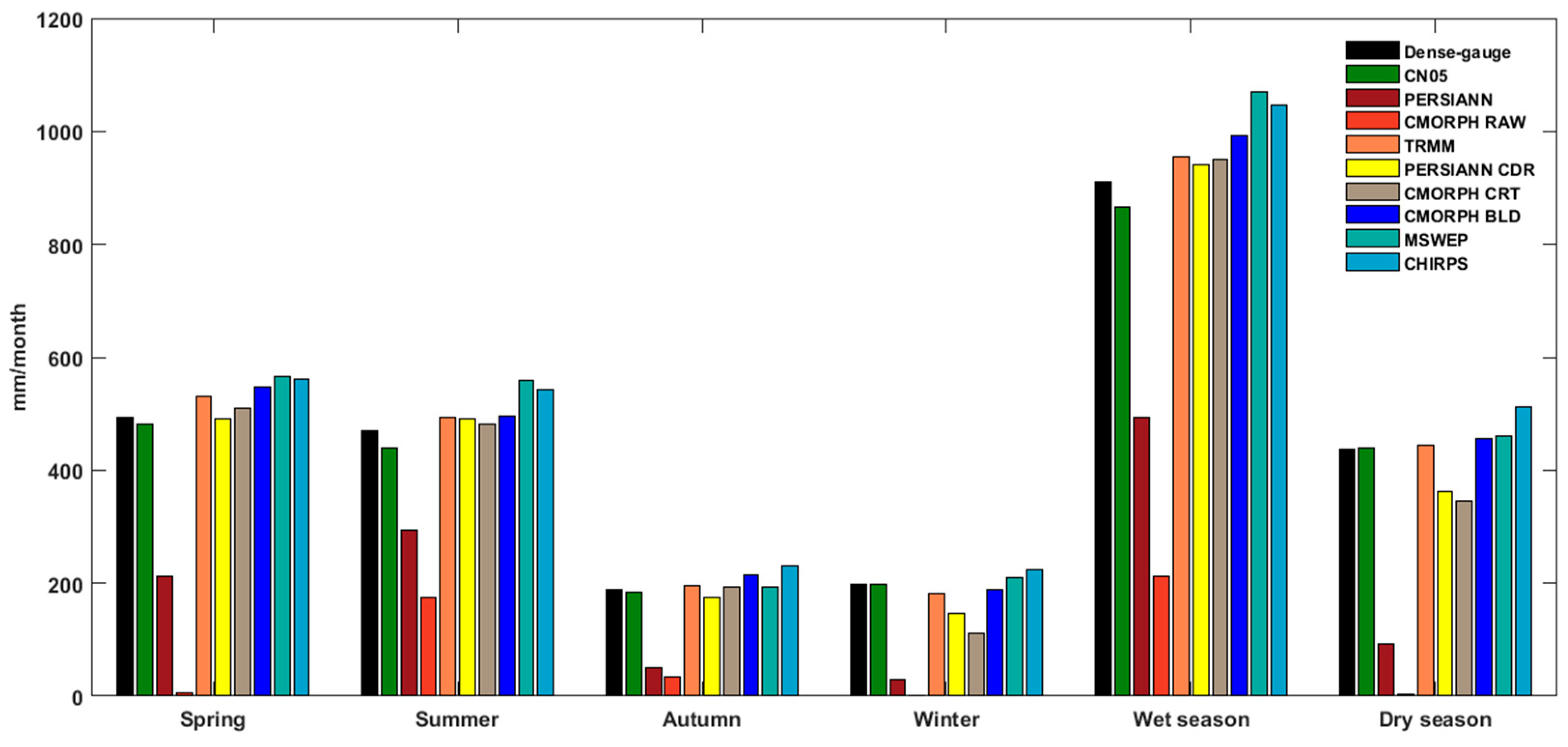
Figure 2 presents the seasonality (spring: March–May, summer: June–August, autumn: September–November, winter: December–February; wet season: April–September and dry season: October–March) of the mean precipitation for all ten precipitation datasets (eight satellite-based precipitation datasets, one gauged precipitation (i.e., the dense-gauge dataset), and one gauge-interpolated precipitation (i.e., CN05)). All stations or grids within the watershed are averaged to a single time series to calculate the seasonal mean values. The figure graphically demonstrates that CN05 agrees well with the dense-gauge observation for all four seasons. Specifically, CN05 presents a small RB within ±7.0% for seasonal precipitation (−2.4% for spring, −6.1% for summer, −1.7% for autumn, and 0.3% for winter). With the exception of satellite-only datasets, which considerably underestimate the precipitation for all seasons, the satellite-based datasets also reasonably represent the observed seasonality. However, all of them are worse than CN05 for all seasons. The better performance of PERSIANN CDR among satellite-based datasets for seasonal precipitation, especially in spring, summer, and autumn, could reflect the effects of its blending strategies. PERSIANN CDR maintains monthly precipitation that is consistent with the monthly GPCP, and GPCP is mainly composed of gauged precipitation datasets (e.g., GPCC) [70]. In addition, all the satellite-gauge datasets overestimate the dense-gauge precipitation in summer and the wet season while underestimating in winter. In addition, both blended datasets (MSWEP and CHIRPS) overestimate the precipitation all year round. TRMM, CMORPH BLD, and MSWEP fit the dense-gauge precipitation better in the dry season than the wet season, while PERSIANN CDR, CMORPH CRT, CHIRPS, and satellite-only datasets perform better in the wet season than the dry season.
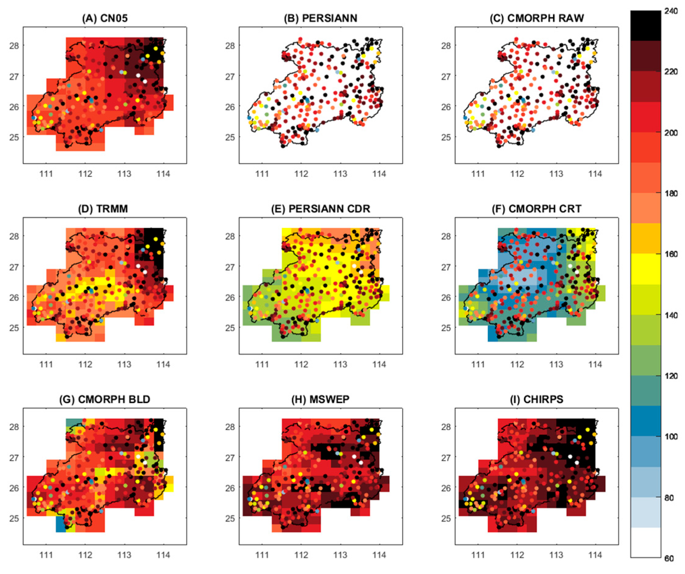
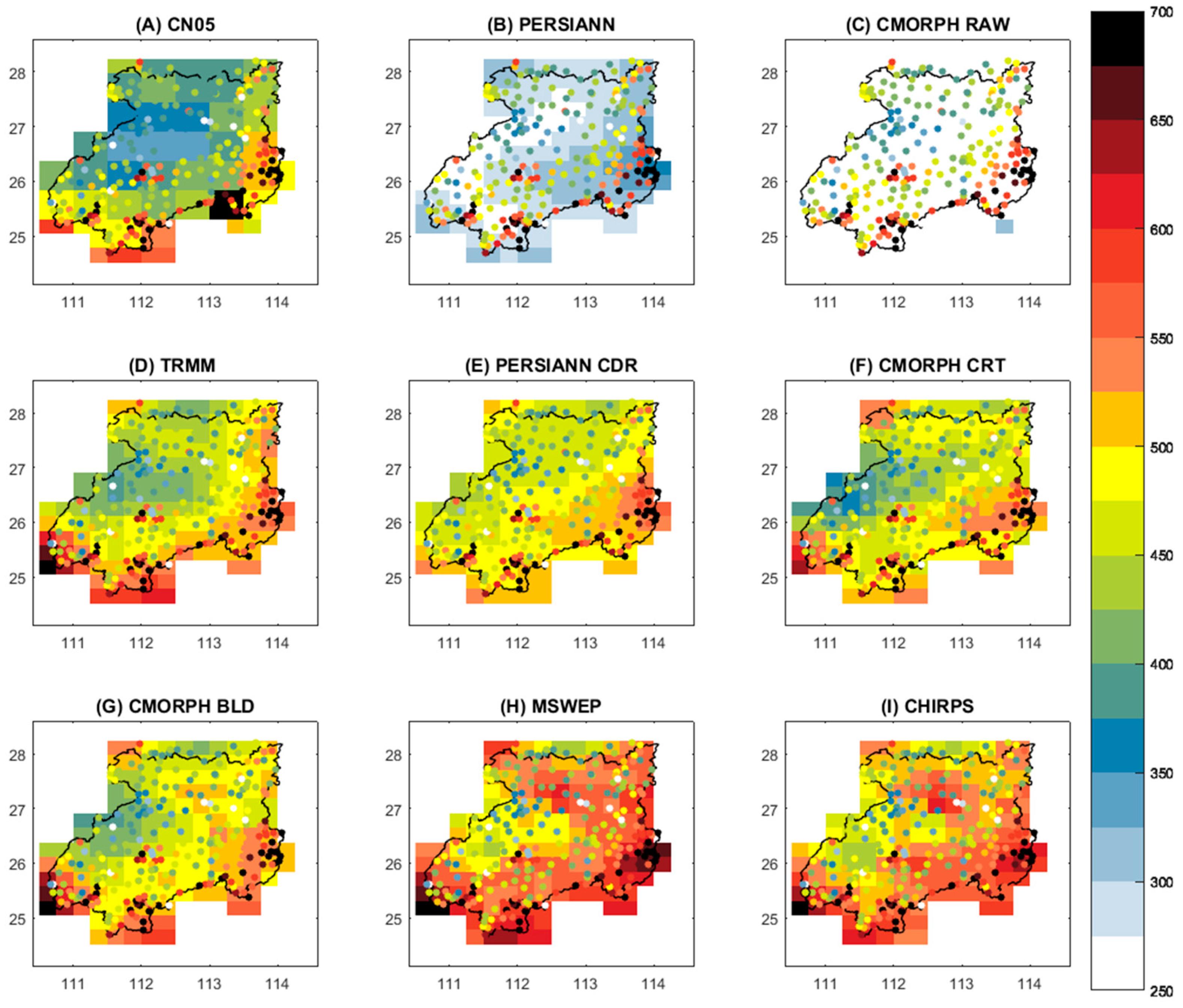
The spatial distributions of summer precipitation are also presented for all datasets in Figure 3. The dense-gauge datasets are presented as color dots, while all the other datasets are presented as grids. Generally, summer precipitation is heavier in high elevation areas (southeastern, southwestern, and southern parts) than in other regions. CN05 clearly missed quite some regional intensive precipitation (such as the heavy precipitation in the southeastern parts of the region), which can even be captured by MSWEP and CHIRPS. The bad performance of CN05 may be caused by two reasons: (1) its lower spatial resolution (0.5° × 0.5°) and (2) its less gauged source data compared with the dense-gauged dataset. Satellite-only datasets underestimate precipitation for all grids, even though PERSIANN can capture the heavy precipitation signal in mountain areas. Although all satellite-gauge datasets could capture this spatial distribution pattern, these datasets still underestimate the heavy precipitation in mountain areas (southern and southeastern parts) while overestimating the small precipitation in central plain regions. The spatial distributions of winter precipitation, as shown in Appendix B in Figure A1, display similar patterns, as CN05 still performs relatively worse than the two blended datasets: MSWEP and CHIRPS. The better performance of blended datasets for the spatial distribution of seasonal precipitation may be due to their reanalysis components.

4.1.2. Error Structures of Precipitation Datasets

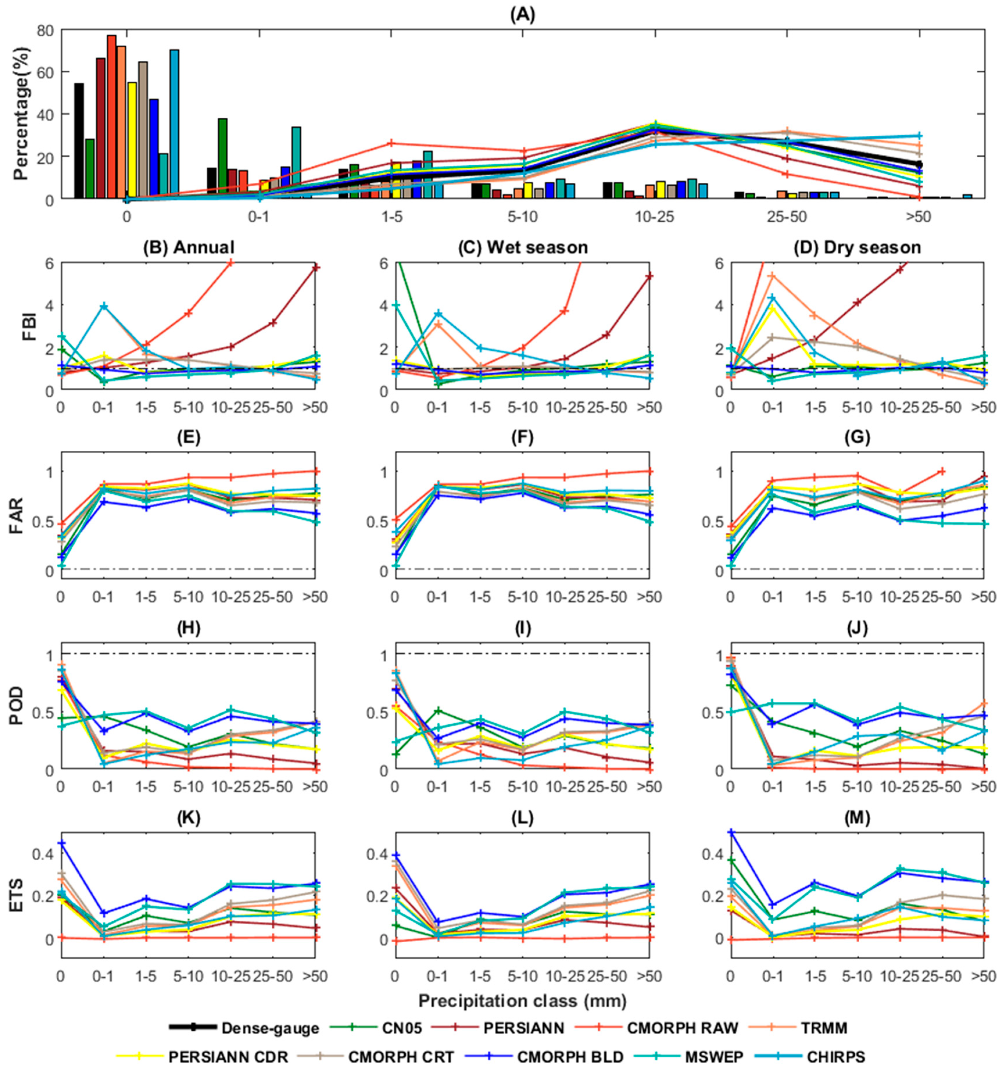
Figure 4A presents two types of the daily gridded precipitation information for the dense-gauge, CN05, and eight satellite-based datasets: (1) bar charts represent the frequency distribution of precipitation under seven different rain rate classes (0, 0–1, 1–5, 5–10, 10–25, 25–50 and >50 mm/day) and (2) line charts represent the contribution of the precipitation amount under each rain rate class to the total precipitation. As shown in the bar charts, PERSIANN CDR, CMORPH CRT, and CMORPH BLD are close to the gauged counterparts of where the precipitation frequencies decrease from 0 to 0–1 mm and slightly increase under the 1–5 mm class, and then decrease until the >50 mm class. These tendencies of precipitation frequency under the 0, 0–1, and 1–5 mm classes are inaccurately represented by MSWEP. Another two satellite-based datasets (TRMM and CHIRPS) overestimate the frequencies of no rain (0 mm) and heavy rain (>50 mm) and underestimate little rain (0–1 mm). Line charts show that the largest precipitation contribution of all datasets except for TRMM and CMORPH CRT occurs at the 10–25 mm class. Large differences in the precipitation contribution among datasets occur at the 25–50 mm and >50 mm classes.
The detection errors of each satellite-based dataset are quantified based on the FBI, FAR, POD, and ETS in terms of the 11-year (2003–2013) annual, wet season, and dry season precipitation processes. Figure 4B presents the distribution of the FBI for nine precipitation datasets (CN05 and eight satellite-based datasets). FBI values of CMORPH RAW at the 25–50 (13.66) and >50 (89.35) intervals being larger than 6 are not demonstrated, which is the same as Figure 4C,D. Although both satellite-gauge and blended datasets poorly simulate the annual FBI values in the rain rates of 0 mm (e.g., the FBI of MSWEP is 2.55) and 0–1 mm (e.g., the FBI of TRMM is 3.95), they overall outperform the satellite-only categories, which have worse annual FBI results under more than half of the rain rate classes (Figure 4B). Figure 4C,D further demonstrates that more overestimations of FBI values of satellite-only datasets under most rain rate classes (5–10, 10–25, 25–50, and >50 mm) occur in the dry season than the wet season. The larger underestimation of precipitation events in the dry season is in good agreement with the seasonal precipitation amount in Section 4.1.1 and could further explain the sources of poor performances for satellite-only datasets. This may be because of the underestimation of precipitation events with the rain rate classes being larger than 10 mm during the wet season and the underestimation of all precipitation events during the dry season. As the rain rate class increases, the FBI of satellite-gauge datasets improves until the precipitation class exceeds 50 mm for both seasons. The annual FBI values of CMORPH CRT (0.78), TRMM (0.62), and CHIRPS (0.49) at this class are less than 1, indicating that these datasets overestimate the number of heavy rain events. This may also explain the overestimation of the percentage of heavy rains (Figure 4A).
FAR, POD, and ETS of satellite-based datasets also show obvious seasonal patterns. Two satellite-only datasets significantly deteriorate with the increasing rain rate classes in terms of the annual FBI, FAR, and POD, indicating their inability to capture the heavy precipitation. These two datasets clearly perform better in the wet season than in the dry season, especially in terms of the POD (Figure 4I,J) and ETS (Figure 4L,M). However, CMORPH BLD and MSWEP show an opposite seasonal pattern, as the better performance occurs in the dry season than the wet season in terms of the three statistics. In addition, both of them maintain their superiority among all the satellite-gauge datasets. Although gauge-interpolated CN05 shows relatively worse performances than CMORPH BLD and MSWEP, it shares similar seasonal patterns with them and also outperforms the other six satellite-based datasets with regard to POD and ETS under the most rain rate classes (0–1, 1–5, 5–10, and 10–25 mm).
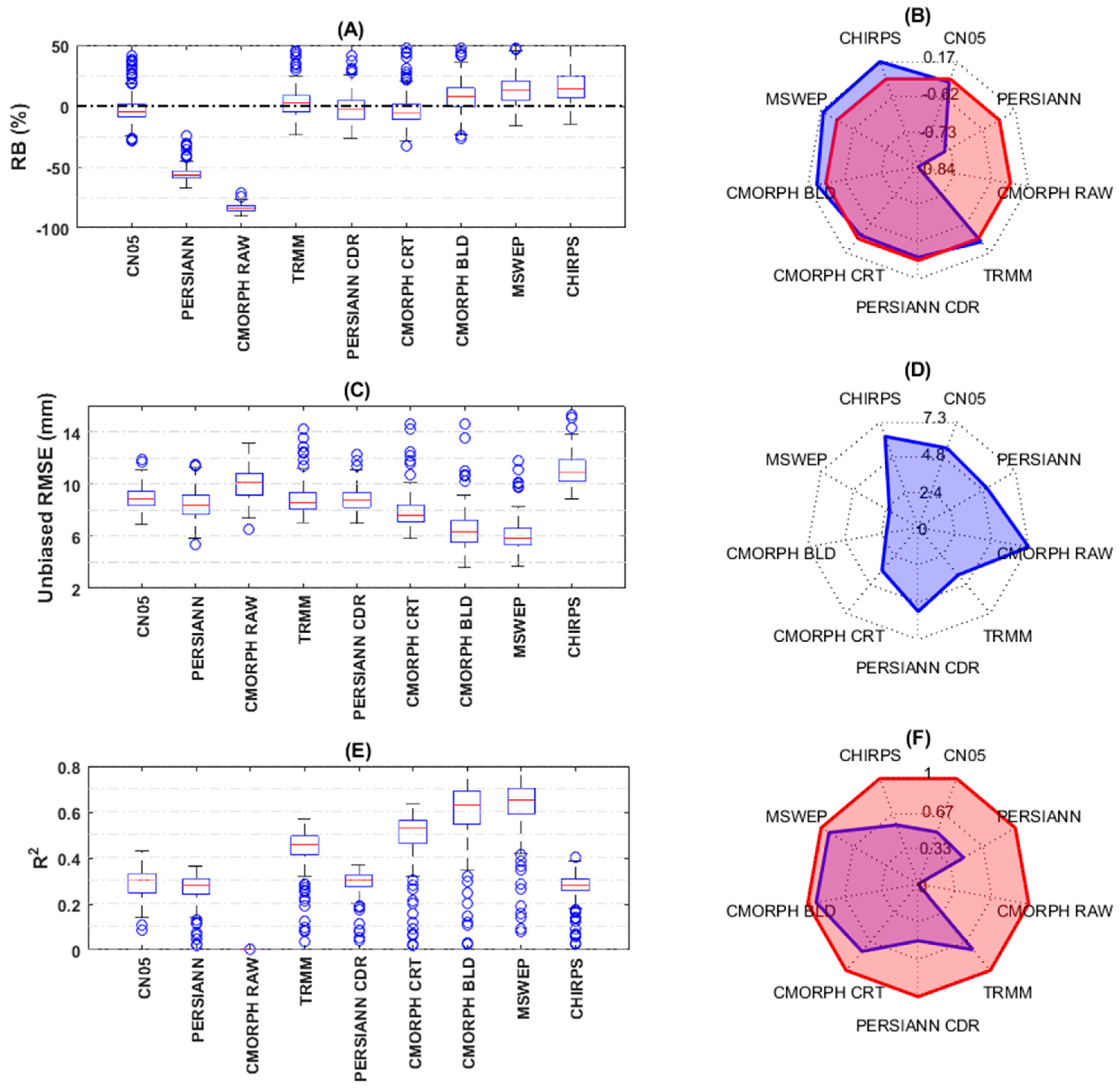
Figure 5 shows the RB, ubRMSE, and R 2 of nine precipitation datasets (CN05 and eight satellite-based datasets) at both grid (shown as boxplots) and watershed-average scales (shown as radar plots). Generally, the performances of each precipitation dataset under two different scales are basically consistent in terms of all three quantitative statistics. Figure 5A,B show that CN05 presents a better RB than the eight satellite-based datasets. Among all satellite-gauge datasets, TRMM, PERSIANN CDR, and CMORPH CRT show the smallest RBs, indicating their smaller systematic errors, at both grid and watershed-averaged scales. CMORPH BLD and two blended datasets (MSWEP and CHIRPS) generally show positive RB under both scales, especially for CHIRPS, which overestimates the daily precipitation for more than 86.1% of the grids and has an RB of 16.5% at the watershed-average scale. In contrast, satellite-only datasets considerably underestimate the mean precipitation at both scales.
Random errors of CN05 and satellite-based datasets are quantified using the ubRMSE (Figure 5C). CN05 shows relatively larger random errors than the satellite-based datasets except for CMORPH RAW and CHIRPS. In addition, large differences are observed among satellite-based datasets. Specifically, CMORPH BLD presents the smallest ubRMSE with the median value of 6.31 mm at the grid scale (Figure 5C) and 2.09 mm at the watershed-average scale (Figure 5D), while CHIRPS presents the largest ubRMSE with the median value of 10.94 mm at the grid scale and 6.28 mm at the watershed-average scale. MSWEP performs the best among all nine precipitation datasets with a median value of 5.83 mm at the grid scale and 2.14 mm at the watershed-average scale.
Figure 5E,F presents the R 2 values for all nine precipitation datasets, and both clearly reflect the influence of the blending methods and the incorporated gauged datasets on R 2 . Datasets designed to provide the best instantaneous accuracy of precipitation (TRMM, CMORPH CRT, CMORPH BLD, and MSWEP) perform relatively better than those aimed to achieve the most temporally homogeneous record (PERSIANN CDR and CHIRPS). Within the four better-behaved satellite-based datasets, those that directly incorporate daily gauge data (CMORPH BLD and MSWEP) clearly perform better than those that directly incorporated monthly gauge data (TRMM and CMORPH CRT). Two satellite-only datasets show the worst performance among all the satellite-based datasets. Similarly, CN05 is also less correlated with the dense-gauge dataset than half of the satellite-based datasets (TRMM, CMORPH CRT, CMORPH BLD, and MSWEP).

4.1.3. Simulation of Extreme Precipitation

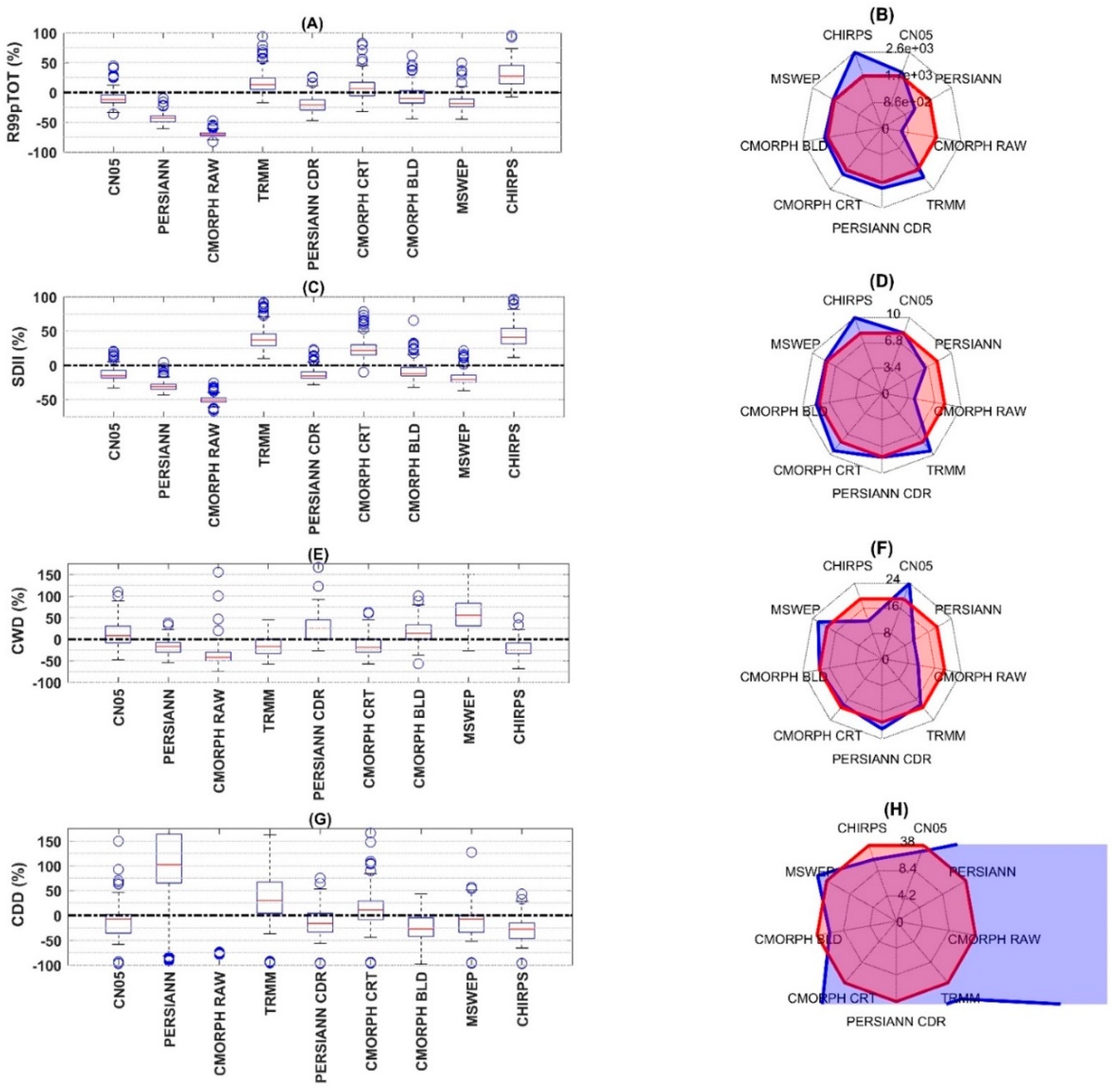
The results of four extreme precipitation statistics are presented in Figure 6 for nine datasets (CN05 and eight satellite-based datasets) at both grid (shown as relative bias compared to the dense-gauge precipitation dataset in boxplots) and watershed (shown as the absolute value in radar plots) scales. In the radar plots, red and blue lines represent the results of the dense-gauge and each dataset, respectively.
R99pTOT (Figure 6A,B) reflects the total precipitation of heavy rain. The R99pTOT values of satellite-gauge and blended datasets except PERSIANN CDR and CHIRPS are similar to the dense-gauge observation, especially for more than 50% grids having biases within ±20.0% at the grid scale. Specifically, PERSIANN CDR underestimates R99pTOT with more than 56.3% of grids having negative bias being smaller than −20% and a relative bias of 9.3% at the watershed scale. However, CHIRPS overestimates R99pTOT at both scales (with more than 63.6% of grids having positive bias being larger than 20%, and a relative bias of 45.3% at the watershed scale). Additionally, two satellite-only datasets underestimate R99TOT.
The SDII values are shown in Figure 6C,D, and the similar results of SDII and R99pTOT can be explained by two factors: (1) heavy precipitation accounts for a large proportion of the annual precipitation amount, and (2) the number of wet days is similar for all nine datasets. The CWD is presented in Figure 6E,F at the grid and watershed-average scales, respectively. The CDD is presented in Figure 6G,H. The results show that CMORPH BLD maintains its superiority among all the datasets in simulating these two extreme statistics. However, the other seven satellite-based datasets could not accurately capture the CDD and the CWD at the same time, especially for the CDD, which is used as a criterion for representing droughts. For example, CMORPH CRT shows a small bias of CWD at both grid (with more than half of the grids have a bias of between ±10.0%) and watershed-average scales (CMORPH CRT: 18 days and the dense-gauge: 19 days). On the contrary, the CDD of CMORPH CRT is not accurately estimated with more than 50.0% of the grids having a bias larger than 10.0% and bias of 44.7% at the watershed-average scale (CMORPH CRT: 55 days and the dense-gauge: 38 days).
CN05 better represents these four extreme precipitation statistics than all satellite-based datasets, especially for CDD, as shown in Figure 6G,H. It also shows tiny detection and systematic errors in the previous comparison in Section 4.1.2. However, CN05 misses quite some regional intensive seasonal precipitation and has larger random errors and worse R 2 compared with more than half of the satellite-based datasets. In other words, the bad performance of CN05 indicates that some satellite-based datasets are effective in representing the spatial distribution of precipitation. However, this effect can be missed by gauge-interpolated datasets using sparse gauges with a relatively coarser spatial resolution. Therefore, there is a risk of having CN05 as the reference when investigating the statistical properties of satellite-based precipitation, especially for high-precision datasets.

4.2. Hydrological Simulations

Eight satellite-based datasets and gauge-interpolated CN05 are further compared against the dense-gauge dataset in hydrological modeling by both XAJ and SWAT models calibrated by observed streamflow. Both models are adequately calibrated with NSE values of 0.89 (XAJ) and 0.86 (SWAT) for calibration, and 0.89 (XAJ) and 0.84 (SWAT) for validation (Table 3).
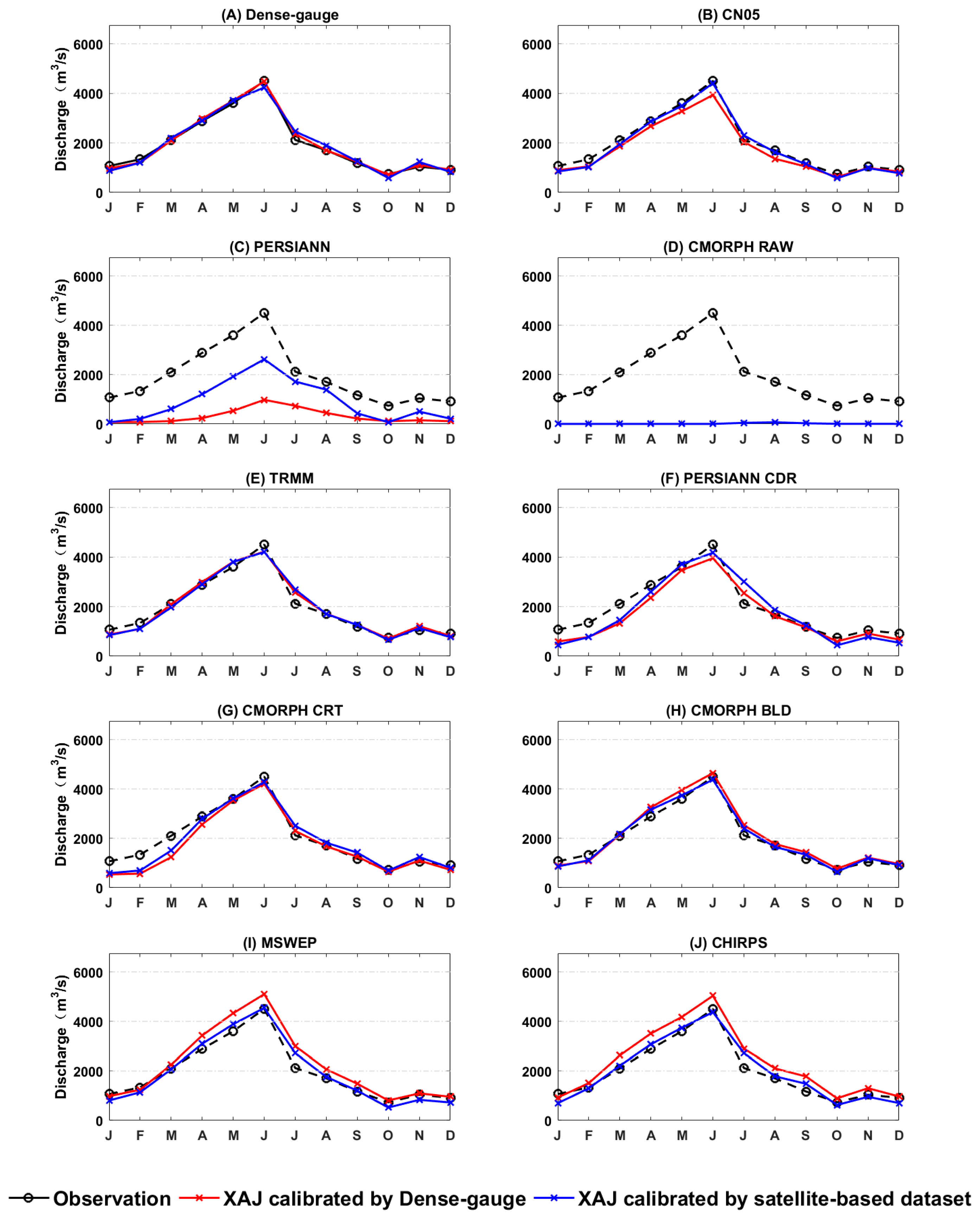
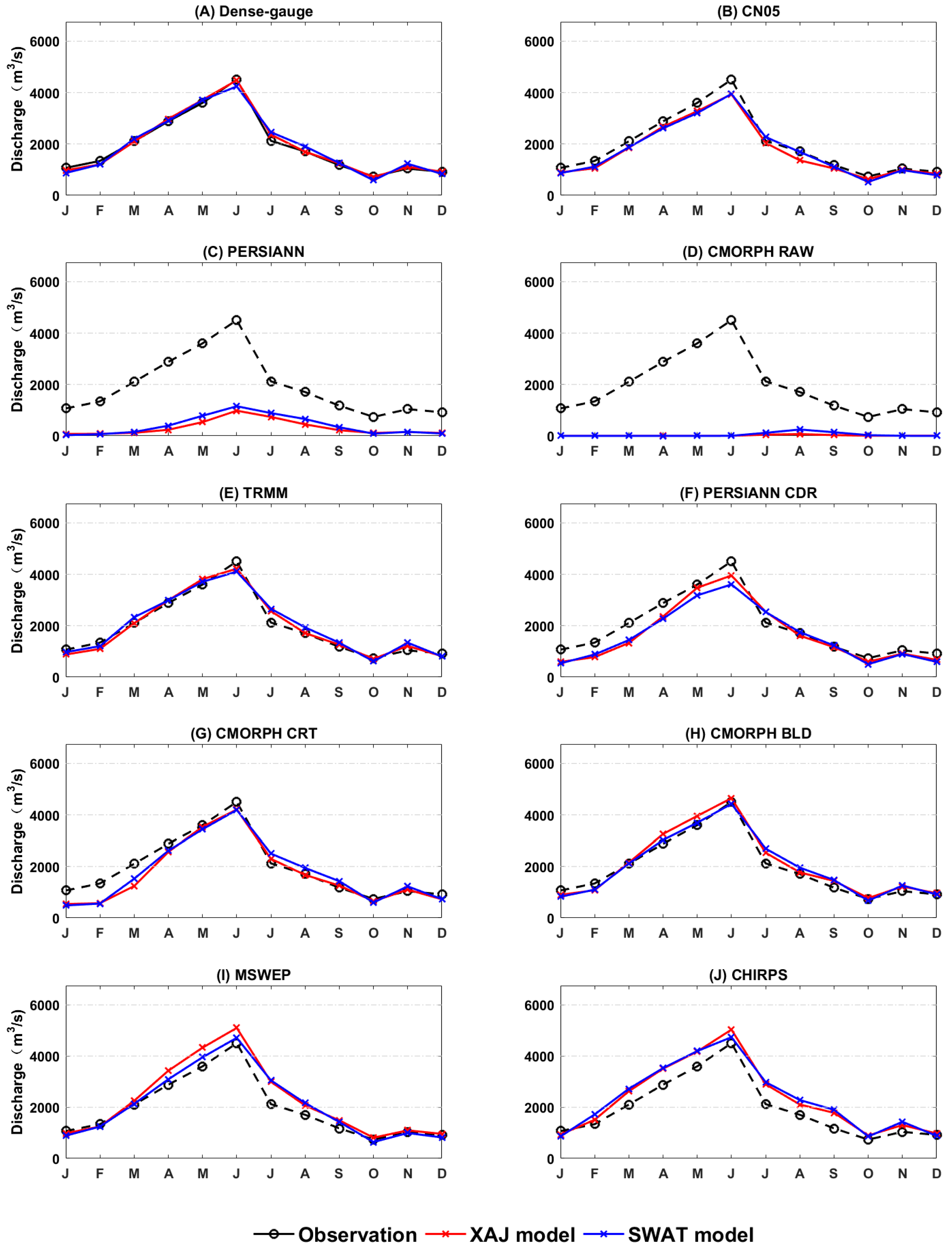
For illustrating the intra-annual variability of the hydrological process, Figure 7 shows the mean monthly hydrographs of observed and the simulated streamflow of the dense-gauge and the other nine precipitation datasets based on two models. The reason for using a monthly hydrograph rather than a daily hydrograph is to avoid noises when calculating the climatology due to the relatively short time period (i.e., 10 years) [95,96]. It can be observed that (1) the most precise simulation of discharge is achieved by the gauge-interpolated CN05 among all nine precipitation datasets. CMORPH BLD, MSWEP, TRMM, and CMORPH CRT offer better performance than the other satellite-based datasets. CHIRPS and PERSIANN CDR, respectively, overestimate and underestimate the observed discharge for almost the whole year. (2) During the flood periods (from April to August), the simulation processes of both the dense-gauge and the other nine datasets based on the XAJ model are obviously larger than results based on the SWAT model. Similar results were also discovered by Xu et al. [3], who used XAJ and SWAT models to test the ability of two reanalysis datasets in simulating flood events in the Xiangjiang River Basin.
To further quantify the performance of satellite-based datasets in representing streamflow time series, the NSE values of two hydrological models based on daily streamflow are calculated and presented in Table 3. Results based on the XAJ model show that three satellite-gauge precipitation datasets (TRMM, CMORPH CRT, and CMORPH BLD) and blended datasets (MSWEP) are satisfactory in simulating streamflow time series, with NSE being larger than 0.72. CMORPH BLD (NSE = 0.84) outperforms all other satellite-based datasets. CHIRPS (NSE = 0.44) and PERSIANN CDR (NSE = 0.56) show moderate performances. Satellite-only datasets cannot represent the observed streamflow time series with NSE = −0.97 for CMORPH RAW and NSE = −0.40 for PERSIANN. The semi-distributed SWAT shows the similar daily simulation performance of each dataset with the lumped XAJ, but the performance of satellite-gauge datasets in SWAT is slightly worse than that in the XAJ except for PERSIANN CDR. Similar to PERSIANN CDR, both blended datasets, CHIRPS (NSE = 0.44/0.48 for XAJ/SWAT) and MSWEP (NSE = 0.78/0.79 for XAJ/SWAT), perform better in SWAT than in XAJ. Despite some differences in the simulation performances of the two models, the relative sort orders of the datasets based on NSE are almost consistent in both models. The best simulation was achieved by satellite-gauge CMORPH BLD, which was followed by blended MSWEP, TRMM, and CMORPH CRT. CHIRPS. PERSIANN CDR performed moderately; however, satellite-only datasets showed the worst performance. This consistency indicates that using different models does not significantly alter the relative performances of streamflow simulation of satellite-based precipitation datasets.
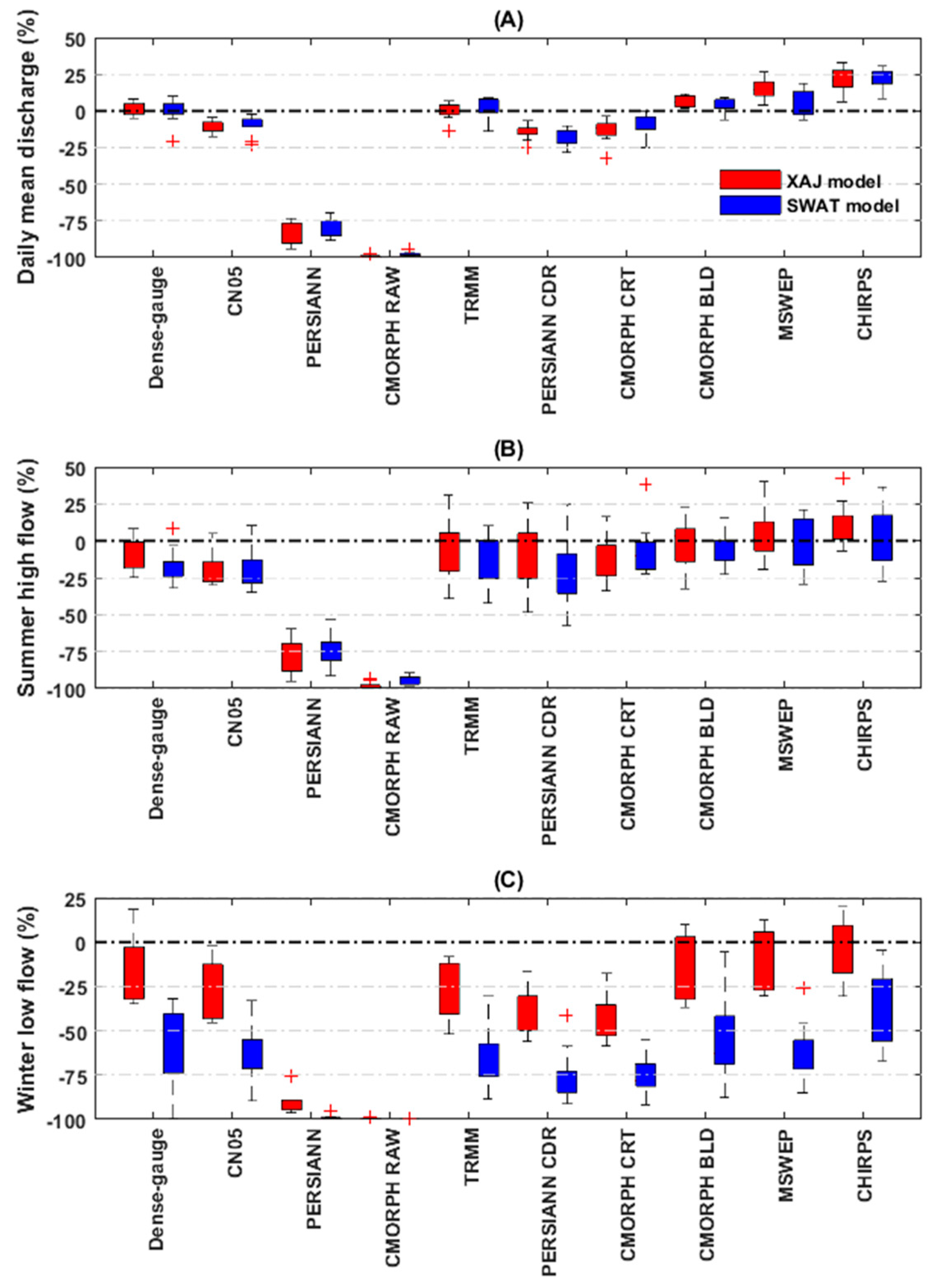
Three hydrological statistics (daily mean discharge, winter low flow, and summer high flow) are further used to compare the daily simulated discharge of both the dense-gauge and the nine alternative datasets against their observed counterparts. Figure 8 presents the annualized results (shown as the relative bias between the simulated discharge of each precipitation dataset and the observed discharge) of three statistics from 2004 to 2013. XAJ and SWAT models show similar results for daily mean discharge (Figure 8A); however, SWAT obviously underestimates the other two hydrological statistics (Figure 8B,C), especially for the winter low flow. Based on three statistics, CMORPH BLD consistently performs better than other satellite-gauge datasets. PERSIANN CDR and CHIRPS respectively underestimate and overestimate the observed discharge for both models. Blended MSWEP performs well, although its daily maxima discharge in the XAJ model shows an obvious overestimation (the results of 8 years are more than 0) and underestimation in the SWAT model (the results of 7 years are less than 0). Similar to previously used indexes, satellite-only datasets still show the worst performance.

4.3. Error Propagation

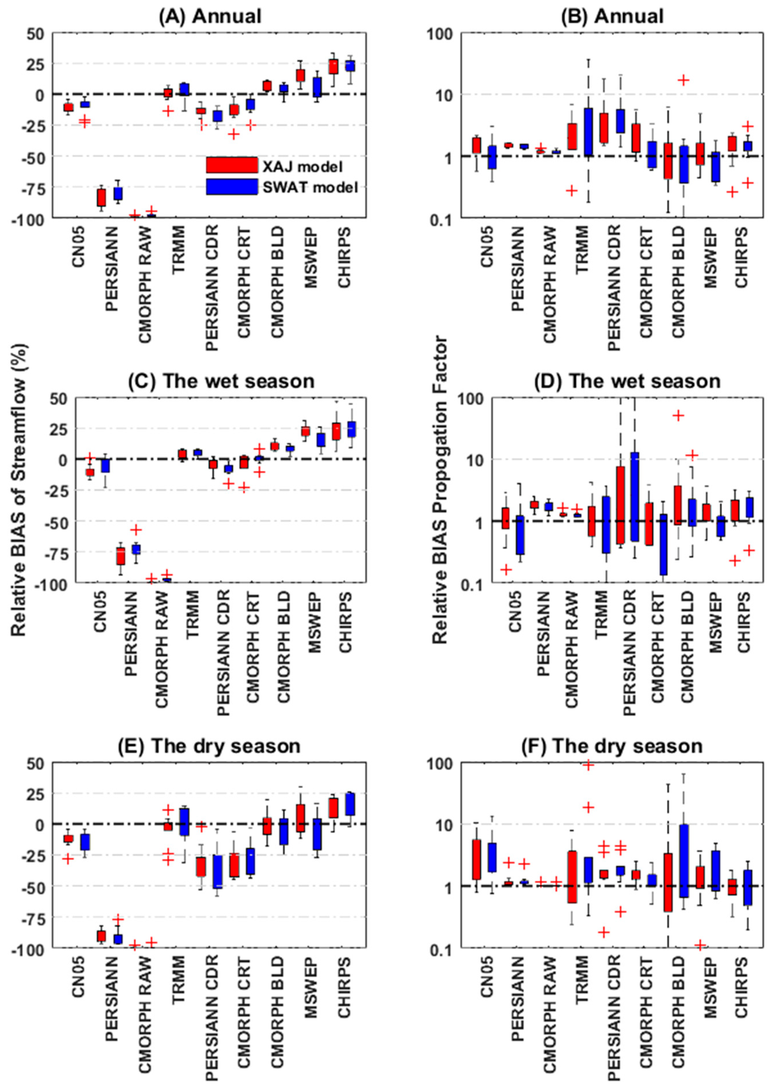
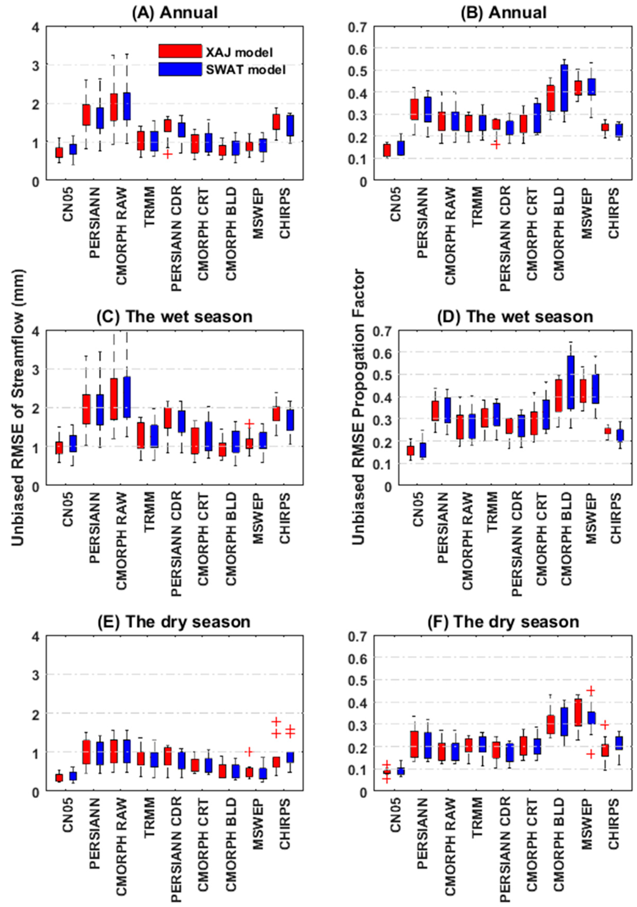
RB and ubRMSE of streamflow respectively reflect the systematic and random errors of each dataset in simulating the streamflow. Figure 9 and Figure 10 respectively show the RB and ubRMSE of annual, wet, and dry seasons streamflow and their corresponding propagation factors ( γ R B and   γ u b R M S E ) simulated using CN05 and eight satellite-based precipitation datasets from 2004 to 2013.

4.3.1. Systematic Error Propagation

Generally, TRMM, with the minimal RB (systematic error) of annual streamflow performs the best among all datasets, which is then followed by CMORPH CRT and CMORPH BLD, displaying comparable performance with CN05 (Figure 9A). Two satellite-only datasets considerably underestimate the annual streamflow. However, their results of the systematic error propagation factor ( γ R B shown in Figure 9B) are larger than 1, indicating amplification of the systematic error when translating the precipitation into a runoff. TRMM, PERSIANN CDR, and CHIRPS have the same amplified effect for the systematic error of the precipitation, while γ R B values for the other five datasets are around 1.
There is a seasonal trend for the RB of streamflow for all datasets in which the range of RB values for the wet season streamflow (Figure 9C) is much smaller than that for the dry season (Figure 9E). This narrow RB range means a smaller inter-annual difference in the wet season. As for RB, six out of nine datasets (all datasets except CMORPH BLD, MSWEP, and CHIRPS) show smaller RBs (closer to 0) in the wet season than in the dry season. Thus, the more apparent amplification of the systematic error of precipitation to runoff (the larger results of γ R B ) occurs in the dry season compared to the wet season for nearly all nine datasets except for satellite-only datasets (Figure 9D,F).
Moreover, the hydrological models also influence the RB of streamflow. During the wet season, SWAT generally performs much better than XAJ for more than half of the datasets (all datasets except for TRMM, PERSIANN, and CHIRPS, Figure 9C). While during the dry season, XAJ outperforms SWAT for more than half of the datasets (all datasets except for CMORPH CRT and MSWEP, Figure 9E).

4.3.2. Random Error Propagation

Figure 10A demonstrates that the streamflow values of ubRMSE are not distinctive among nine datasets, except for two satellite-only data, which have significantly larger values. Among the rest of the datasets, PERSIANN CDR and CHIRPS show the largest random errors of streamflow. CN05 shows the minimum ubRMSE of streamflow; however, this is different from its relatively larger ubRMSE of the precipitation (as demonstrated in Section 4.1.2). This discrepancy in the ubRMSE of precipitation and streamflow for CN05 is due to its largest dampening effect of random error. All the other eight datasets have similar dampening effects with γ u b R M S E being smaller than 1 (Figure 10B), and CMORPH BLD along with MSWEP have the largest γ u b R M S E among these datasets.
ubRMSE of streamflow also has a seasonal trend with its values and ranges in the wet season (Figure 10C) being larger than those in the dry season (Figure 10E) for all datasets. This seasonal difference also applies to the random error propagation factor γ u b R M S E (Figure 10D,F). ubRMSE of the same precipitation dataset generated from different hydrological models is different (Figure 10C,E). Specifically, SWAT generates a larger ubRMSE than that of the XAJ model for nearly all datasets (nine datasets except for PERSIANN CDR and CHIRPS), especially during the wet season (Figure 10D,F).
Satellite-only datasets directly estimate precipitation through PMW or IR sensors [22,23,24]. Their worst performances among all eight satellite-based datasets reflect the defectiveness of the existent remote sensing retrievals algorithms and the necessity to blend with gauged measurement to account for their limited abilities, such as distinguishing rain particles and electromagnetic interferences from rough terrain and trees to sensors [26]. Theoretically, PMW is more accurate than VIS–IR, because the former physically links the sensors’ signal to the size and phase of the hydrometeors, which is presented within the observed atmospheric column [1,24,91]. However, CMORPH RAW (mainly based primarily on PMW) performs worse than PERSIANN (mainly based on IR), which is opposite for some other regional studies in the Asian monsoon regions, such as Japan [97] and the Tibet Plateau [98]. This inconsistent result may reflect the influence of integrating methods (PMW and IR) on the performance of satellite-only datasets and the region-dependent nature of these methods.
Compared with satellite-only datasets (CMORPH RAW and PERSIANN), better performances in both precipitation and hydrological simulations are clearly achieved by their improved satellite-gauge versions (CMORPH CRT, CMORPH BLD, and PERSIANN CDR). This improvement proves the validity of the blending algorithms using gauge precipitation to enhance the precipitation estimation performances of the satellite-only datasets. Satellite-gauge CMORPH BLD outperforms all satellite-gauge datasets in both precipitation and hydrological simulations, which is mainly due to the effectiveness of using bias correction and blending algorithms by incorporating the daily precipitation gauge dataset to improve CMORPH RAW [36]. Among blended datasets, MSWEP shows comparable good performance with CMORPH BLD. The superiority of MSWEP could be mainly explained by two factors: (1) the gauged component utilized by MSWEP takes up a higher proportion (30.0% to 50.0%) in the final precipitation dataset compared to the other satellite-based datasets; and (2) the reanalysis data used in MSWEP may bring more potential information [71,99].
CN05 outperforms all satellite-based datasets in hydrological simulation. This satisfactory performance suggests that CN05 is fully able to act as the proxy of the dense-gauge precipitation dataset in the hydrological simulation in the Xiangjiang River Basin, although it could not act as the reference data to directly evaluate the statistical properties of satellite-based precipitation.
Additionally, the datasets used for model calibration would influence the hydrological performances of satellite-based datasets for the validation period, and many studies suggested recalibrating hydrological models directly using satellite-based datasets [60,100,101]. However, only the dense-gauge precipitation was used in this study to calibrate the hydrological models, and all satellite-based datasets then used the same set of optimal parameters for hydrological modeling. This is based on the assumption that the dense-gauge dataset is more accurate than the satellite-based datasets, excluding the effects of uncertainty in model parameters on hydrological simulations. Even though the satellite product-forced model performance may be degraded, when using the dense-gauge precipitation for model calibration, all satellite-based datasets used the same set of optimal parameters for hydrological modeling. In addition, one test based on the XAJ model has been conducted to prove that the calibration dataset would not change the relative hydrological performance of these satellite-based datasets, which are shown in Appendix C as Table A1 (NSE value for both calibration and validation periods) and Figure A1 (mean monthly hydrograph during 2004–2013). Therefore, it is rational to compare the performance of each satellite-based dataset. For those watersheds where the dense-gauge precipitation dataset is not available, the hydrological model may be calibrated using satellite-based datasets or other gridded datasets.

5. Conclusions

This study evaluates eight high-resolution satellite-based precipitation datasets (satellite-only: PERSIANN and CMORPH RAW, satellite-gauge: TRMM PERSIANN CDR, CMORPH CRT and CMORPH BLD and blended: MSWEP and CHIRPS) and a gauge-interpolated CN05 based on a dense-gauge dataset for hydrological modeling over a monsoon prone watershed in China. We can draw the following conclusions:
(1)
All satellite-gauge and blended datasets are able to capture the seasonality of precipitation in the study region, even though biases are observed. Specifically, the satellite-gauge CMORPH BLD generally outperforms all other satellite-based datasets with the smallest detection, systematic, random errors, and most precise extreme precipitation simulation. However, satellite-only datasets perform the worst with respect to almost all the precipitation indices. Although CN05 presents the smallest systematic errors, CN05 cannot be used as the reference data to statistical analysis of the satellite-based datasets because it is missing some seasonal local precipitation and has larger random errors and a smaller R 2 .
(2)
There are large differences among satellite-gauge datasets in hydrological simulations. Datasets designed to provide the best instantaneous precipitation (TRMM, CMORPH CRT, CMORPH BLD, and MSWEP) perform better than those designed to achieve the most temporally homogeneous record (PERSIANN CDR and CHIRPS). Among the four better-behaved datasets, two directly incorporating daily gauge data (CMORPH BLD and MSWEP) outperform two directly incorporating monthly gauge data (TRMM and CMORPH CRT). However, satellite-only datasets (CMORPH RAW and PERSIANN) are the least capable of simulating streamflow, which is not recommended to use in the hydrological application. CN05 outperforms all satellite-based datasets in the hydrological simulation, indicating its capability to act as reference data during the hydrological evaluation.
(3)
With different model structures, XAJ and SWAT models perform differently for each satellite-based dataset, and differences in model performances also depend on seasons. Generally, the XAJ model performs better than the SWAT model in terms of random errors of streamflow simulations for both wet and dry seasons and in terms of systematic errors for the dry season. However, compared with the hydrological model uncertainties, the uncertainties from different satellite-based datasets dominate the uncertainty of hydrological simulation. In other words, the hydrological model structure does not affect the overall performance ranking of satellite-based precipitation datasets in hydrological simulations in this study.
(4)
The random error from all datasets show a general decrease from precipitation to runoff with γ u b R M S E being smaller than 1, but this does not hold for the systematic error with γ R B varying in different datasets. In addition, the seasons and the hydrological models affect the error propagation from precipitation to streamflow for all datasets. The systematic ( γ R B ) and random ( γ u b R M S E ) error propagation factors of the wet season are larger than those of the dry season. The XAJ model shows a more amplified error propagation effect of the systematic errors, while the random errors are more amplified by the SWAT model.
There are still some limitations in this study. For example, the eight satellite-based datasets were compared over only one monsoon-prone watershed, and the conclusion may not be the same for other regions. In addition, the differences between using a dense-gauge dataset and satellite-based datasets to calibrate hydrological models were not fully investigated. For some data-lacking regions, the satellite-based datasets may be directly used to calibrate the hydrological models when the dense-gauge dataset is available. Therefore, in future studies, more watersheds from various climate regimes should be used to generalize the conclusions drawn from this study. In addition, the impacts of using different satellite-based datasets to calibrate the hydrological models on hydrological performances also need to be investigated.

Author Contributions

Conceptualization, J.C. and Z.L.; Data curation, Z.L., J.W. and W.Q.; Formal analysis, Z.L., L.L., J.W. and W.Q.; Funding acquisition, J.C.; Investigation, J.C., Z.L., L.L., J.W. and W.Q.; Methodology, J.C., Z.L., L.L., C.-Y.X. and J.-S.K.; Project administration, J.C.; Resources, C.-Y.X.; Supervision, J.C., C.-Y.X. and J.-S.K.; Validation, Z.L.; Visualization, J.C. and Z.L.; Writing—original draft, J.C. and Z.L.; Writing—review and editing, J.C. and Z.L. All authors have read and agreed to the published version of the manuscript.

Funding

This work was partially supported by the National Natural Science Foundation of China (Grant No. 52079093, 51779176), the Hubei Provincial Natural Science Foundation of China (Grant No. 2020CFA100), and the Overseas Expertise Introduction Project for Discipline Innovation (111 Project) (Grant No. B18037).

Acknowledgments

The authors would like to acknowledge the Water Resources Bureau of Hunan Province for providing gauged precipitation data and the China Meteorological Data Sharing System for providing temperature data and gridded datasets. The authors also thank all of the organizations for providing the satellite-based datasets, namely, the Goddard Earth Sciences Data and Information Services Center (TRMM), NOAA Climate Prediction Center (CMORPH RAW, CMORPH CRT, and CMORPH BLD), NOAA National Climatic Data Center (PERSIANN and PERSIANN CDR), Climate Hazards Group (CHIRPS) and Hylke Beck from Princeton University, the developer of MSWEP.

Conflicts of Interest

The authors declare no conflict of interest.

Appendix A

A detailed description of the satellite-based precipitation datasets used in this study.

Appendix A.1. Tropical Rainfall Measuring Mission 3B42 Dataset (TRMM)

TRMM 3B42, one of the TRMM Multi-satellite Precipitation Analysis datasets, provides 3 h precipitation estimates for the quasi-global coverage of 50°S to 50°N latitude, with coverage going back to 1998. TRMM 3B42’s algorithm combines rainfall estimates from infrared and microwave satellites with gauge data and is operated in four major steps. (1) The Goddard Profiling Algorithm is used to convert and combine passive microwave data from plentiful sensors (TMI: the TRMM microwave imager, AMSU: Advanced Microwave Sounding Unit, AMSU-E: Advanced Microwave Sounding radiometer-Earth, and SSM/I: Special Sensor Microwave Imager) to 3 h precipitation estimates. (2) The infrared precipitation estimate from geostationary satellites is produced by histogram matching of the passive microwave precipitation estimate. (3) Then, microwave and infrared precipitation data are blended using infrared data to fill in the missing data where microwave data are not available. (4) The rainfall data are added up to monthly totals and blended with GPCC monthly precipitation data by using the inverse error variance weighting method to obtain the TRMM 3B43 values. The monthly sums of precipitation estimates are adjusted to make the results equal to the TRMM 3B43 monthly value. The final adjusted estimates are the TRMM 3B42 [68].

Appendix A.2. Three Climate Prediction Center Morphing Technique Datasets (CMORPH RAW, CMORPH CRT, and CMORPH BLD)

CMORPH records precipitation from 1998 to the present with a 0.07° spatial and 0.5-hourly temporal resolution [66]. CMORPH blends passive microwave-based rainfall estimates from low-orbit satellite sensors (TMI, SSM/I, AMSR-E, AMSU-B) using spatial propagation information obtained from the IR data of geostationary satellites. In this study, three different CMORPH datasets are compared: the raw satellite data (CMORPH RAW), CMORPH CRT, and CMORPH BLD. The CRT dataset is produced by blending the RAW dataset with the CPC gauge dataset and the GPCP over lands and ocean surfaces via the probability density function matching the bias correction method. An optimal interpolation method is used to combine the CRT dataset with gauge analysis to produce the BLD dataset [69].

Appendix A.3. Precipitation Estimation from Remotely Sensed Information Using Artificial Neural Networks Dataset (PERSIANN) and PERSIANN-Climate Data Record Dataset (PERSIANN CDR)

PERSIANN and PERSIANN CDR record precipitation from 2000 to the present with a spatial coverage that covers 50°S to 50°N latitude. PERSIANN utilizes infrared brightness temperature images from geostationary satellites to compute the rainfall rate estimation by the neural network function classification method [67]. Low-orbit satellite sensors (e.g., TMI, AMSR-E, AMSU-B, and SSM/I) provide passive microwave observations to update the ANN parameters. This method could narrow down the uncertainties of the relationship between cloud-top brightness temperature and precipitation estimated according to cloud properties and atmospheric conditions. Whenever independent estimates of precipitation are available, an adaptive training feature facilitates updating the network parameters [67]. Differing from PERSIANN, which is attainable in near-real time and only based on satellite measurements, PERSIANN CDR, initially designed for long-term climatic event research, is a pre-trained NCEP hourly precipitation dataset that merges the GPCP gauged dataset with its rainfall estimates [70].

Appendix A.4. Climate Hazards Group Infrared Precipitation with Station Dataset (CHIRPS)

With its period from 1981 to the present, CHIRPS is particularly designed for drought monitoring studies [102]. The latest version 2.0 dataset, issued in February 2015 is used in this study. CHIRPS is mainly produced by four steps. (1) TRMM 3B42 is used to calibrate the Cold Cloud Duration (CCD) thermal infrared data to get the 5-day CCD, which is further transformed to the fractions of the long-term mean rainfall estimation. (2) The fractions are multiplied with the monthly precipitation climatology created using rain gauge stations from the Food and Agriculture Organization (FAO) and the Global Historical Climatology Network-Monthly (GHCN) datasets in order to remove the systematic bias and produce the CHIRP dataset. (3) A modified IDW method is used to combine the CHIRP dataset with the rain gauge datasets from many archives, including the Global Telecommunication System (GTS), to obtain the CHIRPS. (4) Since the above three steps are carried out at the 5-day timescale, daily CCD data and the NOAA Climate Forecast System (CFS) atmospheric model rainfall field data are used to disaggregate the CHIRPS to daily rainfall estimates by a simple redistribution method [72].

Appendix A.5. Multi-Source Weighted-Ensemble Precipitation Dataset (MSWEP)

MSWEP is a newly raised global precipitation dataset (1979–present) with a 3-hourly temporal resolution. In order to acquire the best possible rainfall estimates, MSWEP is unique in its use of an unprecedented variety of data sources, such as gauges, atmospheric reanalysis models, and satellites. In brief, the main procedures carried out to generate the MSWEP dataset are composed of four steps. (1) The long-term mean of the MSWEP, which is mainly based on the Climate Hazards Group Precipitation Climatology (CHPclim) dataset, is bias corrected by using country-specific catch-ratio equations methods. (2) Several satellites (e.g., CMORPH, Global Satellite Mapping of Precipitation (GSMap MVK) and TRMM) and reanalysis (e.g., ERA-Interim, and the Japanese 55-year Reanalysis (JRA 55)) precipitation datasets are assessed in terms of their temporal variability to determine their potential contents in the MSWEP. (3) The long-term climatic mean is temporally downscaled in a gradual manner from monthly to daily by applying the weighted averages of precipitation anomalies from the gauge, reanalysis, and satellite datasets. (4) The long-term climatic mean is further temporally downscaled to the 3-hourly timescale to generate the final MSWEP dataset [71].

Appendix B

Figure A1. Winter precipitation (mm) during December–February of 2003–2013 from CN05 and eight satellite-based datasets compared with the dense-gauge dataset, which is shown as colored dots.
Remotesensing 12 03550 g0a1

Appendix C

Table A1. NSE of daily streamflow time series simulated by XAJ model calibrated by using eight satellite-based datasets, CN05, and the referenced dense-gauged dataset for calibration (2004–2010) and validation (2011–2013) periods.
DatasetsCalibrate by Dense-Gauge (NSE)
2004–2010
Validate by Dense-Gauge (NSE)
2011–2013
Calibrate by Satellite-Based Dataset (NSE)Validate by Satellite-Based Dataset (NSE)
CN050.890.860.890.88
PERSIANN−0.40.3203−0.154
CMORPH RAW−0.97−0.66−0.59
TRMM0.730.790.72
PERSIANN CDR0.560.63750.4783
CMORPH CRT0.750.78150.7276
CMORPH BLD0.840.85710.809
MSWEP0.780.85170.799
CHIRPS0.440.70190.42
Figure A2. Mean monthly hydrographs (2004–2013) simulated by the XAJ model calibrated by using eight satellite-based datasets, CN05, and the referenced dense-gauged dataset.
Remotesensing 12 03550 g0a2

References

  1. Ebert, E.E.; Janowiak, J.E.; Kidd, C. Comparison of near-real-time precipitation estimates from satellite observations and numerical models. Bull. Am. Meteorol. Soc. 2007, 88, 47–64. [Google Scholar] [CrossRef] [Green Version]
  2. Essou, G.R.; Arsenault, R.; Brissette, F.P. Comparison of climate datasets for lumped hydrological modeling over the continental United States. J. Hydrol. 2016, 537, 334–345. [Google Scholar] [CrossRef]
  3. Xu, H.; Xu, C.-Y.; Chen, S.; Chen, H. Similarity and difference of global reanalysis datasets (WFD and APHRODITE) in driving lumped and distributed hydrological models in a humid region of China. J. Hydrol. 2016, 542, 343–356. [Google Scholar] [CrossRef]
  4. Essou, G.R.; Sabarly, F.; Lucas-Picher, P.; Brissette, F.; Poulin, A. Can precipitation and temperature from meteorological reanalyses be used for hydrological modeling? J. Hydrometeorol. 2016, 17, 1929–1950. [Google Scholar] [CrossRef]
  5. Lorenz, C.; Kunstmann, H. The hydrological cycle in three state-of-the-art reanalyses: Intercomparison and performance analysis. J. Hydrometeorol. 2012, 13, 1397–1420. [Google Scholar] [CrossRef] [Green Version]
  6. Beck, H.E.; Vergopolan, N.; Pan, M.; Levizzani, V.; Van Dijk, A.I.; Weedon, G.P.; Brocca, L.; Pappenberger, F.; Huffman, G.J.; Wood, E.F. Global-scale evaluation of 22 precipitation datasets using gauge observations and hydrological modeling. Hydrol. Earth Syst. Sci. 2017, 21, 6201–6217. [Google Scholar] [CrossRef] [Green Version]
  7. Blarzino, G.; Castanet, L.; Luini, L.; Capsoni, C.; Martellucci, A. 2009 3rd European Conference on Antennas and Propagation. In Development of A New Global Rainfall Rate Model Based on ERA40, TRMM, GPCC and GPCP Products; IEEE: New York, NY, USA, 2009; pp. 671–675. [Google Scholar]
  8. Kozu, T.; Kawanishi, T.; Kuroiwa, H.; Kojima, M.; Oikawa, K.; Kumagai, H.; Okamoto, K.I.; Okumura, M.; Nakatsuka, H.; Nishikawa, K. Development of precipitation radar onboard the Tropical Rainfall Measuring Mission (TRMM) satellite. IEEE. Trans. Geosci. Remote 2001, 39, 102–116. [Google Scholar] [CrossRef]
  9. Weedon, G.P.; Balsamo, G.; Bellouin, N.; Gomes, S.; Best, M.J.; Viterbo, P. The WFDEI meteorological forcing data set: WATCH Forcing Data methodology applied to ERA-Interim reanalysis data. Water Resour. Res. 2014, 50, 7505–7514. [Google Scholar] [CrossRef] [Green Version]
  10. Yatagai, A.; Kamiguchi, K.; Arakawa, O.; Hamada, A.; Yasutomi, N.; Kitoh, A. APHRODITE: Constructing a long-term daily gridded precipitation dataset for Asia based on a dense network of rain gauges. Bull. Am. Meteorol. Soc. 2012, 93, 1401–1415. [Google Scholar] [CrossRef]
  11. Rudolf, B.; Hauschild, H.; Rueth, W.; Schneider, U. Terrestrial precipitation analysis: Operational method and required density of point measurements. In Global Precipitations and Climate Change; Springer: Berlin, Germany, 1994; pp. 173–186. [Google Scholar]
  12. New, M.; Hulme, M.; Jones, P. Representing twentieth-century space–time climate variability. Part I: Development of a 1961–90 mean monthly terrestrial climatology. J. Climate 1999, 12, 829–856. [Google Scholar] [CrossRef]
  13. Hartkamp, A.D.; De Beurs, K.; Stein, A.; White, J.W. Interpolation Techniques for Climate Variables; CIMMYT: Mexico City, Mexico, 1999. [Google Scholar]
  14. Skaugen, T.; Andersen, J. Simulated precipitation fields with variance-consistent interpolation. Hydrolog. Sci. J. 2010, 55, 676–686. [Google Scholar] [CrossRef] [Green Version]
  15. Duan, Z.; Liu, J.; Tuo, Y.; Chiogna, G.; Disse, M. Evaluation of eight high spatial resolution gridded precipitation products in Adige Basin (Italy) at multiple temporal and spatial scales. Sci. Total Environ. 2016, 573, 1536–1553. [Google Scholar] [CrossRef] [PubMed] [Green Version]
  16. Huang, D.Q.; Zhu, J.; Zhang, Y.C.; Huang, Y.; Kuang, X.Y. Assessment of summer monsoon precipitation derived from five reanalysis datasets over East Asia. Q. J. R. Meteorol. Soc. 2016, 142, 108–119. [Google Scholar] [CrossRef]
  17. Janowiak, J.E.; Gruber, A.; Kondragunta, C.; Livezey, R.E.; Huffman, G.J. A comparison of the NCEP–NCAR reanalysis precipitation and the GPCP rain gauge–satellite combined dataset with observational error considerations. J. Climate 1998, 11, 2960–2979. [Google Scholar] [CrossRef]
  18. Seyyedi, H.; Anagnostou, E.N.; Beighley, E.; McCollum, J. Hydrologic evaluation of satellite and reanalysis precipitation datasets over a mid-latitude basin. Atmos. Res. 2015, 164, 37–48. [Google Scholar] [CrossRef]
  19. Kalnay, E.; Kanamitsu, M.; Kistler, R.; Collins, W.; Deaven, D.; Gandin, L.; Iredell, M.; Saha, S.; White, G.; Woollen, J. The NCEP/NCAR 40-year reanalysis project. Bull. Am. Meteorol. Soc. 1996, 77, 437–472. [Google Scholar] [CrossRef] [Green Version]
  20. Gibson, J.K.; Kållberg, P.; Uppala, S.M.; Hernandez, A.; Nomura, A.; Serrano, E. The ECMWF ReAnalysis (ERA) Project; ECMWF Reanalysis Project Report Series, No. 1; ECMWF: Reading, UK, 1997; 71p. [Google Scholar]
  21. Saha, S.; Moorthi, S.; Pan, H.-L.; Wu, X.; Wang, J.; Nadiga, S.; Tripp, P.; Kistler, R.; Woollen, J.; Behringer, D. The NCEP climate forecast system reanalysis. Bull. Am. Meteorol. Soc. 2010, 91, 1015–1058. [Google Scholar] [CrossRef]
  22. Kidd, C.; Huffman, G. Global precipitation measurement. Meteorol. Appl. 2011, 18, 334–353. [Google Scholar] [CrossRef]
  23. Maggioni, V.; Meyers, P.C.; Robinson, M.D. A review of merged high-resolution satellite precipitation product accuracy during the Tropical Rainfall Measuring Mission (TRMM) era. J. Hydrometeorol. 2016, 17, 1101–1117. [Google Scholar] [CrossRef]
  24. Mei, Y.; Anagnostou, E.N.; Nikolopoulos, E.I.; Borga, M. Error analysis of satellite precipitation products in mountainous basins. J. Hydrometeorol. 2014, 15, 1778–1793. [Google Scholar] [CrossRef]
  25. Sapiano, M.; Arkin, P. An intercomparison and validation of high-resolution satellite precipitation estimates with 3-hourly gauge data. J. Hydrometeorol. 2009, 10, 149–166. [Google Scholar] [CrossRef]
  26. Mizukami, N.; Smith, M.B. Analysis of inconsistencies in multi-year gridded quantitative precipitation estimate over complex terrain and its impact on hydrologic modeling. J. Hydrol. 2012, 428, 129–141. [Google Scholar] [CrossRef] [Green Version]
  27. Huffman, G.J.; Adler, R.F.; Arkin, P.; Chang, A.; Ferraro, R.; Gruber, A.; Janowiak, J.; McNab, A.; Rudolf, B.; Schneider, U. The global precipitation climatology project (GPCP) combined precipitation dataset. Bull. Am. Meteorol. Soc. 1997, 78, 5–20. [Google Scholar] [CrossRef]
  28. Hsu, K.-l.; Gao, X.; Sorooshian, S.; Gupta, H.V. Precipitation estimation from remotely sensed information using artificial neural networks. J. Appl. Meteorol. 1997, 36, 1176–1190. [Google Scholar] [CrossRef]
  29. Huffman, G.J.; Bolvin, D.T.; Nelkin, E.J.; Wolff, D.B.; Adler, R.F.; Gu, G.; Hong, Y.; Bowman, K.P.; Stocker, E.F. The TRMM multisatellite precipitation analysis (TMPA): Quasi-global, multiyear, combined-sensor precipitation estimates at fine scales. J. Hydrometeorol. 2007, 8, 38–55. [Google Scholar] [CrossRef]
  30. Hou, A.Y.; Kakar, R.K.; Neeck, S.; Azarbarzin, A.A.; Kummerow, C.D.; Kojima, M.; Oki, R.; Nakamura, K.; Iguchi, T. The global precipitation measurement mission. Bull. Am. Meteorol. Soc. 2014, 95, 701–722. [Google Scholar] [CrossRef]
  31. Behrangi, A.; Lebsock, M.; Wong, S.; Lambrigtsen, B. On the quantification of oceanic rainfall using spaceborne sensors. J. Geophys. Res. Atmos. 2012, 117. [Google Scholar] [CrossRef]
  32. Tapiador, F.; Navarro, A.; Levizzani, V.; García-Ortega, E.; Huffman, G.; Kidd, C.; Kucera, P.; Kummerow, C.; Masunaga, H.; Petersen, W. Global precipitation measurements for validating climate models. Atmos. Res. 2017, 197, 1–20. [Google Scholar] [CrossRef]
  33. Sun, Q.; Miao, C.; Duan, Q.; Ashouri, H.; Sorooshian, S.; Hsu, K.L. A review of global precipitation data sets: Data sources, estimation, and intercomparisons. Rev. Geophys. 2018, 56, 79–107. [Google Scholar] [CrossRef] [Green Version]
  34. Voisin, N.; Wood, A.W.; Lettenmaier, D.P. Evaluation of precipitation products for global hydrological prediction. J. Hydrometeorol. 2008, 9, 388–407. [Google Scholar] [CrossRef] [Green Version]
  35. Maggioni, V.; Massari, C. On the performance of satellite precipitation products in riverine flood modeling: A review. J. Hydrol. 2018, 558, 214–224. [Google Scholar] [CrossRef]
  36. Behrangi, A.; Khakbaz, B.; Jaw, T.C.; AghaKouchak, A.; Hsu, K.; Sorooshian, S. Hydrologic evaluation of satellite precipitation products over a mid-size basin. J. Hydrol. 2011, 397, 225–237. [Google Scholar] [CrossRef] [Green Version]
  37. Bodian, A.; Dezetter, A.; Deme, A.; Diop, L. Hydrological evaluation of TRMM rainfall over the upper Senegal River basin. Hydrology 2016, 3, 15. [Google Scholar] [CrossRef] [Green Version]
  38. Dile, Y.T.; Srinivasan, R. Evaluation of CFSR climate data for hydrologic prediction in data-scarce watersheds: An application in the Blue Nile River Basin. J. Am. Water Resour. Assoc. 2014, 50, 1226–1241. [Google Scholar] [CrossRef]
  39. Fujihara, Y.; Yamamoto, Y.; Tsujimoto, Y.; Sakagami, J.-I. Discharge simulation in a data-scarce basin using reanalysis and global precipitation data: A case study of the White Volta Basin. J. Water Resour. Prot. 2014, 6, 1316. [Google Scholar] [CrossRef] [Green Version]
  40. Getirana, A.C.; Espinoza, J.; Ronchail, J.; Rotunno Filho, O. Assessment of different precipitation datasets and their impacts on the water balance of the Negro River basin. J. Hydrol. 2011, 404, 304–322. [Google Scholar] [CrossRef]
  41. Poméon, T.; Jackisch, D.; Diekkrüger, B. Evaluating the performance of remotely sensed and reanalysed precipitation data over West Africa using HBV light. J. Hydrol. 2017, 547, 222–235. [Google Scholar] [CrossRef]
  42. Su, J.; Lü, H.; Wang, J.; Sadeghi, A.M.; Zhu, Y. Evaluating the applicability of four latest satellite–gauge combined precipitation estimates for extreme precipitation and streamflow predictions over the upper Yellow River basins in China. Remote Sens. 2017, 9, 1176. [Google Scholar] [CrossRef] [Green Version]
  43. Tuo, Y.; Duan, Z.; Disse, M.; Chiogna, G. Evaluation of precipitation input for SWAT modeling in Alpine catchment: A case study in the Adige river basin (Italy). Sci. Total Environ. 2016, 573, 66–82. [Google Scholar] [CrossRef] [Green Version]
  44. Zhu, Q.; Hsu, K.-l.; Xu, Y.P.; Yang, T. Evaluation of a new satellite-based precipitation data set for climate studies in the Xiang River basin, southern China. Int. J. Climatol. 2017, 37, 4561–4575. [Google Scholar] [CrossRef]
  45. Nikolopoulos, E.I.; Anagnostou, E.N.; Hossain, F.; Gebremichael, M.; Borga, M. Understanding the scale relationships of uncertainty propagation of satellite rainfall through a distributed hydrologic model. J. Hydrometeorol. 2010, 11, 520–532. [Google Scholar] [CrossRef]
  46. Duncan, J.M.; Biggs, E.M. Assessing the accuracy and applied use of satellite-derived precipitation estimates over Nepal. Appl. Geogr. 2012, 34, 626–638. [Google Scholar] [CrossRef]
  47. Khan, S.I.; Hong, Y.; Gourley, J.J.; Khattak, M.U.K.; Yong, B.; Vergara, H.J. Evaluation of three high-resolution satellite precipitation estimates: Potential for monsoon monitoring over Pakistan. Adv. Space Res. 2014, 54, 670–684. [Google Scholar] [CrossRef]
  48. Mao, J.; Wu, G. Diurnal variations of summer precipitation over the Asian monsoon region as revealed by TRMM satellite data. Sci. China Earth Sci. 2012, 55, 554–566. [Google Scholar] [CrossRef]
  49. Mou, T.; Ab, I.; Duan, Z.; Arthur, C.; Vincent, C. Evaluation of Six High-Resolution Satellite and Ground-Based Precipitation Products over Malaysia. Remote Sens. 2015, 7, 1504–1528. [Google Scholar]
  50. Prakash, S.; Mitra, A.K.; AghaKouchak, A.; Pai, D. Error characterization of TRMM Multisatellite Precipitation Analysis (TMPA-3B42) products over India for different seasons. J. Hydrol. 2015, 529, 1302–1312. [Google Scholar] [CrossRef]
  51. Prakash, S.; Sathiyamoorthy, V.; Mahesh, C.; Gairola, R. An evaluation of high-resolution multisatellite rainfall products over the Indian monsoon region. Int. J. Remote Sens. 2014, 35, 3018–3035. [Google Scholar] [CrossRef]
  52. Sunilkumar, K.; Narayana Rao, T.; Saikranthi, K.; Purnachandra Rao, M. Comprehensive evaluation of multisatellite precipitation estimates over India using gridded rainfall data. J. Geophys. Res. Atmos. 2015, 120, 8987–9005. [Google Scholar] [CrossRef] [Green Version]
  53. Bajracharya, S.; Shrestha, M.; Shrestha, A. Assessment of high-resolution satellite rainfall estimation products in a streamflow model for flood prediction in the Bagmati basin, Nepal. J. Flood Risk Manag. 2017, 10, 5–16. [Google Scholar] [CrossRef]
  54. Jiang, S.; Ren, L.; Hong, Y.; Yang, X.; Ma, M.; Zhang, Y.; Yuan, F. Improvement of multi-satellite real-time precipitation products for ensemble streamflow simulation in a middle latitude basin in South China. Water Resour. Manag. 2014, 28, 2259–2278. [Google Scholar] [CrossRef]
  55. Kim, J.P.; Jung, I.W.; Park, K.W.; Yoon, S.K.; Lee, D. Hydrological utility and uncertainty of multi-satellite precipitation products in the mountainous region of South Korea. Remote Sens. 2016, 8, 608. [Google Scholar]
  56. Lauri, H.; Räsänen, T.; Kummu, M. Using reanalysis and remotely sensed temperature and precipitation data for hydrological modeling in monsoon climate: Mekong River case study. J. Hydrometeorol. 2014, 15, 1532–1545. [Google Scholar]
  57. Li, L.; Xu, C.-Y.; Zhang, Z.; Jain, S.K. Validation of a new meteorological forcing data in analysis of spatial and temporal variability of precipitation in India. Stoch. Environ. Res. Risk Assess. 2014, 28, 239–252. [Google Scholar]
  58. Tong, K.; Su, F.; Yang, D.; Hao, Z. Evaluation of satellite precipitation retrievals and their potential utilities in hydrologic modeling over the Tibetan Plateau. J. Hydrol. 2014, 519, 423–437. [Google Scholar]
  59. Wang, S.; Liu, S.; Mo, X.; Peng, B.; Qiu, J.; Li, M.; Liu, C.; Wang, Z.; Bauer-Gottwein, P. Evaluation of remotely sensed precipitation and its performance for streamflow simulations in basins of the southeast Tibetan Plateau. J. Hydrometeorol. 2015, 16, 2577–2594. [Google Scholar]
  60. Xue, X.; Hong, Y.; Limaye, A.S.; Gourley, J.J.; Huffman, G.J.; Khan, S.I.; Dorji, C.; Chen, S. Statistical and hydrological evaluation of TRMM-based Multi-satellite Precipitation Analysis over the Wangchu Basin of Bhutan: Are the latest satellite precipitation products 3B42V7 ready for use in ungauged basins? J. Hydrol. 2013, 499, 91–99. [Google Scholar]
  61. Gao, X.-J. A gridded daily observation dataset over China region and comparison with the other datasets. Diqiu Wuli Xuebao 2013, 56, 1102–1111. [Google Scholar]
  62. Sun, Q.; Miao, C.; Duan, Q.; Kong, D.; Ye, A.; Di, Z.; Gong, W. Would the ‘real’observed dataset stand up? A critical examination of eight observed gridded climate datasets for China. Environ. Res. Lett. 2014, 9, 015001. [Google Scholar]
  63. Yang, F.; Lu, H.; Yang, K.; He, J.; Wang, W.; Wright, J.S.; Li, C.; Han, M.; Li, Y. Evaluation of multiple forcing data sets for precipitation and shortwave radiation over major land areas of China. Hydrol. Earth Syst. Sci. 2017, 21. [Google Scholar] [CrossRef] [Green Version]
  64. Zhou, B.; Xu, Y.; Wu, J.; Dong, S.; Shi, Y. Changes in temperature and precipitation extreme indices over China: Analysis of a high-resolution grid dataset. Int. J. Climatol. 2016, 36, 1051–1066. [Google Scholar]
  65. Ma, C.; Pan, S.; Wang, G.; Liao, Y.; Xu, Y.-P. Changes in precipitation and temperature in Xiangjiang River Basin, China. Theor. Appl. Climatol. 2016, 123, 859–871. [Google Scholar] [CrossRef]
  66. Joyce, R.J.; Janowiak, J.E.; Arkin, P.A.; Xie, P. CMORPH: A method that produces global precipitation estimates from passive microwave and infrared data at high spatial and temporal resolution. J. Hydrometeorol. 2004, 5, 487–503. [Google Scholar] [CrossRef]
  67. Sorooshian, S.; Hsu, K.-L.; Gao, X.; Gupta, H.V.; Imam, B.; Braithwaite, D. Evaluation of PERSIANN system satellite-based estimates of tropical rainfall. Bull. Am. Meteorol. Soc. 2000, 81, 2035–2046. [Google Scholar] [CrossRef] [Green Version]
  68. Huffman, G.J.; Adler, R.F.; Bolvin, D.T.; Nelkin, E.J. The TRMM multi-satellite precipitation analysis (TMPA). In Satellite Rainfall Applications for Surface Hydrology; Springer: Berlin, Germany, 2010; pp. 3–22. [Google Scholar]
  69. Xie, P.; Xiong, A.Y. A conceptual model for constructing high-resolution gauge-satellite merged precipitation analyses. J. Geophys. Res. Atmos. 2011, 116. [Google Scholar] [CrossRef]
  70. Ashouri, H.; Hsu, K.-L.; Sorooshian, S.; Braithwaite, D.K.; Knapp, K.R.; Cecil, L.D.; Nelson, B.R.; Prat, O.P. PERSIANN-CDR: Daily precipitation climate data record from multisatellite observations for hydrological and climate studies. Bull. Am. Meteorol. Soc. 2015, 96, 69–83. [Google Scholar] [CrossRef] [Green Version]
  71. Beck, H.E.; Van Dijk, A.I.; Levizzani, V.; Schellekens, J.; Gonzalez Miralles, D.; Martens, B.; De Roo, A. MSWEP: 3-hourly 0.25 global gridded precipitation (1979–2015) by merging gauge, satellite, and reanalysis data. Hydrol. Earth Syst. Sci. 2017, 21, 589–615. [Google Scholar] [CrossRef] [Green Version]
  72. Peterson, P. The Climate Hazards Group InfraRed Precipitation with Stations (CHIRPS) v2.0 Dataset: 35 year Quasi-Global Precipitation Estimates for Drought Monitoring. Sci. Data 2014, 2, 1–21. [Google Scholar]
  73. Yang, J. The thin plate spline robust point matching (TPS-RPM) algorithm: A revisit. Pattern Recogn. Lett. 2011, 32, 910–918. [Google Scholar] [CrossRef]
  74. Ruelland, D.; Ardoin-Bardin, S.; Billen, G.; Servat, E. Sensitivity of a lumped and semi-distributed hydrological model to several methods of rainfall interpolation on a large basin in West Africa. J. Hydrol. 2008, 361, 96–117. [Google Scholar] [CrossRef]
  75. Luo, Q.; Li, Y.; Wang, K.; Wu, J. Application of the SWAT model to the Xiangjiang river watershed in subtropical central China. Water Sci. Technol. 2013, 67, 2110–2116. [Google Scholar] [CrossRef]
  76. Xu, H.; Xu, C.-Y.; Chen, H.; Zhang, Z.; Li, L. Assessing the influence of rain gauge density and distribution on hydrological model performance in a humid region of China. J. Hydrol. 2013, 505, 1–12. [Google Scholar] [CrossRef]
  77. Zhao, R. The Xinanjiang model applied in China. J. Hydrol. 1992, 135, 371–381. [Google Scholar]
  78. Zhao, R.; Liu, X. The Xinanjiang Model, Computer Models of Watershed Hydrology; Singh, V.P., Ed.; Water Resources Publications: California City, CA, USA, 1995; pp. 215–232. [Google Scholar]
  79. Wang, W.-C.; Cheng, C.-T.; Chau, K.-W.; Xu, D.-M. Calibration of Xinanjiang model parameters using hybrid genetic algorithm based fuzzy optimal model. J. Hydroinform. 2012, 14, 784–799. [Google Scholar] [CrossRef] [Green Version]
  80. Yan, R.; Huang, J.; Wang, Y.; Gao, J.; Qi, L. Modeling the combined impact of future climate and land use changes on streamflow of Xinjiang Basin, China. Hydrol. Res. 2016, 47, 356–372. [Google Scholar] [CrossRef]
  81. Zeng, Q.; Chen, H.; Xu, C.-Y.; Jie, M.-X.; Hou, Y.-K. Feasibility and uncertainty of using conceptual rainfall-runoff models in design flood estimation. Hydrol. Res. 2016, 47, 701–717. [Google Scholar] [CrossRef] [Green Version]
  82. Arnold, J.G.; Srinivasan, R.; Muttiah, R.S.; Williams, J.R. Large area hydrologic modeling and assessment part I: Model development 1. J. Am. Water Resour. Assoc. 1998, 34, 73–89. [Google Scholar] [CrossRef]
  83. Awan, U.K.; Liaqat, U.W.; Choi, M.; Ismaeel, A. A SWAT modeling approach to assess the impact of climate change on consumptive water use in Lower Chenab Canal area of Indus basin. Hydrol. Res. 2016, 47, 1025–1037. [Google Scholar] [CrossRef]
  84. Aouissi, J.; Benabdallah, S.; Chabaane, Z.L.; Cudennec, C. Evaluation of potential evapotranspiration assessment methods for hydrological modelling with SWAT—Application in data-scarce rural Tunisia. Agric. Water Manag. 2016, 174, 39–51. [Google Scholar] [CrossRef]
  85. Jha, M.; Pan, Z.; Takle, E.S.; Gu, R. Impacts of climate change on streamflow in the Upper Mississippi River Basin: A regional climate model perspective. J. Geophys. Res. Atmos. 2004, 109. [Google Scholar] [CrossRef]
  86. Duan, Q.; Sorooshian, S.; Gupta, V. Effective and efficient global optimization for conceptual rainfall-runoff models. Water Resour. Res. 1992, 28, 1015–1031. [Google Scholar] [CrossRef]
  87. Abbaspour, K.C.; Johnson, C.; Van Genuchten, M.T. Estimating uncertain flow and transport parameters using a sequential uncertainty fitting procedure. Vadose Zone J. 2004, 3, 1340–1352. [Google Scholar]
  88. Wang, J.; Chen, H.; Xu, C.-Y.; Zeng, Q.; Wang, Q.; Kim, J.-S.; Chen, J.; Guo, S. Tracking the error sources of spatiotemporal differences in TRMM accuracy using error decomposition method. Hydrol. Res. 2018, 49, 1960–1976. [Google Scholar]
  89. Kidd, C.; Kniveton, D.R.; Todd, M.C.; Bellerby, T.J. Satellite rainfall estimation using combined passive microwave and infrared algorithms. J. Hydrometeorol. 2003, 4, 1088–1104. [Google Scholar] [CrossRef]
  90. Bell, T.L.; Kundu, P.K. Dependence of satellite sampling error on monthly averaged rain rates: Comparison of simple models and recent studies. J. Climate 2000, 13, 449–462. [Google Scholar]
  91. Bennartz, R.; Petty, G.W. The sensitivity of microwave remote sensing observations of precipitation to ice particle size distributions. J. Appl. Meteorol. 2001, 40, 345–364. [Google Scholar] [CrossRef]
  92. Chang, A.T.; Chiu, L.S. Nonsystematic errors of monthly oceanic rainfall derived from SSM/I. Mon. Weather. Rev. 1999, 127, 1630–1638. [Google Scholar] [CrossRef]
  93. Kummerow, C. Beamfilling errors in passive microwave rainfall retrievals. J. Appl. Meteorol. 1998, 37, 356–370. [Google Scholar] [CrossRef]
  94. Nash, J.E.; Sutcliffe, J.V. River flow forecasting through conceptual models part I—A discussion of principles. J. Hydrol. 1970, 10, 282–290. [Google Scholar] [CrossRef]
  95. Epstein, E.S. A spectral climatology. J. Climate 1988, 1, 88–107. [Google Scholar]
  96. Narapusetty, B.; Timothy, D.; Michael, K.T. Optimal estimation of the climatological mean. J. Climate 2009, 22, 4845–4859. [Google Scholar]
  97. Kubota, T.; Ushio, T.; Shige, S.; Kida, S.; Kachi, M.; Okamoto, K.I. Verification of high-resolution satellite-based rainfall estimates around Japan using a gauge-calibrated ground-radar dataset. J. Meteorol. Soc. Jpn. Ser. II 2009, 87, 203–222. [Google Scholar] [CrossRef] [Green Version]
  98. Gao, Y.; Liu, M. Evaluation of high-resolution satellite precipitation products using rain gauge observations over the Tibetan Plateau. Hydrol. Earth Syst. Sci. 2013, 17, 837–849. [Google Scholar] [CrossRef] [Green Version]
  99. Alijanian, M.; Rakhshandehroo, G.R.; Mishra, A.K.; Dehghani, M. Evaluation of satellite rainfall climatology using CMORPH, PERSIANN-CDR, PERSIANN, TRMM, MSWEP over Iran. Int. J. Climatol. 2017, 37, 4896–4914. [Google Scholar] [CrossRef]
  100. Bitew, M.M.; Gebremichael, M. Assessment of satellite rainfall products for streamflow simulation in medium watersheds of the Ethiopian highlands. Hydrol. Earth Syst. Sci. 2011, 15, 1147. [Google Scholar] [CrossRef] [Green Version]
  101. Yong, B.; Hong, Y.; Ren, L.L.; Gourley, J.J.; Huffman, G.J.; Chen, X.; Wang, W.; Khan, S.I. Assessment of evolving TRMM-based multisatellite real-time precipitation estimation methods and their impacts on hydrologic prediction in a high latitude basin. J. Geophys. Res. Atmos. 2012, 117. [Google Scholar] [CrossRef] [Green Version]
  102. Funk, C.; Peterson, P.; Landsfeld, M.; Pedreros, D.; Verdin, J.; Shukla, S.; Husak, G.; Rowland, J.; Harrison, L.; Hoell, A. The climate hazards infrared precipitation with stations—A new environmental record for monitoring extremes. Sci. Data 2015, 2, 1–21. [Google Scholar] [CrossRef] [Green Version]
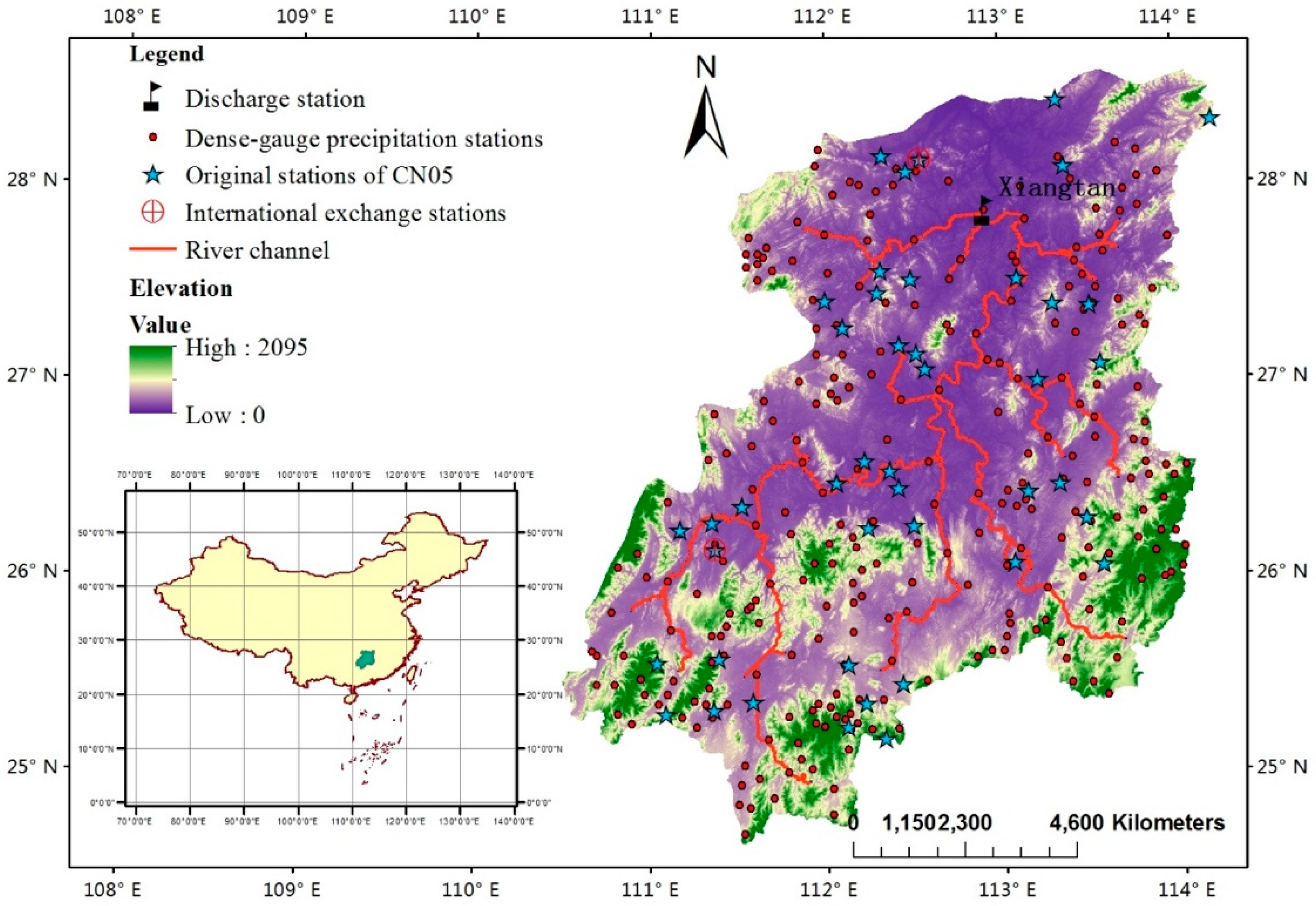
Figure 1. The location of Xiangjiang River Basin and its river channel, precipitation gauge stations (dense-gauge precipitation gauge stations, original stations of CN05, and international exchange stations) and discharge stations.
Remotesensing 12 03550 g001
Figure 2. Mean seasonal precipitation (spring: March–May, summer: June–August, autumn: September–November, winter: December–February, dry season: October–March and wet season: April–September) of 2003–2013 from the dense-gauge precipitation and eight gridded datasets (National Meteorological Information Center dataset from the China Meteorological Administration (CN05), Precipitation Estimation from Remotely Sensed Information Using Artificial Neural Networks (PERSIANN), Climate Prediction Center MORPHing-raw satellite dataset (CMORPH RAW), Tropical Rainfall Measuring Mission (TRMM), PERSIANN Climate Data Record (PERSIANN CDR), CMORPH bias-corrected (CMORPH CRT), CMORPH gauge blended (CMORPH BLD), Multi-Source Weighted-Ensemble Precipitation V2.0 (MSWEP) and Climate Hazards Group InfraRed Precipitation with Stations V2.0 (CHIRPS)).
Remotesensing 12 03550 g002
Figure 3. Summer precipitation (mm) during June–August of 2003–2013 from CN05 and eight satellite-based datasets compared with the dense-gauge dataset, which is shown as colored dots.
Remotesensing 12 03550 g003
Figure 4. Frequency distribution of daily rainfall (A, shown as bar graph), contribution of rain rate classes to the annual accumulation (A, shown as line chart) as well as frequency bias index (FBI), false alarm ratio (FAR), probability of detection (POD), and equitable threat score (ETS) values of the 11-year annual (B,E,H,K), wet season (C,F,I,L), and dry season (D,G,J,M) precipitation process of 2003–2013 on a grid scale for seven daily precipitation thresholds over the Xiangjiang River Basin for the nine gridded datasets (CN05, TRMM, CHIRPS, PERSIANN CDR, CMORPH CRT, CMORPH BLD, MSWEP, PERSIANN and CMORPH RAW) and the dense-gauge dataset.
Remotesensing 12 03550 g004
Figure 5. Relative bias (RB), unbiased root mean squared error (RMSE), and R 2 of the daily precipitation for the nine gridded datasets on both grid (shown as boxplot in (A,C,E)) and watershed (shown as radar plot in (B,D,F)) scales. In radar plots at right sides, red and blue lines represent the optimal values (RB (0), unbiased RMSE (0) and R 2 ( 1 ) ) and the results of gridded datasets of each statistic, respectively.
Remotesensing 12 03550 g005
Figure 6. Annual total precipitation when daily precipitation amount on a wet day > 99th percentile (R99pTOT), the annual daily precipitation amount on a wet day (SDII), and the maximum length of wet and dry spells (CWD and CDD) of the daily precipitation for the nine gridded datasets on both grids (shown as boxplot in (A,C,E,G)) and areal mean (shown as radar plot in (B,D,F,H)) scales. In radar plots at right sides, red line and blue lines respectively represent the results of the dense-gauge dataset and the nine other gridded datasets.
Remotesensing 12 03550 g006
Figure 7. Simulation results of mean monthly hydrographs (2004–2013) using nine gridded datasets and the dense-gauge dataset in the SWAT together with XAJ models.
Remotesensing 12 03550 g007
Figure 8. Boxplot of the relative bias of the daily mean discharge (A), summer high flow (B), and winter low flow (C) simulated using the nine gridded datasets and the dense-gauge dataset based on SWAT (red) together with XAJ (blue) models. Each boxplot is constructed with one value from each year of 2004–2013.
Remotesensing 12 03550 g008
Figure 9. Relative bias of streamflow (A,C,E) and relative bias propagation factor (B,D,F) of the whole year, the wet season and the dry season for the nine gridded datasets based on SWAT (red) together with XAJ (blue) models. Each boxplot is constructed with one value of each year from 2004 to 2013.
Remotesensing 12 03550 g009
Figure 10. Unbiased RMSE of streamflow (A,C,E) and unbiased RMSE propagation factor (B,D,F) of the whole year, the wet season and the dry season for the nine gridded datasets based on SWAT (red) together with XAJ (blue) models. Each boxplot is constructed with one value of each year from 2004–2013.
Remotesensing 12 03550 g010
Table 1. Background information for selected precipitation datasets used in this study.
DatasetCategorySpatial ResolutionTemporal DomainCoverageDeveloperLink
Dense-gaugeGauged267 precipitation stations1963–2013-the Water Conservation Bureau of Hunan Province-
CMAGauge-interpolated0.5° × 0.5°1961–201654°N–18°SChina Meteorological Administrationhttp://data.cma.cn/data
TRMMSatellite-gauge0.25° × 0.25°1998–present50°N–50°SNASA and Japan Aerospace Exploration (JAXA) Agencyftp://trmmopen.gsfc.nasa.gov/pub/merged/3B42RT/
PERSIANN CDR2003-present60°N–60°Sthe Center for Hydrometeorology and Remote Sensing (CHRS) at the University of California, Irvinehttp://chrsdata.eng.uci.edu
CMORPH CRT1998–present50°N–50°SClimate Prediction Center of NOAAftp://ftp.cpc.ncep.noaa.gov/precip/CMORPH_V1.0/CRT/0.25deg-DLY_00Z/
CMORPH BLD1998–present50°N–50°SClimate Prediction Center of NOAAftp://ftp.cpc.ncep.noaa.gov/precip/CMORPH_V1.0/BLD/0.25deg-DLY_EOD/GLB/
CHIRPSBlended1981–present50°N–50°Sthe U.S. Geological Survey (USGS) Earth Resources Observation and Science (EROS) Centerftp://ftp.chg.ucsb.edu/pub/org/chg/products/CHIRPS-2.0
MSWEP1975–present90°N–90°SHylke Beck in Princeton Universityhttp://www.gloh2o.org
PERSIANNSatellite-only2003–present60°N–60°Sthe Center for Hydrometeorology and Remote Sensing (CHRS) at the University of California, Irvinehttp://chrsdata.eng.uci.edu
CMORPH RAW1998–present50°N–50°SClimate Prediction Center of NOAAftp://ftp.cpc.ncep.noaa.gov/precip/CMORPH_V1.0/RAW/0.25deg-DLY_00Z/
Table 2. List of statistical indexes used in this study.
CategoryIndexEquation/DescriptionRange and Optimal Value
Precipitation indicesCategorical statisticsFBI a + b a + c (0, ∞), 1
POD a a + b (0, 1), 1
FAR c a + c (0, 1), 0
ETS a + H e a + b + c H e ( H e = ( a + b ) ( a + c ) N where N is the total number of estimates)(−∞, 1), 1
Quantitative metricsRB i = 1 i = n ( S i G i ) i = 1 i = n G i (− ,   ) , 0
ubRMSE i = 1 n ( G i S i ) 2 n ( i = 1 n ( G i S i ) n ) 2 (0, ∞), 0
R2 [ i = 1 i = n ( G i G ¯ ) ( S i S ¯ ) ] 2 i = 1 i = n ( G i G ¯ ) 2 i = 1 i = n ( S i S ¯ ) 2 (0, 1), 1
Extreme statisticsR99pTOTAnnual total precipitation when daily precipitation amount on a wet day>99th percentile-
SDIIAnnual daily precipitation amount on wet day-
CWDMaximum length of wet spell, maximum number of consecutive days with daily precipitation ≥ 1 mm-
CDDMaximum length of dry spell, maximum number of consecutive days with daily precipitation < 1 mm-
Hydrological indicesEvaluation metricsNSE 1 [ i = 1 n ( Y i o b s Y i s i m ) 2 i = 1 n ( Y i o b s Y ¯ ) 2 ] (−∞, 1), 1
Hydrological statisticsDMDDaily mean discharge-
WLFWinter low flow (5th percentile)-
SHFSummer high flow (95th percentile)-
Error propagation indices γ R B RB   of   runoff RB   of   precipitation (− ,   ) , -
γ u b R M S E ubRMSE   of   runoff ubRMSE   of   precipitation (0, ∞), -
Table 3. Comparison of Nash–Sutcliffe efficiency (NSE) of both Xinanjiang (XAJ) and Soil and Water Assessment Tool (SWAT) models in daily step simulation based on the dense-gauge and the nine precipitation datasets.
DatasetsPeriodXAJ
NSE
SWAT
NSE
Dense-gaugeCalibration (2004–2010)0.890.86
Validation (2011–2013)0.890.84
CN05(2004–2013)0.860.83
PERSIANN−0.4−0.31
CMORPH RAW−0.97−0.95
TRMM0.730.72
PERSIANN CDR0.560.58
CMORPH CRT0.750.73
CMORPH BLD0.840.81
MSWEP0.780.79
CHIRPS0.440.48
Publisher’s Note: MDPI stays neutral with regard to jurisdictional claims in published maps and institutional affiliations.