Abstract
Plane fitting is a fundamental operation for point cloud data processing. Most existing methods for point cloud plane fitting have been developed based on high-quality Lidar data giving equal weight to the point cloud data. In recent years, using low-quality RGB-Depth (RGB-D) sensors to generate 3D models has attracted much attention. However, with low-quality point cloud data, equal weight plane fitting methods are not optimal as the range errors of RGB-D sensors are distance-related. In this paper, we developed an accurate plane fitting method for a structured light (SL)-based RGB-D sensor. First, we derived an error model of a point cloud dataset from the SL-based RGB-D sensor through error propagation from the raw measurement to the point coordinates. A new cost function based on minimizing the radial distances with the derived rigorous error model was then proposed for the random sample consensus (RANSAC)-based plane fitting method. The experimental results demonstrated that our method is robust and practical for different operating ranges and different working conditions. In the experiments, for the operating ranges from 1.23 meters to 4.31 meters, the mean plane angle errors were about one degree, and the mean plane distance errors were less than six centimeters. When the dataset is of a large-depth-measurement scale, the proposed method can significantly improve the plane fitting accuracy, with a plane angle error of 0.5 degrees and a mean distance error of 4.7 cm, compared to 3.8 degrees and 16.8 cm, respectively, from the conventional un-weighted RANSAC method. The experimental results also demonstrate that the proposed method is applicable for different types of SL-based RGB-D sensor. The rigorous error model of the SL-based RGB-D sensor is essential for many applications such as in outlier detection and data authorization. Meanwhile, the precise plane fitting method developed in our research will benefit algorithms based on high-accuracy plane features such as depth calibration, 3D feature-based simultaneous localization and mapping (SLAM), and the generation of indoor building information models (BIMs).
1. Introduction
Point cloud datasets are widely used for 3D model generation [1,2], high definition (HD) map generation [3,4,5], and robot/vehicle navigation [6,7]. Instead of directly using millions of points in the point cloud, 3D modeling is an important step to organize point cloud data [8], and fitting the point cloud to regular shapes (e.g., plane, cylinder, and sphere) is crucial for point cloud classification and segmentation [9,10].
Currently, point cloud datasets are mainly generated by a terrestrial laser scanner (TLS) or an RGB camera. TLS can collect point cloud data with a high accuracy of up to the millimeter-level. However, the high cost and long field surveying time of TLS restrict the broad applications of this technology [11]. Instead, by using an RGB camera, the hardware cost and data collection time can be significantly reduced, but the transformation from color images to a 3D point cloud requires a substantial computation cost and extra scale control. In addition, the output point cloud generally has low precision and reliability [12].
The RGB-D sensor is another choice for point cloud collection, which provides both color images and dense depth maps [13]. According to the principle of range measurements, RGB-D sensors can be divided into two categories: time-of-flight (ToF)-based and structured light (SL)-based sensors [14]. To date, there are numerous RGB-D sensors on the market such as the Xtion Pro from Asus (2012), the second-generation Kinect from Microsoft (2013), Structure Sensor (2014), and the RealSense Series from Intel (2015). Although they were first introduced for the game industry where the accuracy of the measurements is not crucial, RGB-D sensors have been applied for many high accuracy applications recently, for example, indoor 3D modeling [15], simultaneous localization and mapping (SLAM) [16], and augmented reality applications [17], etc., in which the rigorous calibration and error modeling of RGB-D sensor data become increasingly essential [18].
For the 3D modeling of point cloud data, the extraction of regular shapes (i.e., plane, sphere, and cylinder) from point coordinates is an important step for the usage of the point cloud. For example, many studies have tried to develop plane fitting methods for depth calibration [19,20], object segmentation [9,10], and 3D environment reconstruction [21,22,23]. In general, the plane estimation algorithms of the point cloud can be divided into three groups. The first group is based on the classical least-squares (LS) [24,25], which estimates the plane parameters by minimizing the squared offset between the plane and the candidate points. This method performs well for a dataset with few outliers, for example, those collected by the high-performance TLS. However, the performance of this type of method can be significantly degraded if the data quality is low and has a large portion of outliers, or the occlusion region is considerably large [20]. The second group is based on feature space transformations such as principal component analysis (PCA) [26,27] and Hough transform (HT) [14,28]. Nevertheless, PCA is also sensitive to the outliers in a similar way to LS, while HT requires extensive computation and rigorous accumulator design. Therefore, these methods are also difficult to apply to low-quality point cloud data.
The third group is the RANSAC-based fitting methods [29,30], which can provide robust fitting with noisy datasets. This method is a minimization algorithm, as with LS, but the iterations with candidate plane generation by randomly picking a few points dramatically overcome the noise-sensitive problem. Furthermore, M-estimator sample consensus (MLESAC) [31] and progressive sample consensus (PROSAC) [32] have been developed based on the maximum likelihood estimation, which improves the robustness of the RANSAC methods. These plane fitting methods based on RANSAC are useful and practical for high-quality Lidar data. However, there are still some shortcomings in handling datasets collected by a low-cost RGB-D sensor, since the noises of the measurements are significantly larger and distance-related.
Recently, many works have been undertaken to address the plane fitting issue of low-quality point clouds collected by a low-cost RGB-D sensor. Holz et al. [33] proposed smoothing the points with multilateral filtering and model the camera noise with a distance-related empirical model. The experimental results demonstrated that this method achieved excellent performance in the extraction of planes and the image segmentation with a dataset collected by Kinect. However, this method is impractical and ineffective because it requires the generation of an individual model for the particular hardware and applied environment. Fuersattel et al. [34] integrated the fitting of regular shapes with sensor calibration by applying a precise plane fitting method based on the least-squares and improved the accuracy significantly with angle errors of less than a degree and distance errors less than 2 cm. Additionally, their research indicated that the error of the SL-based RGB-D sensor was distance-related, and that the performance of the plane fitting algorithm will decrease as the operating range increases. However, they only tested an algorithm with the dataset in a very close operation range (less than 1.7 meters), where there is relatively little noise. The considerable error in the extended operating range and the vast depth measurement scale in the same frame will be challenging for this method.
In this paper, an improved plane-fitting algorithm, based on the standard RANSAC framework, was proposed to address this issue. First, we derived a rigorous error model for the SL-based RGB-D sensor based on its working principle and error propagation law, from which the weighted coordinates of each point were established. Then, we proposed using the radial distance—that is, the distance in the ray direction—to calculate the residuals for plane estimation by adopting the error characteristics of the SL depth sensors. Next, we modified the cost function of the standard RANSAC with residuals along the radial direction and the weighting information. The experiments and discussions are given in Section 4, while the conclusions are presented in Section 5.
2. Error Distribution of SL Depth Sensors
In this section, we present the working principle of an SL-based RGB-D sensor and discuss the factors that contribute to the error of depth measurements.
An SL-based depth sensor consists of an infrared projector and an infrared camera. The depth for each pixel in the scene is computed from the disparity value, which is the difference between the predesigned pattern emitted from the infrared projector and the actual pattern recorded by the infrared camera. The principle of the SL-based depth sensor is illustrated in Figure 1.
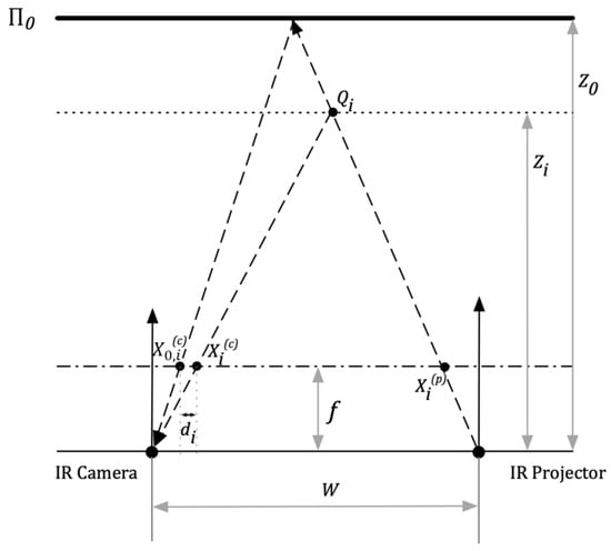
Figure 1.
Work principle of structured light (SL)-based depth sensor.
Assume that a pattern is projected in the direction of point onto the reference plane with a distance , and reflected to the infrared camera at the 2D position ; we can obtain
where is the distance between the camera and the projector; indicates the focal length of the infrared camera; and represents the distance between the plane and the sensor.
If the real reflected target is at the point , and the pattern is recorded at on the infrared camera image, the disparity is then defined as
and the coordinates of the point can be obtained as [18]
For most SL-based depth sensors, the output is a normalized disparity with values from 0 to 2047, and the disparity is calculated using
where and are two coefficients. Therefore, the distance can be rewritten as
where , which can be estimated through the calibration of the sensor [18]. The quality of the depth depends on the accuracy of the disparity . The error function of disparity can be expressed as:
where is the measurement value of disparity; denotes the actual value of disparity; and and represent the system error and the measurement noise, respectively. All the values in Equation (6) reference the pixel unit. Inserting Equation (4) into Equation (6), the normalized disparity can be described as
where is the measurement of normalized disparity; indicates the actual value of normalized disparity; denotes the normalized system error; and is the normalized measurement noise.
Based on the Brown model [35] and the work in [18,36], the systematic error can therefore be modeled as
where are the parameters to model the tangential distortion; represent the parameters to model the radial distortion; is the coordinate of the image point; and .
Then, the Taylor series is used to present Equation (5), with the linear term as
where is the expansion point. Considering that the measurement noise is in a normal distribution with a variance , the variance of can be calculated based on the error propagation law:
By combining Equation (3) and Equation (10), the variances of measurement point coordinates () are
3. Modified RANSAC Algorithm
In this section, we present the algorithm used in this research and give a detailed description of the proposed method.
As Figure 2 shows, the workflows of the RANSAC plane fitting algorithm can be summarized as follows:
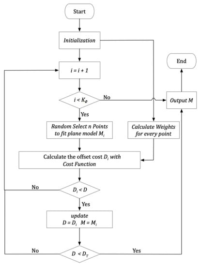
Figure 2.
Workflow of the modified plane fitting algorithm based on random sample consensus (RANSAC).
- Initialize the program with input point cloud and iteration limit ;
- Select points randomly from point cloud to generate the candidate plane model ;
- Calculate the mean offset between each point in point cloud and the candidate plane model based on a cost function;
- Update the best fitting plane model and the corresponding mean offset ;
- Repeat steps 1–4 until the iteration number is larger than the iteration limit or the value of is smaller than the threshold (in this paper, ).
The value of the iteration limit is calculated as [37]
where is the desired probability for the algorithm to provide an acceptable result; denotes the probability to choose an inlier each time a point is selected; and is the number of points to generate the candidate plane. Considering the quality of the dataset [37], here, we use , and .
Using seriously corrupted data, the methods based on RANSAC provide not only estimation results in a shorter time, but also with higher reliability, compared to the methods based on LS and feature space transformations [38]. However, there are still some problems with handling the dataset from low-cost RGB-D sensors. First, as Figure 3a shows, in the standard RANSAC-based methods, the perpendicular distance is commonly used to evaluate the accuracy of the plane fitting result, which assumes the error distribution of every point in the point cloud is isotropic and comparable [37,38]. This situation is applicable for a high-quality TLS dataset, because the error is ignorable, especially for plane fitting. Nevertheless, this would be problematic for low-cost RGB-D sensors, since the datasets are much noisier, and the error distribution is anisotropic and heterogeneous. Alternatively, the distance along one given coordinate axis such as the normal direction distance shown in Figure 3b, has been widely used in LS-based methods [39]. However, nearly all algorithms based on this criterion strongly depend on the coordinate system. Second, standard RANSAC ignores the fact that the contributions of points with different quality should be different for the candidate plane evaluation. Moreover, this fact happens to be the critical point for the plane estimation of a low-quality dataset, considering that the noisy points frequently deflect the candidate plane from the correct position.
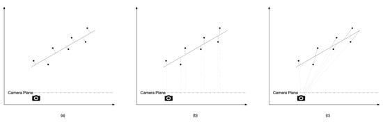
Figure 3.
Residuals in different directions: (a) perpendicular direction, (b) camera’s plane normal direction, (c) radial direction.
As shown in Equation (3), the and coordinates of each measured point are calculated based on the measured depth and the image coordinate . This means that if is fixed, for any depth measurement, the 3D point corresponding to will always be located on the radial direction line that starts from the camera origin and passes the image point . Therefore, in the 3D space, the measurement error of the SL-based RGB-D sensor is in the radial direction, as illustrated in Figure 4, in which the red point is the measured point, the black point is the object point, and the measurement error is the distance between the measured and the object point.
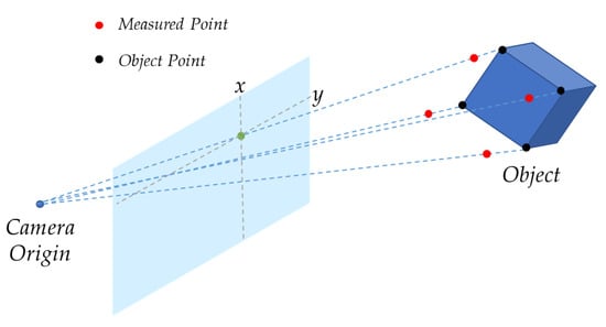
Figure 4.
Three-dimensional ranging error presentation of the SL-based RGB-D sensor.
In this paper, we modified the traditional RANSAC algorithm by replacing the perpendicular distance with the radial distance. The candidate plane model in the 3D space is expressed as , where is the normal unit vector of the plane, with the condition as . is the perpendicular distance between the coordinate system origin and the plane. In this way, the problem of plane fitting could be formulated as the estimation of and . As Figure 5 shows, the radial direction offset between one arbitrary point and the detected candidate plane can be written as
where is the location of the camera center , and illustrates the intersection point between the radial line and the detected plane. If we set to the original point of the coordinate system, can be calculated as
where is the focal length of the Infrared (IR) camera and is the pixel local of the measurement point. By integrating Equations (10), (13), and (14), we can obtain the variance of :
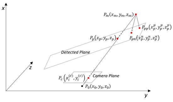
Figure 5.
Illustration of the offset calculation. is the offset in the perpendicular direction is the offset in the camera plane normal direction, and is the offset in the radial direction.
We then set up the cost function based on the points weighted by Equation (15). For each iteration, the weighted mean offset in the radial direction is expressed as
where is the index of the point; denotes the variance of ; is the location of point ; and indicates the intersection point of the detected plane and the radial line.
Similarly, the cost function using an offset in the perpendicular direction can be written as
where is the intersection point of the detected plane and its perpendicular line through point . The cost function using an offset in the direction of the camera plane normal is
where is the intersection point of the detected plane and the line through point , which is parallel to the normal direction of the camera plane. The cost function using an offset without weight information in the radial direction is
The output plane parameters are then determined by minimizing the value of for all iterations, or under the case that the value of is smaller than the threshold .
4. Experiments and Results
In this section, we present the design of the experiments and discuss the results. Three series of experiments have been done to evaluate the performance of the proposed method.
To quantify the accuracy of the planes fitted with different cost functions, the angle error , the difference of , and the mean offset of control points compared to the “true plane” are used as metrics for comparison:
where is the normal unit vector of the ground truth plane that equals ; is the normal unit vector of the estimated plane that equals ; denotes the perpendicular distance between the origin of the camera coordinate system and the ground truth plane; represents the perpendicular distance between the origin of the camera coordinate system and the estimated plane; indicates the number of control points; illustrates the “true” position of control points; and is the position of points in the estimated plane corresponding to the control points.
4.1. Experiment for Different Operating Ranges
The first experiment was designed to test whether the proposed method is practical for different operating ranges. As shown in Figure 6, the RGB-D sensor used in this experiment was the Structural Sensor [40], which can be fitted to an iPad, an iPhone, or other mobile instruments. First, the distortion error of the IR camera was calibrated using the method proposed in [36]. Table 1 gives the calibration parameters for both radial and tangential distortions.
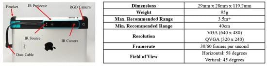
Figure 6.
The main elements of hardware used in this paper, which includes one RGB-D camera and one iPad [40].

Table 1.
Parameters for system error calibration.
The effect of the calibration is demonstrated in Figure 7, where the projected point clouds of a plane wall for both uncalibrated and calibrated systems are plotted. The improvement in the calibrated depth can be clearly seen as the wall should be a straight line after projection to the floor. Additionally, the quantitative analysis of the depth calibration in the different operating ranges and different areas of the frame is shown in Figure 8. The illustration of the center area and edge area is shown in Figure 9. The accuracy of the depth measurement improved significantly with the calibration operation, especially for the far range and edge area.
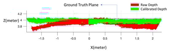
Figure 7.
Comparison of real data from the Structural Sensor and simulation data based on the distortion error model.
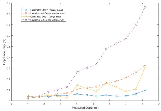
Figure 8.
Quantitative analysis of the depth calibration.
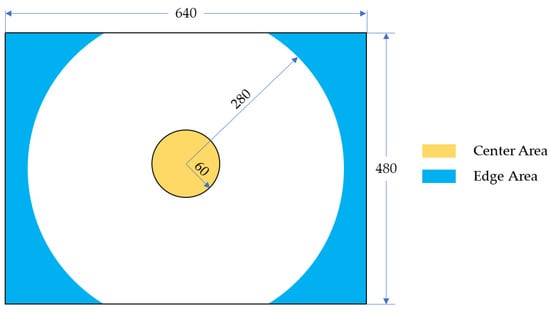
Figure 9.
Illustration of the center and edge area; all values are in pixel units.
The test field and the equipment setup for the data collection are shown in Figure 10. The identifiable control points with known coordinates were distributed on the wall plane with the ground truth obtained by the total station. In our test, the dataset was captured at three different ranges—close range (1.23 m), middle range (2.47 m), and far range (4.31 m)—while the camera was arranged substantially parallel to the wall plane. Then, different cost functions, as discussed in Section 3, were used to fit the wall plane. The “true plane” parameters were obtained from the surveyed coordinates of the control points.
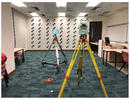
Figure 10.
Test field and equipment setup for the first experiment.
For each operating range, we captured 20 datasets for evaluation. Table 2 shows the mean values of the metrics and the standard deviation for the different cost functions and operating ranges. The performances of the perpendicular-based and normal-based method were similar because their values are approximate when the camera plane is parallel to the observed wall plane. For the close range and middle range, when the error of a point in the edge area is not very large, the radial-based method is practical to refine the plane fitting result in terms of both angle and distance, but it is not helpful for the far range because this type of error is distance-related. However, our proposed method, using the radial offset and the weighted cost function, demonstrated higher robustness and is practicable for all three test datasets. In particular, this method reduced the angle error by about one degree. The reason for this is that the weighted cost function mitigates the influence of noisy points. Considering that the noise and error of the depth measurement increases with the operating range, this experiment also demonstrated that the proposed method is effective and practical for datasets with different levels of noise and error.
Table 2.
Mean value of metrics for the different operating ranges. LS: least-squares.
4.2. Experiment for Large Depth Measurement Scales
The second experiment was designed to test the performance of the proposed method with the dataset in a large depth measurement scale. As above-mentioned, the error of the SL-based RGB-D sensor will increase exponentially with the ranging distance. The points close to the equipment and in the center area of the depth image always exhibit small errors, while the points far from the equipment and in the edge area of the depth image always display a significant error (Figure 11). This issue is challenging for the unweighted method because the error distribution of the dataset is asymmetrical.
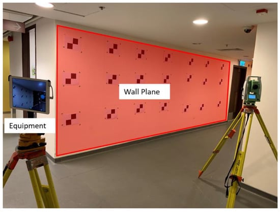
Figure 11.
Test field and equipment setup for the second experiment.
As Figure 11 shows, the basic setup of this experiment was like the first experiment. Notably, a flat wall with a height of 2.4 m and a width of 6.4 m was used as the test area, while the coordinates of the control points were surveyed using a total station with an accuracy at the millimeter-level. Then, different cost functions, as discussed in Section 3, were used to fit the wall plane. There were 62 control points on the wall (Figure 12a), and the depth measurements of the control points were in the range of 3.5 m to 7.5 m (Figure 12b).
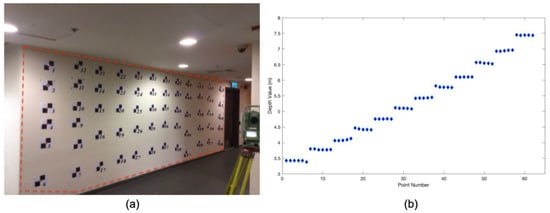
Figure 12.
(a) Test area of the plane fitting experiment, (b) true depth value of the control points.
The conventional plane fitting method minimizing the sum of perpendicular distance was used as the baseline during the comparison. For each cost function, 20 datasets were collected, and the mean values of metrics as well as the standard deviation are given in Table 3. We observed that the cost function with weighted radial distance reduced the plane fitting errors dramatically to 0.5 degrees of angle error and 4.7 cm of range error, compared to 2 to 4 degrees of angle error and 12 to 16 cm of range error when the unweighted cost functions were used.
Table 3.
Mean value of metrics for the second experiment.
Figure 13 shows the 3D views of the fitted planes with different cost functions. It is clear that the plane, by minimizing the weighted radial residual (red area) proposed in this study, was one closer to the true plane (green area).
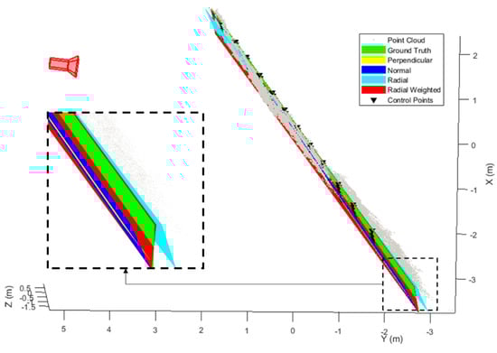
Figure 13.
Qualitative results of the different plane fitting methods.
The errors of the control points after plane fitting calibration based on different methods are illustrated in Figure 14. Compared with Figure 6b, which gives the range of control points, the errors for the raw data and unweighted cost functions are range-related. The longer the operating range, the larger the error. With the help of the weighted plane fitting method, the range errors were controlled to an accuracy of better than 0.1 m for all of the distance ranges (3.5 m to 7.5 m).
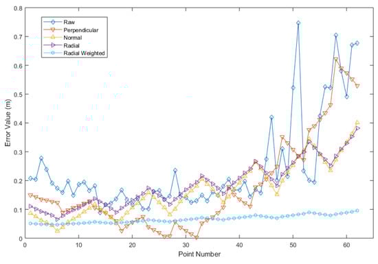
Figure 14.
The errors of the control points after plane fitting calibration.
4.3. Experiment with Kinect V2
The third experiment was designed to evaluate the applicability of the proposed method for different types of SL-based RGB-D sensor. In this experiment, we used the Kinect v2 to collect the sample data under a similar test condition to the second experiment. The test results are shown in Table 4. When compared to the unweighted perpendicular-based method, the proposed method improved the accuracy of the plane fitting significantly, with the angle error improving from 2.7 degrees to 0.9 degrees and the distance error from 15.5 cm to 7.1 cm. This experiment indicates that the proposed method is practical for different types of SL-based RGB-D sensors.
Table 4.
Mean values of the metrics for the third experiment.
5. Conclusions
Fitting point cloud data to regular shapes (i.e., plane, sphere, and cylinder) is a fundamental step for point cloud classification, segmentation, and calibration. For low-cost RGB-D sensors, since the depth measurements are range-related, any unweighted fitting methods will introduce significant errors in the fitted shapes.
In this paper, we derived a rigorous error model for a point cloud dataset generated by a low-cost SL-based RGB-D sensor. Based on this error model, we proposed a novel RANSAC-based plane fitting method by replacing the cost function of the perpendicular offset to the weighted radial offset. The experimental results showed that our proposed method is robust and practical for different operating ranges, different working conditions, and different types of SL-based RGB-D sensors. For operating ranges between 1.23 meters and 4.31 meters, the proposed method can obtain a plane fitting result with an angle error of about one degree and a distance error less than 6 cm. Meanwhile, the proposed method improved the angle accuracy from 3.8 degrees to 0.5 degrees and the distance error from 16.8 centimeters to 4.7 centimeters, compared to the unweighted perpendicular offset cost function, with a dataset in a large depth measurement scale.
Further research is still required to apply the proposed error model to the fitting algorithm of more complex shapes (e.g., sphere, cylinder, and curved surfaces). We will also use this point weighting method to identify the confidence of the point matching results of the RGB-D-based SLAM system to improve the robustness and accuracy of the SLAM system. These shape data and precise 3D point clouds will be used to establish an automatic indoor BIM generation system.
Author Contributions
Conceptualization, Y.L.; Methodology, Y.L., W.L., and W.D.; Software, Y.L., W.L., W.D., and S.T.; Validation, Y.L., W.L., and Y.H.; Formal analysis, Y.L. and W.L.; Data curation, Y.L. and Y.H.; Supervision, W.C.; Writing—original draft preparation, Y.L.; Writing—review and editing, W.C. and Y.L. All authors have read and agreed to the published version of the manuscript.
Acknowledgments
The research was substantially funded by the Shenzhen Science and Technology Innovation Commission (Project No. JCYJ20170818104822282), Hong Kong Research Grants Council (RGC) Competitive Earmarked Research Grant (Project No: 152223/18E), and the research fund from the Research Institute of Sustainable Urban Development, The Hong Kong Polytechnic University.
Conflicts of Interest
The authors declare no conflicts of interest.
References
- Dorninger, P.; Pfeifer, N. A comprehensive automated 3D approach for building extraction, reconstruction, and regularization from airborne laser scanning point clouds. Sensors 2008, 8, 7323–7343. [Google Scholar] [CrossRef] [PubMed]
- Wang, C.; Cho, Y.K.; Kim, C. Automatic BIM component extraction from point clouds of existing buildings for sustainability applications. Autom. Constr. 2015, 56, 1–13. [Google Scholar] [CrossRef]
- Patra, S.; Bhowmick, B.; Banerjee, S.; Kalra, P. High Resolution Point Cloud Generation from Kinect and HD Cameras using Graph Cut. VISAPP 2012, 12, 311–316. [Google Scholar]
- Seif, H.G.; Hu, X.J.E. Autonomous driving in the iCity-HD maps as a key challenge of the automotive industry. Engineering 2016, 2, 159–162. [Google Scholar] [CrossRef]
- Yang, B.; Liang, M.; Urtasun, R. Hdnet: Exploiting hd maps for 3d object detection. In Proceedings of the Conference on Robot Learning, Osaka, Japan, 30 October–1 November 2019; pp. 146–155. [Google Scholar]
- Biswas, J.; Veloso, M. Depth camera based indoor mobile robot localization and navigation. In Proceedings of the 2012 IEEE International Conference on Robotics and Automation, Saint Paul, MN, USA, 14–18 May 2012; pp. 1697–1702. [Google Scholar]
- Whitty, M.; Cossell, S.; Dang, K.S.; Guivant, J.; Katupitiya, J. Autonomous navigation using a real-time 3d point cloud. In Proceedings of the Australasian Conference on Robotics and Automation, Brisbane, Australia, 1–3 December 2010; pp. 1–3. [Google Scholar]
- Wang, C.; Tanahashi, H.; Hirayu, H.; Niwa, Y.; Yamamoto, K. Comparison of local plane fitting methods for range data. In Proceedings of the 2001 IEEE Computer Society Conference on Computer Vision and Pattern Recognition, Kauai, HI, USA, 8–14 December 2001; Institute of Electrical and Electronics Engineers (IEEE): Piscataway, NJ, USA; pp. 663–669. [Google Scholar]
- Kim, K.; Davis, L.S. Multi-Camera tracking and segmentation of occluded people on ground plane using search-Guided particle filtering. In Proceedings of the 9th European Conference on Computer Vision, Graz, Austria, 7–13 May 2006; pp. 98–109. [Google Scholar]
- Trevor, A.J.; Gedikli, S.; Rusu, R.B.; Christensen, H.I. Efficient Organized Point Cloud Segmentation with Connected Components. In Proceedings of the 3rd Workshop on Semantic Perception Mapping and Exploration (SPME), Karlsruhe, Germany, 5 May 2013. [Google Scholar]
- Volk, R.; Stengel, J.; Schultmann, F. Building Information Modeling (BIM) for existing buildings-Literature review and future needs. Autom. Constr. 2014, 38, 109–127. [Google Scholar] [CrossRef]
- Henry, P.; Krainin, M.; Herbst, E.; Ren, X.; Fox, D. RGB-D mapping: Using Kinect-Style depth cameras for dense 3D modeling of indoor environments. Int. J. Robot. Res. 2012, 31, 647–663. [Google Scholar] [CrossRef]
- Han, J.; Shao, L.; Xu, D.; Shotton, J. Enhanced computer vision with microsoft kinect sensor: A review. IEEE Trans. Cybern. 2013, 43, 1318–1334. [Google Scholar]
- Hulik, R.; Spanel, M.; Smrz, P.; Materna, Z. Continuous plane detection in point-Cloud data based on 3D Hough Transform. J. Vis. Commun. Image Represent. 2014, 25, 86–97. [Google Scholar] [CrossRef]
- Tang, S.; Zhu, Q.; Chen, W.; Darwish, W.; Wu, B.; Hu, H.; Chen, M. Enhanced RGB-D mapping method for detailed 3D indoor and outdoor modeling. Sensors 2016, 16, 1589. [Google Scholar] [CrossRef]
- Sturm, J.; Engelhard, N.; Endres, F.; Burgard, W.; Cremers, D. A benchmark for the evaluation of RGB-D SLAM systems. In Proceedings of the 2012 IEEE/RSJ International Conference, Intelligent Robots and Systems (IROS), Algarve, Portuga, 7–12 October 2012; pp. 573–580. [Google Scholar]
- Newcombe, R.A.; Izadi, S.; Hilliges, O.; Molyneaux, D.; Kim, D.; Davison, A.J.; Kohi, P.; Shotton, J.; Hodges, S.; Fitzgibbon, A. KinectFusion: Real-Time dense surface mapping and tracking. In Proceedings of the 2011 10th IEEE International Symposium, Mixed and Augmented Reality (ISMAR), Basel, Switzerland, 26–29 October 2011; pp. 127–136. [Google Scholar]
- Darwish, W.; Tang, S.; Li, W.; Chen, W. A new calibration method for commercial RGB-d sensors. Sensors 2017, 17, 1204. [Google Scholar] [CrossRef]
- Chai, Z.; Sun, Y.; Xiong, Z. A Novel Method for LiDAR Camera Calibration by Plane Fitting. In Proceedings of the IEEE/ASME International Conference on Advanced Intelligent Mechatronics (AIM), Auckland, New Zealand, 9–12 July 2018; pp. 286–291. [Google Scholar]
- Xu, L.; Au, O.C.; Sun, W.; Li, Y.; Li, J. Hybrid plane fitting for depth estimation. In Proceedings of the 2012 Asia-Pacific, Signal & Information Processing Association Annual Summit and Conference (APSIPA ASC), Hollywood, CA, USA, 3–6 December 2012; pp. 1–4. [Google Scholar]
- Habbecke, M.; Kobbelt, L. Iterative multi-View plane fitting. In Proceedings of the International Fall Workshop of Vision, Modeling, and Visualization, Aachen, Germany, 22–24 November 2006; pp. 73–80. [Google Scholar]
- Habbecke, M.; Kobbelt, L. A surface-Growing approach to multi-View stereo reconstruction. In Proceedings of the IEEE Conference on Computer Vision and Pattern Recognition, Minneapolis, MN, USA, 17–22 June 2007; pp. 1–8. [Google Scholar]
- Xu, K.; Huang, H.; Shi, Y.; Li, H.; Long, P.; Caichen, J.; Sun, W.; Chen, B. Autoscanning for coupled scene reconstruction and proactive object analysis. ACM Trans. Graph. (TOG) 2015, 34, 177. [Google Scholar] [CrossRef]
- Chen, Y.; Medioni, G. Object modelling by registration of multiple range images. Image Vis. Comput. 1992, 10, 145–155. [Google Scholar] [CrossRef]
- Hong, L.; Chen, G. Segment-Based stereo matching using graph cuts. In Proceedings of the 2004 IEEE Computer Society Conference on Computer Vision and Pattern Recognition, Washington, DC, USA, 27 June–2 July 2004; pp. 74–81. [Google Scholar]
- Oniga, F.; Nedevschi, S. Processing dense stereo data using elevation maps: Road surface, traffic isle, and obstacle detection. IEEE Trans. Veh. Technol. 2010, 59, 1172–1182. [Google Scholar] [CrossRef]
- Pearson, K. LIII. On lines and planes of closest fit to systems of points in space. Lond. Edinb. Dublin Philos. Mag. J. Sci. 1901, 2, 559–572. [Google Scholar] [CrossRef]
- Borrmann, D.; Elseberg, J.; Lingemann, K.; Nüchter, A. The 3d hough transform for plane detection in point clouds: A review and a new accumulator design. 3D Res. 2011, 2, 3. [Google Scholar] [CrossRef]
- Bolles, R.C.; Fischler, M.A. A RANSAC-Based Approach to Model Fitting and Its Application to Finding Cylinders in Range Data. In Proceedings of the International Joint Conference on Artificial Intelligence, Macao, China, 10–16 August 2019; pp. 637–643. [Google Scholar]
- Sande, C.V.D.; Soudarissanane, S.; Khoshelham, K. Assessment of relative accuracy of AHN-2 laser scanning data using planar features. Sensors 2010, 10, 8198–8214. [Google Scholar] [CrossRef]
- Chum, O.; Matas, J. Matching with PROSAC-Progressive sample consensus. In Proceedings of the IEEE Computer Society Conference on Computer Vision and Pattern Recognition, San Diego, CA, USA, 20–25 June 2005; pp. 220–226. [Google Scholar]
- Torr, P.H.; Zisserman, A. MLESAC: A new robust estimator with application to estimating image geometry. Comput. Vis. Image Underst. 2000, 78, 138–156. [Google Scholar] [CrossRef]
- Holz, D.; Behnke, S. Approximate triangulation and region growing for efficient segmentation and smoothing of range images. Robot. Auton. Syst. 2014, 62, 1282–1293. [Google Scholar] [CrossRef]
- Fuersattel, P.; Placht, S.; Maier, A.; Riess, C. Geometric primitive refinement for structured light cameras. Mach. Vis. Appl. 2018, 29, 313–327. [Google Scholar] [CrossRef]
- Heikkila, J.; Silven, O. A four-Step camera calibration procedure with implicit image correction. In Proceedings of the Conference on Computer Vision and Pattern Recognition, San Juan, Puerto Rico, USA, 17–19 June 1997; p. 1106. [Google Scholar]
- Darwish, W.; Li, W.; Tang, S.; Wu, B.; Chen, W. A Robust Calibration Method for Consumer Grade RGB-D Sensors for Precise Indoor Reconstruction. IEEE Access 2019, 7, 8824–8833. [Google Scholar] [CrossRef]
- Schnabel, R.; Wahl, R.; Klein, R. Efficient RANSAC for point-Cloud shape detection. Comput. Graph. Forum 2007, 26, 214–226. [Google Scholar] [CrossRef]
- Li, L.; Yang, F.; Zhu, H.; Li, D.; Li, Y.; Tang, L. An improved RANSAC for 3D point cloud plane segmentation based on normal distribution transformation cells. Remote Sens. 2017, 9, 433. [Google Scholar] [CrossRef]
- Miyagawa, S.; Yoshizawa, S.; Yokota, H. Trimmed Median PCA for Robust Plane Fitting. In Proceedings of the 25th IEEE International Conference on Image Processing (ICIP), Athens, Greece, 7–10 October 2018; pp. 753–757. [Google Scholar]
- Occipital. Structure Sensor. Available online: https://structure.io/structure-sensor (accessed on 5 December 2019).


© 2020 by the authors. Licensee MDPI, Basel, Switzerland. This article is an open access article distributed under the terms and conditions of the Creative Commons Attribution (CC BY) license (http://creativecommons.org/licenses/by/4.0/).