A LSTM Algorithm Estimating Pseudo Measurements for Aiding INS during GNSS Signal Outages

Abstract

Aiming to improve the navigation accuracy during global navigation satellite system (GNSS) outages, an algorithm based on long short-term memory (LSTM) is proposed for aiding inertial navigation system (INS). The LSTM algorithm is investigated to generate the pseudo GNSS position increment substituting the GNSS signal. Almost all existing INS aiding algorithms, like the multilayer perceptron neural network (MLP), are based on modeling INS errors and INS outputs ignoring the dependence of the past vehicle dynamic information resulting in poor navigation accuracy. Whereas LSTM is a kind of dynamic neural network constructing a relationship among the present and past information. Therefore, the LSTM algorithm is adopted to attain a more stable and reliable navigation solution during a period of GNSS outages. A set of actual vehicle data was used to verify the navigation accuracy of the proposed algorithm. During 180 s GNSS outages, the test results represent that the LSTM algorithm can enhance the navigation accuracy 95% compared with pure INS algorithm, and 50% of the MLP algorithm.

1. Introduction

The inertial navigation system (INS) and global navigation satellite system (GNSS) are two of the main and most important approaches for providing position and attitude information for geographical references [1]. The INS has high accuracy in a short period of time not affected by the environment. However, a standalone INS solution will degrade over time, because of the large errors in the raw measurements of inertial measurement units (IMU) [2]. In this study, the signal from GNSS is adopted to provide high precision navigation solutions. Under decent visibility conditions, GNSS can provide continuous and accurate navigation information over a long period of time. However, GNSS alone cannot give reliable positions all of the time, as the satellite signal may be blocked or corrupted as a result of high buildings, viaducts, tunnels, mountains, multi-path reflections, and bad weather conditions [3,4,5]. Because of their complementary properties, INS and GNSS are commonly integrated by a Kalman filter (KF) for providing continuous and high precision navigation [3,4,5,6]. In an INS/GNSS system, GNSS aids INS by estimating its errors in KF [7,8]. Besides, INS connects the GNSS signal gap and helps the GNSS signal reacquisition after an outage [9,10]. However, when the GNSS signal is blocked, KF cannot update information from the GNSS measurements. Meanwhile, the INS/GNSS system changes into a pure mode, whose position error will diverge over a period of time [2,3,4,11]. Therefore, an improved fusion algorithm needs to be explored so as to improve the INS navigation performance when the GNSS signal is lost.

With the development of artificial intelligence (AI) and big data, a lot of AI methods have been explored so as to improve navigation accuracy during GNSS outages [12,13,14,15,16,17,18]. Nowadays, artificial neural networks (ANN) are the most widely used methods to model a complex nonlinear problem. Many researchers have built a variety of neural networks for aiding INS when the GNSS signal is lost. Rashad and his team first used a radial basis function neural network to model the INS position and the position error between INS and GNSS [12,13]. EI-Sheimy used time, velocity, and yaw as inputs to model the position error and velocity, showing a more stable and accurate result [14]. In later works, an improved autoregressive delay-dependent neural network model was applied. The input features are the current and past one-step position and velocity from IMU and INS, while the output is the INS position error $\delta P_{INS}$ [15]. Another method based on the ensemble model has been explored to promote the generalization of the algorithm by utilizing a lot of weak learners to construct a strong learner [7,15,17]. Furthermore, the support vector machine and genetic algorithm were also explored so as to overcome the over-fitting and local-minimum problems of neural networks [18]. Lately, factor graph optimizations have been widely used for multi-sensor fusion in autonomous systems [19]. This method uses a factor graph model to represent the joint probability distribution function. An efficient incremental inference algorithm over the factor graph is applied, which yields a near-optimal inertial navigation system.

However, almost all of the above methods are based on a static neural network, like the radial basis function neural network (RBF) or multilayer perceptron neural network (MLP). The conception of all above approaches is to model the current and past one-step INS information by training the AI model when the GNSS signal is available. Almost all of the existing INS aiding algorithms try to improve the navigation solutions during GNSS outages by predicting the INS errors using previous INS outputs. The major drawback of which is that they cannot store more past vehicle dynamic information when dealing with a time serial data [20]. Therefore, under the condition of a long period of GNSS outages, any of above INS aiding algorithms may not have the capability of providing accurate and stable navigation results [21]. Furthermore, the main shortcoming of the MLP with a sliding window is the rapid increase of computing complexity, as the number of neurons in the input layer has to be equal to the number of past samples [22]. For all of the above reasons, this study suggests that a LSTM neural network identifying a nonlinear dynamic process can solve the above drawbacks of those models, which have capabilities to perform highly nonlinear dynamic mapping and store past information [23]. LSTM is also a basic neuron in the recurrent neural network (RNN), which can select and store significant information [24], and has been widely used in a variety dynamic process, such as natural language process (NPL) [25] and time serial prediction [26,27].

For maintaining good performance of INS during the GNSS outages, a novel AI method based on LSTM is proposed to overcome the drawbacks of the methods discussed above. When the GNSS signal is available, the velocity, yaw of INS, output of IMU are used as the input features for training the LSTM model, while the output of the model is the position increment of the GNSS. Once the GNSS signal is lost for a short time, the information of INS will be fed into the LSTM model to generate the pseudo GNSS increment. After accumulating the pseudo GNSS increments, the pseudo GNSS position is sent to KF for correcting the INS navigation results. The actual test data is used to evaluate the novel algorithm of LSTM, which is also compared with the traditional MLP algorithm. The test results demonstrate that the LSTM algorithm can promote navigation accuracy better than the MLP algorithm during a long period of GNSS outages.

The structure of the rest paper is organized as follows: Section 2 introduces the simple INS/GNSS loosely coupled navigation system. The LSTM architecture and training method for time serials prediction are illustrated in Section 3. Section 4 demonstrates an improved model of the LSTM fusion algorithm aiding for INS. The actual road experiments are presented and discussed in Section 5. Finally, Section 6 presents the conclusions.

2. INS/GNSS Loosely Coupled Integrated Navigation System

A loosely coupled integrated navigation system is illustrated in Figure 1.

Figure 1. Coupled global navigation satellite system (GNSS)/inertial navigation system (INS) integrate navigation system. KF—Kalman filter.

Figure 1 shows the common architecture of a loosely coupled GNSS/INS system. V, P, and A represent the velocity, position, and attitude, respectively. $\mathsf{\delta }\mathrm{V},\mathsf{\delta }\mathrm{P}\mathrm{and}\mathsf{\delta }\mathrm{A}$ represent the estimated errors from the output of KF, respectively. The loosely coupled system is a widely used method of navigation, which utilizes the position error from GNSS and INS to correct the navigation result of INS. It is easy for understanding and operating, compared with the tightly coupled or ultra-tightly coupled model [28].

2.1. INS Mechanization Procedure

The INS is an important navigation system either in INS/GNSS or INS/AI. In INS/AI system, the velocity, position, attitude of the vehicle and raw measurements of the IMU are used as the input features of the AI algorithm [29]. Meanwhile, the position, velocity and attitude are integrated from the original measurements of accelerometer and gyroscope.

The measurements contain the specific force $f_{ib}^b$ from the accelerometer unit, and the angular rate ${\omega }_{ib}^b$ from a gyroscope. The superscript b represents the vehicle’s body frame (b-frame). The b-frame is defined along the forward (X), the transverse (Y), and the vertical (Z) direction of the body platform. Meanwhile, the subscript ‘ib’ indicates that the measurements from IMU are in the b-frame related to the inertial frame (i-frame). Actually, the IMU measurements are given in the sensor frame (s-frame), but the installation imperfection is ignored, which assumes that the s-frame is perfectly aligned with the b-frame.

In the pure INS mode, INS uses the current measurements and previous values to update the next time value. The procedure of update in the velocity and position of pure INS mode is

$${\nu }_k^n={\nu }_{k-1}^n+\mathsf{\Delta }{\nu }_{f,k}^n+\mathsf{\Delta }{\nu }_{g/cor,k}^n$$

(1)

$$\mathrm{L}\left(t_k\right)=\mathrm{L}\left(t_{k-1}\right)+\frac{1}{2}\frac{{\nu }_N\left(t_k\right)+{\nu }_N\left(t_{k-1}\right)}{R_M\left(\mathrm{L}\left(t_{k-1}\right)\right)+h}\left(t_k-t_{k-1}\right)$$

(2)

$$\mathsf{\lambda }\left(t_k\right)=\mathsf{\lambda }\left(t_{k-1}\right)+\frac{1}{2}\frac{{\nu }_E\left(t_k\right)+{\nu }_E\left(t_{k-1}\right)}{R_N\left(L^{\prime }\right)+h}\left(t_k-t_{k-1}\right)$$

(3)

$$L^{\prime }=\frac{1}{2\left(\mathrm{L}\left(t_k\right)+\mathrm{L}\left(t_{k-1}\right)\right)}$$

(4)

$$h=\frac{1}{2\left(h\left(t_k\right)+h\left(t_{k-1}\right)\right)}$$

(5)

In Equation (1), ${\nu }_k^n$, ${\nu }_{k-1}^n$ represent the velocity in n-frame at time k and k − 1, respectively; $\mathsf{\Delta }{\nu }_{f,k}^n$ indicates the integration of $f_{ib}^b$ from time k − 1 to k; $\mathsf{\Delta }{\nu }_{g/cor,k}^n$ is integration influenced by gravity (g) and Coriolis (cor) form time k − 1 to k. From Equations (2)–(5), $\mathrm{L}$, $\mathsf{\lambda }$, $h$ represent latitude, longitude, and height, respectively. $R_M$ and $R_N$ represent the radius of curvature in meridian and radius of curvature in prime vertical, respectively. In the attitude update, the direction cosine matrix (DCM) $C_b^n$ is improved by the estimated attitude errors obtained by the Kalman filtering algorithm. In Equation (6), $\varphi$ is the estimated attitude errors by the Kalman filter, and ${\widehat{C}}_b^n$ is the estimated attitude of the next time by INS mechanization.

$$C_b^n={\left[\mathrm{I}-\left(\varphi \times \right)\right]}^{-1}{\widehat{C}}_b^n$$

(6)

2.2. INS/GNSS Integration Procedure

INS is commonly not used alone, as the inertial sensors’ biases and integration errors will result in the navigation solutions diverging quickly with time. This means that INS requires external information to update for overcoming the divergence of the navigation solution.

A typical method to improve the performance of INS is adopted Kalman filter to optimally combine the INS and GNSS. In this case, a state vector is defined to represent the errors among INS and GNSS. The state vector includes the INS errors and sensors bias.

Ignoring some small influences, the linear error equation of INS is [30]

$${\dot{\varphi }}^n=-{\omega }_{in}^n\times \varphi +\delta {\omega }_{in}^n-C_b^n\delta {\omega }_{ib}^b$$

(7)

$$\delta {\dot{\nu }}^n=C_b^n\delta f^b+C_b^n{f}^b\times \varphi -\left(2{\omega }_{ie}^n+{\omega }_{en}^n\right)\times \delta v^n+\delta g^n$$

(8)

$$\mathsf{\delta }\dot{L}=\frac{1}{R_M+h}\delta v_N$$

(9)

$$\mathsf{\delta }\dot{\lambda }=\frac{1}{\left(R_N+h\right)cosL}\delta v_E+\frac{V_E\tan L}{\left(R_N+h\right)cosL}\delta L-\frac{\delta h{V}_E}{{(R_N+h)}^2\cos L}$$

(10)

$$\mathsf{\delta }\dot{h}=\delta v_U$$

(11)

where the superscript ‘n’ indicates the navigation frame (n-frame), and subscript ‘e’ donates the Earth frame (e-frame). ${\omega }_{ie}^n$ and $\delta {\omega }_{ie}^n$ are the Earth self-rotation angular rate and its error, respectively, which are transformed from the e-frame to i-frame and projected into the n-frame. ${\omega }_{en}^n$ and $\delta {\omega }_{en}^n$ are the angular rate and its error transformed from the n-frame to the e-frame, and projected into the n-frame. In Equation (7), ${\omega }_{in}^n={\omega }_{ie}^n+{\omega }_{en}^n$, $\varphi$ means the misalignment angles vector and $C_b^n$ is called the direction cosine matrix (DCM) transforming the coordinates from the b-frame to the n-frame. Equation (8) indicates the velocity error equation, where $\delta f^b$ is the accelerometer zero offset error, $f^b$ is the output of accelerometer unit in b-frame and $\delta g^n$ is the gravity error, $g^n$ is gravity vector in n-frame. Equations (9)–(11) represent the position error, where $\mathsf{\delta }L$ and $\mathsf{\delta }\lambda$ represent the position error in latitude and longitude, $\mathsf{\delta }\mathrm{h}$ represents the position error in height, and the $R_M$ and $R_N$ denote the radius of curvature in longitude and latitude, respectively.

Figure 1 indicates that KF uses the position error measured from GNSS and INS to estimate the INS’s error. The KF with a 15-states vector of X in Equation (13) is adopted for integrating GNSS and INS. The state equation is

$$\dot{X}=FX+GW$$

(12)

where F and G are the state transition matrix and system noise coefficient matrix, separately, while W is the process noise vector.

The system states vector X is

$$X=\left[{\varphi }_E,{\varphi }_N,{\varphi }_U,\delta V_E,\delta V_N,\delta V_U,\delta L,\delta \lambda ,\delta h,{\nabla }_x,{\nabla }_y,{\nabla }_z,{ϵ}_x,{ϵ}_y,{ϵ}_z\right]$$

(13)

Shown above, ${\varphi }_{E,N,U}$ are the misalignment angles calculated in Equation (7) in the n-frame. $\delta V_{E,N,U}$ are the velocity errors of three axes calculated from Equation (8) in the n-frame, while $\delta L,\delta \lambda ,\mathrm{and} \delta h$ represent the position errors of latitude, longitude, and height, respectively, calculated from Equations (9)–(11) in n-frame. ${\nabla }_x,{\nabla }_y,{\nabla }_z,{ϵ}_x,{ϵ}_y, \mathrm{and} {ϵ}_z$ represent the accelerometer biases and gyroscope biases in three axes in the b-frame.

The position differences between INS and GNSS are defined as the measured value, denoted by Z. The measurement equation of which is shown as

$$Z=HX+V$$

(14)

where V is the observation noise vector and $H$ is the observation matrix denoted as $\left[0_{2\times 6}{I}_{3\times 3}{0}_{2\times 6}\right]$.

Let the 15-states KF be re-written in discrete time, as

$$X_K={\Phi }_{K,K-1}{X}_{K-1}+G_K{W}_K$$

(15)

$$Z_K=H_K{X}_K+V_K$$

(16)

The process of the prediction and update of KF are as follows:

Prediction stage:

$$X_K={\Phi }_{K,K-1}{X}_{K,K-1}$$

(17)

$$P_{k,k-1}={\Phi }_{K,K-1}{P}_{K-1}{\Phi }_{K,K-1}^T+G_{K,K-1}{Q}_{K-1}{G}_{K,K-1}^T$$

(18)

Update stage:

$$K_K=P_{K,K-1}{H}_K^T{\left[H_K{P}_{K,K-1}{H}_K^T+R_K\right]}^{-1}$$

(19)

$$X_K=X_{K,K-1}+X_K\left[Z_K-H_K{X}_{K,K-1}\right]$$

(20)

$$P_K=\left[I-K_K{H}_K\right]P_{K,K-1}$$

(21)

where ${\Phi }_{k,k-1}$ is the state transition matrix from state k − 1 to state k, $K_k$ is the Kalman gain matrix, $Q_{k-1}$ and $R_k$ are the variance and co-variance matrices of state and observation, respectively. More knowledge about the Kalman filter can be found in the literature [31].

3. Structure of Memory Unit of LSTM

The recurrent neural network is now widely used in prediction sequence-based tasks such as pedestrian trajectory predicting [32] and vehicle trajectory prediction [33]. Unlike traditional multilayer perceptron neural networks, a basic RNN has a loop to allow information to persist.

In Figure 2, the chain-like architecture indicates that RNN is related to sequences and lists. However, in traditional RNN, there is a lack of capability to handle long-term dependency [34]. Whereas, the long short-term memory network (LSTM) is a special RNN with the ability of learning long-term dependency, the structure of which is shown in Figure 3.

Figure 2. Unrolled recurrent neural network. RNN—recurrent neural network.

Figure 3. Short-term memory network (LSTM) block architecture.

Above LSTM block has three gates, including the input gate $i_t$, forget gate $f_t$, and output gate $o_t$, all filled by green. Moreover, $c_t$ is the state of the cell, $x_t$ is the input data and the previous state is $h_{t-1}$. The blue circles demonstrate the multiplications and additions. Based on information flow in the structure, the mathematical model of LSTM can be summarized as

$$f_t=\sigma \left(W_f\left[h_{t-1},x_t\right]+b_f\right)$$

(22)

$$i_t=\sigma \left(W_i\left[h_{t-1},x_t\right]+b_i\right)$$

(23)

$$\widehat{c_t}=tanh\left(W_c\left[h_{t-1},x_t\right]+b_c\right)$$

(24)

$$c_t=f_t°c_{t-1}+i_t°\widehat{c_t}$$

(25)

$$o_t=\sigma \left(W_o\left[h_{t-1},x_t\right]+b_o\right)$$

(26)

$$h_t=o_t°tanh\left(c_t\right)$$

(27)

where the $°$ donates the Hadamard product and $\sigma$ means the sigmoid non-linearity function. Stacking and temporally concatenating the basic LSTM unit can lead to more powerful networks, which already have been applied to solve variety of time serial problems [35].

4. LSTM Algorithm Aiding the INS/GNSS Navigation System during GNSS Outages

The main idea of an AI-aided INS/GNSS integrated system is to mimic the mathematical relationship between the navigation information, and the vehicle dynamical data for maintaining high navigation accuracy during GNSS outages. Generally, navigation information includes the position error between INS and GNSS or the position increment of GNSS. Vehicle dynamical data includes the output from INS, such as velocity, attitude, specific force, and angular rate.

More recently, several AI modules have been explored to find the relationship. Almost all of these models can be divided into three classes by different outputs. The first is $O_{INS}-\delta P_{INS}$, which relates the information of INS with the position error between GNSS and INS to estimate the error [36]. The second is $O_{INS}-X_K$, which relates the information of INS with the state vector $X_K$ of KF [37]. Both of the above models have a problem, where the estimated information mixed the error of the INS and GNSS.

If the position error between GNSS and INS $\delta P_{INS-GNSS}$ is utilized as output of model, it can be calculated from Equation (28)

$$\begin{gathered} \mathsf{\delta }{\widehat{P}}_{INS-GNSS}={\widehat{P}}_{GNSS}-{\widehat{P}}_{INS} \\ = P_{GNSS}+\delta P_{GNSS}-\left(P_{INS}+\delta P_{INS}\right)= \delta P_{GNSS-INS}+\delta P_{GNSS}-\delta P_{INS} \end{gathered}$$

(28)

where ${\widehat{P}}_{GNSS}$ is the GNSS position measurement, $\delta P_{GNSS}$ represents the GNSS position measurement noise, ${\widehat{P}}_{INS}$ is the position calculated from INS, $\delta P_{INS}$ is the position error from INS, $P_{GNSS}$ represents true GNSS position, $P_{INS}$ true INS position. In Equation (28), calculated position error between GNSS and INS $\delta {\widehat{P}}_{INS-GNSS}$ not only includes error $\delta P_{GNSS}$ from GNSS, but also includes error $\delta P_{INS}$ from INS.

Position increments of GNSS is calculated in Equation (29)

$$\begin{gathered} \mathsf{\Delta }{\widehat{P}}_{GNSS}\left(t_k\right)={\widehat{P}}_{GNSS}\left(t_k\right)-{\widehat{P}}_{GNSS}\left(t_{k-1}\right) \\ =P_{GNSS}\left(t_k\right)+\delta P_{GNSS}\left(t_k\right)-\left(P_{GNSS}\left(t_{k-1}\right)+\delta P_{GNSS}\left(t_{k-1}\right)\right) \\ =\mathsf{\Delta }{P}_{GNSS}\left(t_k\right)+\delta P_{GNSS}\left(t_k\right)-\delta P_{GNSS}\left(t_{k-1}\right) \end{gathered}$$

(29)

In Equation (29), $\mathsf{\Delta }{\widehat{P}}_{GNSS}\left(t_k\right)$ means position increment of GNSS in $t_k$, it only includes GNSS position measurement noise $\delta P_{GNSS}$. It can be considered that the measurement noises at adjacent times belong to the same probability distribution and have the same variance. So, the value of $\delta P_{GNSS}\left(t_k\right)-\delta P_{GNSS}\left(t_{k-1}\right)$ is very small. As the navigation error of INS will propagate along the time, and the INS/GNSS system integrated by KF cannot be absolutely accurate, the value of $\delta P_{GNSS}-\delta P_{INS}$ is bigger than $\delta P_{GNSS}\left(t_k\right)-\delta P_{GNSS}\left(t_{k-1}\right)$. Thus, the accuracy of $\delta {\widehat{P}}_{INS-GNSS}$ is less than $\mathsf{\Delta }{\widehat{P}}_{GNSS}$.

$\delta {\widehat{P}}_{INS-GNSS}$ including the errors from GNSS and INS will bring in additional errors resulting in reducing the predicting accuracy. In order to avoid the mixed errors from INS and GNSS, a model based on estimating and predicting the increment of the GNSS position, which is denoted as $O_{INS}-\mathsf{\Delta }{P}_{GPS}$, is selected, and then generates the information of the pseudo GNSS position.

In this paper, $O_{INS}-\mathsf{\Delta }{P}_{GPS}$ is adopted as a model framework, because of its ability to avoid the mixed operation of INS and GNSS. The output of this model is the increment of position $\mathsf{\Delta }{P}^n$, which can be obtained by the differential equation of INS [38,39]. From Equations (2)–(5) indicating position update procedure of INS, it can be concluded that $\mathsf{\Delta }{P}_k^n$ is the function of ${\nu }_k^n$

$$\mathsf{\Delta }{P}_k^n=f\left({\nu }_k^n\right)$$

(30)

where $\mathsf{\Delta }{P}_k^n$ is position increment in time $t_k$, ${\nu }_k^n$ is velocity in time $t_k$, $f$ represents the functional relationship.

The procedure of velocity ${\nu }_k^n$ update in INS is listed from Equations (31)–(34)

$${\nu }_k^n={\nu }_{k-1}^n+\mathsf{\Delta }{\nu }_{f,k}^n+\mathsf{\Delta }{\nu }_{g/cor,k}^n$$

(31)

$$\mathsf{\Delta }{\nu }_{f,k}^n=\left[I-\left(0.5\left[\left({\omega }_{ie}^n+{\omega }_{en}^n\right)\left(t_k-t_{k-1}\right)\right]\times \right)\right]C_{b\left(k-1\right)}^{n\left(k-1\right)}\mathsf{\Delta }{\nu }_{f,k}^{b\left(k-1\right)}$$

(32)

$$\mathsf{\Delta }{\nu }_{f,k}^{b\left(k-1\right)}= \mathsf{\Delta }{\nu }_k+0.5\mathsf{\Delta }{\theta }_k\times \mathsf{\Delta }{v}_k+\left(1/12\right)\left(\mathsf{\Delta }{\theta }_{k-1}\times \mathsf{\Delta }{\nu }_k+\mathsf{\Delta }{\theta }_k\times \mathsf{\Delta }{\nu }_{k-1}\right)$$

(33)

$$\mathsf{\Delta }{\nu }_{g/cor,k}^n=\left\{\left[g^n-\left(2{\omega }_{ie}^n+{\omega }_{en}^n\right)\times V^n\right]\right\}\left(t_k-t_{k-1}\right)$$

(34)

From Equations (31)–(34), it can be concluded that ${\nu }_k^n$ is function of $C_b^n$, ${\omega }_{ie}^n, {\omega }_{en}^n$, $g^n$, $V^n$, $\mathsf{\Delta }\nu$, $\mathsf{\Delta }\theta$, while $\mathsf{\Delta }\nu$, $\mathsf{\Delta }\theta$ is the incremental value of accelerometer and gyroscope, calculated in Equations (35) and (36).

$$\mathsf{\Delta }{\nu }_k={{\displaystyle \int }}_{t_{k-1}}^{t_k}{f}_{ib}^{b}dt$$

(35)

$$\mathsf{\Delta }{\theta }_k={{\displaystyle \int }}_{t_{k-1}}^{t_k}{\omega }_{ib}^{b}dt$$

(36)

Then, the parameters related to $\mathsf{\Delta }{P}_k^n$ can be rewritten as

$$\mathsf{\Delta }{P}_k^n=f\left(\mathsf{\Delta }{\nu }_k^n\right)=f\left(C_b^n, {\omega }_{ie}^n, {\omega }_{en}^n, V^n,f_{ib}^b, {\omega }_{ib}^b\right)$$

(37)

$\mathrm{where}{f}_{ib }^b$ is the output of the accelerometer unit, ${\omega }_{ib}^b$ is the output of the gyro, ${\omega }_{ie}^n$ is the angular rate of in Earth frame relative to the inertial frame, ${\omega }_{en}^n$ is the angular rate in navigation frame relative to Earth frame, $V^n$ is velocity, and $g^n$ is gravity. All the superscript indicates that these vectors are projected into navigation frame n. $C_{b }^n$ is the direction cosine matrix to transform the coordinates from b-frame to n-frame, calculated by

$$C_b^n=\left[\begin{array}{ccc}cos\theta cos\psi & -cos\varphi sin\psi +sin\varphi sin\theta cos\psi & sin\varphi sin\psi +cos\varphi sin\theta cos\psi \\ cos\theta sin\psi & cos\varphi cos\psi +sin\varphi sin\theta sin\psi & -sin\varphi cos\psi +cos\varphi sin\theta sin\psi \\ -sin\theta & sin\varphi cos\theta & cos\varphi cos\theta \end{array}\right]$$

(38)

where $\theta ,\varphi$, and $\psi$ represent the pitch, roll, and yaw, respectively. ${\omega }_{ie}^n$ and ${\omega }_{en}^n$ can be calculated by the latitude ($R_N$), longitude ($R_M$), and velocity ($V^n$). The formulas are

$${\omega }_{ie}^n=\left[{\omega }_{e}cos\varphi ,0,-{\omega }_{e}sin\varphi \right]$$

(39)

$${\omega }_{en}^n=\left[\frac{V^E}{R_N+h},\frac{-V^N}{R_M+h},\frac{-V^{E}tan\varphi }{R_N+h}\right]$$

(40)

According to Equations (30)–(40), the position increment $\mathsf{\Delta }{P}^n$ is mainly influenced by $f_{ib}^b$, ${\omega }_{ib}^b$, ${\omega }_{ie}^n$, ${\omega }_{en}^n$, $V^n,\mathrm{and} C_b^n$. In terms of vehicles, the value of the pitch ($\theta$) and roll ($\varphi$) in body frame are very small, and $C_b^n$ will be mainly influenced by the value of the yaw ($\psi$). From Equations (39) and (40), ${\omega }_{en}^n$ is mainly related with the latitude $R_N$, longitude $R_M$, and velocity $V^n$, while ${\omega }_{ie}^n$ is mainly influenced by the Earth rotation angular rate ${\omega }_e.$ During a period of time of GNSS outages, the values of $R_N$, $R_M$, and ${\omega }_e$ will not change a lot. Therefore, $R_N$, $R_M$, and ${\omega }_e$ have an imperceptible impact on ${\omega }_{ie}^n$ and ${\omega }_{en}^n$. In conclusion, the main factors that influence the value of $\mathsf{\Delta }{P}^n$ will mostly be $f_{ib}^b$, ${\omega }_{ib}^b$, $V^n$, and yaw ($\psi$), which is also the reason for choosing them as the input features.

$$\mathsf{\Delta }{P}^n\propto f\left(f_{ib}^b,{\omega }_{ib}^b, \psi , V^n\right)$$

(41)

Figure 4 and Figure 5 illustrate the process and architecture of the LSTM network aiding for an INS/GNSS integrated navigation system. $V,P,$ and $A$ represent the velocity, position, and attitude, respectively. The subscript indicates the data from GNSS or INS. $\delta$ indicates the estimated errors from the output of KF. $\psi$ represents the value of the yaw.

Figure 4. Block of the training.

Figure 5. Block of the predicting.

When the GNSS signal is available, the AI module works on the training mode, shown in Figure 4. On the one hand, the measurements of the position from GNSS and INS are fed into KF as inputs to estimate the errors of INS, which is just the loosely coupled mode. In the process of training, $f_{ib}^b$ and ${\omega }_{ib}^b$ from IMUs, as well as $V \mathrm{and} A$ from the INS are fed into the AI module as input features. The position increment from the GNSS measurement as a target value is adopted to compute the loss function. In the training mode, the AI module tries to find a relationship between $\mathsf{\Delta }{P}_{GPS}$ and $f_{ib}^b$, ${\omega }_{ib}^b$, $V^n$, and the yaw. When the GNSS signal is lost, the system changes to predicting mode, indicated in Figure 5. Under these conditions, the value of $f_{ib}^b$, ${\omega }_{ib}^b$, $V^n$, and the yaw can still be obtained from INS, which will be fed into a well-trained AI module to get $\mathsf{\Delta }P$. After accumulating all of the $\mathsf{\Delta }P$ from the beginning of predicting, the pseudo GNSS position can be attained at each time. Then, the pseudo GNSS position will be fed into KF as a substitute of the original position from GNSS. The hybrid system will maintain navigation continuously during GNSS outages.

Figure 6 illustrates the inner details of the AI module. In each time, serial vectors of $\left\{x\left(t-3\right),\dots ,x\left(t\right)\right\}$ are used as the inputs fed into the AI module, while $x\left(t\right)$ represents a feature vector of {$f_b(t),{\omega }_b(t),v(t),a(t)$} and time steps is 4. Then, the value of the last state in the last layer is sent to a fully-connected layer, with a LeakyReLU activation function [40] as output of the AI module, which is denoted as $\mathsf{\Delta }P\left(t\right)$. From Figure 4, Figure 5 and Figure 6, Because the LSTM is used for generating pseudo-GNSS position, so the out rate of $\mathsf{\Delta }P\left(t\right)$ is 1 Hz, which is the same as GNSS output rate.

Figure 6. LSTM neural network.

For input features $x\left(t\right)$, all data from INS in a GNSS cycle is used to predict the $\mathsf{\Delta }P\left(t\right)$. The parameters in vector $x\left(t\right)$ including $f_b$, ${\omega }_b$, $V^n$, $\psi$ are all from INS, whose output rate is higher than that of GNSS. As indicated in the illustration in Figure 7, all data in a GNSS cycle is used for composing $x\left(t\right)$. For example, if the sample rate of IMU is 50 Hz, 50 groups of {$f_b,{\omega }_b,v,\psi$} obtained in a GNSS cycle is composed to $x\left(t\right)$. Then, $x\left(t-3\right)$, $x\left(t-2\right)$, $x\left(t-1\right)$ and $x\left(t\right)$ are used as input features to predict $\mathsf{\Delta }P\left(t\right)$. Therefore, this will need four multiples of sample rate of IMU past history data while the GNSS rate is 1 Hz.

Figure 7. Input features.

The LSTM algorithm is proposed in order to deal with the sequential process. Meanwhile, the vehicle dynamic process is actually a kind of sequential process. In fact, the next arriving position has a strong relationship with the current and previous information, which has been illustrated previously. A traditional static neural network can do a non-linear map well, but cannot solve the sequential process problem as well as the recurrent neural network. Therefore, the LSTM architecture is adopted in order to replace the traditional neural network so as to find a relationship between $\mathsf{\Delta }{P}_{GPS},$ and $f_{ib}^b$, ${\omega }_{ib}^b$, $V^n$ and the yaw, which also appears to have a better performance than that of the static neural network. The test results will be illustrated in the next section.

5. Road Experimental Testing Results

The test data acquisition platform is shown in Figure 8. The sensors specifications (features) are described in Table 1. ICM-20602 is a low-cost six-axis MEMS (microelectromechanical systems) motion-tracking device, while Ublox-M8P is a high precise GNSS module. The reference navigation solution—i.e. true position, velocity, and attitude—is recorded by a loose-coupled GNSS/INS system with RTK during vehicle experiment. After all the experiment data was collected, GNSS signal outages can be simulated by software algorithm to evaluate the performance of different neural network algorithms. The aim of this study is to improve the navigation performance of low-cost IMU during GNSS outages by utilizing an AI model based on LSTM.

Figure 8. Vehicle with navigation system equipment.

Table 1. Features.

Device	Sensor	Performance
ICM-20602	Gyroscope sensitivity error	1%
	Gyroscope noise	4% mdps/$\sqrt{\mathrm{Hz}}$
	Accelerometer noise	100 ug/$\sqrt{\mathrm{Hz}}$
	Sample rate	50Hz
U-Blox-M8P	Velocity precise	0.05 m/s
	Dynamic heading precise	0.03$°$
	Sample rate	1 Hz

The proposed LSTM-based method aiding for the INS/GNSS integrated system was tested and analyzed both in the training and prediction mode, and the procedure and diagram are illustrated in Figure 4 and Figure 5, respectively. The parameter turning, and the influence of the number of time steps and hidden units in the LSTM model are also explored. The proposed model of AI is trained and tested at different times.

5.1. Data Description

The trajectory of this experiment is shown in Figure 9, which was collected in China, Hubei Province, at Wu Chang. The sampling rates of the INS and GNSS are 50 Hz and 1 Hz, respectively. The red icon and blue icon represent the start point and end point, separately. During the path of the red line, the whole system works under loosely coupled mode during the trajectory. At that time, the GNSS data and INS data were integrated to maintain continuous and high-precision navigation results, meanwhile the LSTM-based model was under the training process. The input features of the LSTM module include the specific force, angular rate, yaw, and velocity at the current and past seconds, while the position increments calculated from the GNSS are as the output.

Figure 9. Trajectory for training path.

When the vehicle was running along with the three parts of test path where the GNSS signal had assumed outages, which means the GNSS signal outages is simulated, the navigation results only depended on pure INS reckoning.

In the experiment, the trajectory data from INS and GNSS (in Figure 9) was split into the following two parts: the first part with 4400 s, marked by the red line, is used as the training set; the second part with 1400 s, marked by green line, is used as the test set. Meanwhile, three parts of test path for 60 s, 120 s, and 180 s which were signed in Figure 9 were selected to evaluate the performance of the proposed algorithm. Actually, when a GNSS signal is available, all of the data from INS will be used to train the AI model. Once the GNSS signal is unavailable, the well-trained model will substitute the GNSS to supply the position information for the Kalman filter, so as to decrease the errors of INS. All of the data have been scaled between −1 and 1 for accelerating the process of training.

In a typical machine learning application, the data set is usually iterated many times using a gradient descent algorithm. However, navigation is a real-time application, which needs normalize the data by a section of road data in practical applications. In this experiment, the off-line mode is used to explore the feasibility of the neural network methods in terms of improving the INS navigation solutions when the GNSS signal is lost. Furthermore, different features have different numerical values and sizes. Normalization and standardization are mainly used to make calculations more convenient. For example, the size of two variables is different, while one value is larger than the other. Then, they may cause a numerical calculation error when both of them are simultaneously variables. Therefore, the scaling input data is needed for making calculations more convenient and quickly convergent.

5.2. Design the LSTM Network

The AI model is comprised of two LSTM layer and a fully-connected layer activated by softmax function. In the process of designing an LSTM network, there are several hyper parameters that need careful tuning, namely: (1) the number of hidden units, and (2) the step time length. Setting too many hidden units and too lengthy time steps will spend more time making an algorithm convergence, and may lead an over-fitting problem. In the experiment, the other parameters’ values are shown in Table 2.

Table 2. Parameter set.

Parameters	Value
Learning rate	0.001
Learning rate decay factor	0.00000001
L1 regulation	0.9
L2 regulation	0.99
Batch size	64
Epochs	350

The training set has reserved 20% data as a validation set to adjust the model parameters. That means 80% of the data of the training set is used to train the model, the remaining 20% is used to evaluate the performance of model. The criterion for selecting parameters is the root mean square error value on the validation set. The smaller the value generally means better the generalization ability of model. In this study, a grid search method is adopted to find the best parameter combination, while three time-step lengths (1, 4, and 8) and three hidden units of LSTM (32, 64, and 128) are selected to be evaluated. Three-time steps and three hidden units will generate nine combinations. The model performance is evaluated by the root mean square error (RMSE).

The training time and RMSE in the validation were calculated and compared in each combination, then the final parameters were selected from the best choices of these combinations. The experimental results are displayed in Table 3 which indicates that the setting time step and hidden units are equal to 4 and 64, respectively, making the LSTM algorithm obtain less RMSE. The low RMSE implies the high confidence of the prediction method. Specifically, the different performance of prediction with different time steps and hidden units relate to the overfitting problem, which produces the large value of RMSE.

Table 3. Root mean square error (RMSE) with different time steps and hidden units.

Time Steps	Hidden Units	East-RMSE (m)	North-RMSE (m)	Time (s)/Batch
1	32	3.88	6.32	2.25
4	32	4.28	5.76	5.43
8	32	6.44	7.48	9.11
1	64	5.25	4.43	2.86
4	64	2.67	2.86	4.67
8	64	4.30	5.23	13.6
1	128	5.20	5.45	3.61
4	128	6.32	5.78	8.28
8	128	6.74	6.37	14.41

Figure 10 indicates the varying losses with epochs during the training process. It can be seen that the loss of training and validation will decrease to the minimum value after 150 epochs or so. Then, the trends of training and validation tend to be flat, which seems that setting early stopping will save more time without losing any performance.

Figure 10. Training and validation loss with 64 hidden units and four time steps.

5.3. Experiment Results

In this section, the navigation performance of the LSTM model is compared with that of MLP. MLP uses a time window length of four to predict the future position increment, whose input features are the same as that of LSTM, including $f_{ib}^b$, ${\omega }_{ib}^b$, $V^n$, and the yaw. Aiming to have same hidden units as LSTM, MLP has two hidden layers, each of which has 64 hidden units, except for the input and output layer. The algorithm was implemented with Python 3.6 and Tensorflow 1.9, which are very famous deep learning frameworks developed by Google [41], and trained by Adam optimizer [42].

Under the training procedure of the above algorithms (LSTM and MLP), the 4400 s training set, including the above features ($f_{ib}^b$, ${\omega }_{ib}^b$, $V^n$, and the yaw), is employed to train the models of MLP and LSTM, respectively. Part of test set containing the above features, is applied in order to estimate the effect of the trained models, from which the effectiveness of predicting the position increments of three models can be distinguished, while the increment of position is formed with latitude, longitude, and height. Comparison results are shown in Figure 11, and summarized in Table 4.

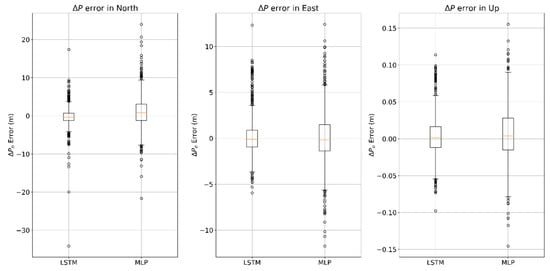
Figure 11. Comparison of multilayer perceptron neural network (MLP) and LSTM algorithms in terms of prediction $\mathsf{\Delta }P$ error.

Table 4. Mean abstract error and standard deviation of $\mathsf{\Delta }P$ in different algorithms. MAE—mean absolute error; LSTM—long short-term memory; MLP—multilayer perceptron neural network.

	LSTM		MLP
$\mathbf{\Delta }\mathit{P}$	MAE	Std	MAE	Std
North (m)	1.573	2.506	3.053	4.109
East (m)	1.422	2.138	1.965	2.686
Height (m)	0.02	0.027	0.027	0.035

The distribution of prediction $\mathsf{\Delta }P$ error in MLP and LSTM algorithms are shown in Figure 11. The value of the mean absolute error (MAE) of the predicting position increments in the north direction using the algorithms of LSTM and MLP are 1.573 m and 3.053 m, respectively, whereas the standard deviation of each algorithm is 2.506 m and 4.109 m, respectively. The value of the mean absolute error of the predicting position increments in the east direction are 1.422 m and 1.965 m, respectively, meanwhile the standard deviations are 2.138 m and 2.686 m, respectively. Table 4 shows that the performance of predicting $\mathsf{\Delta }P$ in LSTM algorithm is more reliable and stable than that in the traditional MLP algorithm.

In order to compare the performance of different models during GNSS outages more specifically, three different length of test path were selected, which were 60 s, 120 s, and 180 s. For dealing with land vehicles, the position, velocity in North and East, as well as heading were selected to display the performances of improving the navigation results during GNSS outages in different algorithms.

5.3.1. 60-s Outage Experiment Results

From Figure 12, Figure 13 and Figure 14 show the navigation results among different algorithms during 60 s GNSS outages. Before 475,330 s, where the GNSS signal is still available, the whole system works on loosely coupled mode, while three algorithms show the same results. When the GNSS signal is assumed outages, and the navigation performance varies in three different methods.

Figure 12. Position errors of 60 s outages with different algorithms.

Figure 13. Velocity errors of 60 s outages with different algorithms.

Figure 14. Heading errors of 60 s outages with different algorithms.

In Figure 12 and Figure 13, the proposed LSTM algorithm obviously outperforms the MLP algorithm and pure INS. The navigation errors of all three methods gradually deteriorates with time during the GNSS signal outages. In Figure 12, the max position error in east of pure INS, MLP, and LSTM is 42.4, 10.7, and 1.5 m; meanwhile, the max position error in north is 15.6, 21.1, and 9.25 m, respectively. In Figure 13 the max velocity error in east of pure INS, MLP, and LSTM is 0.58, 0.95, and 0.12 m/s, meanwhile the velocity error in north is 1.5, 0.24, and 0.32 m/s, respectively. In Figure 14, the heading error among three algorithms is 1.15°, 0.95°, and 0.18°. All the results are summarized in Table 5. At 475,390 s, the system turns to the loosely coupled mode, and navigation error quickly converges both in three methods.

Table 5. Max error of position, velocity, and heading during 60 s GNSS outages in different algorithms.

Max Error	Pure INS		MLP		LSTM
	East	North	East	North	East	North
Position (m)	42.4	15.6	10.7	21.1	1.5	9.25
Velocity (m/s)	0.58	1.5	0.95	0.24	0.12	0.32
Heading (°)	1.15		0.95		0.18

Figure 15 indicates that LSTM can greatly decrease the pure INS’s navigation error. At the end of GNSS outages, the position error of the LSTM algorithm is 80% performance improvement compared with pure INS mode.

Figure 15. 60 s outages trajectory.

5.3.2. 120-s Outage Experiment Results

This section, a longer GNSS signal time and more complicated scene was selected to test the performances of different algorithms. Figure 16, Figure 17 and Figure 18 show the navigation results among different algorithms during 120 s GNSS outages.

Figure 16. Position errors of 120 s outages with different algorithms.

Figure 17. Velocity errors of 120 s outages with different algorithms.

Figure 18. Heading errors of 120 s outages with different algorithms.

From Figure 16, at 474,630 s, the max position error in east of pure INS, MLP, and LSTM is 54.2, 79.7, and 19.4 m, meanwhile the max position error in north is 14.9, 18.6, and 11.3 m. In Figure 17, the max velocity error in east of pure INS, MLP, and LSTM is 1.1, 2.0, and 0.46 m/s, meanwhile the max velocity error in north is 1.1, 0.45, and 0.32 m/s. In Figure 18, the heading error among three algorithms is 0.63°, 0.62°, and 0.27°. All the results are summarized in Table 6.

Table 6. Max error of position, velocity, and heading during 120 s GNSS outages in different algorithms.

Max Error	Pure INS		MLP		LSTM
	East	North	East	North	East	North
Position (m)	54.2	14.9	79.7	18.6	19.4	11.3
Velocity (m/s)	1.1	1.1	2.0	0.45	0.46	0.32
Heading (°)	0.63		0.62		0.27

From Figure 16 and Figure 17, it can be seen that LSTM performs worse in beginning 40 s in north, but for last 80 s, LSTM performs better than MLP for position and velocity in both directions. From the time average performance, LSTM also performs better than MLP.

In Figure 19, under the condition of longer GNSS signal outages and complicated scene with three benches, the performances of all algorithms have reduced, but LSTM also get higher navigation accuracy compared with pure INS. At the end of GNSS outages, the position error of the LSTM algorithm is 68.5% performance improvement compared with the pure INS.

Figure 19. 120 s outages trajectory.

5.3.3. 180-s Outage Experiment Results

This section, a 180 s GNSS signal time was selected to test the performances of different algorithms. Figure 20, Figure 21 and Figure 22 show the navigation results among different algorithms during 180 s GNSS outages.

Figure 20. Position errors of 180 s outages with different algorithms.

Figure 21. Velocity errors of 180 s outages with different algorithms.

Figure 22. Heading errors of 180 s outages with different algorithms.

In Figure 20, the proposed LSTM algorithm is obviously better than the MLP algorithm and pure INS. At 474,500 s, the max position error in east of pure INS, MLP, and LSTM is 460, 280, and 17 m, meanwhile the max position error in north is 303, 115, and 10 m. In Figure 21, the max velocity error in east of pure INS, MLP, and LSTM is 4.6, 3.7, and 0.4 m/s, meanwhile the max velocity error in north is 6.7, 2.8, and 0.7 m/s. In Figure 22, the heading error among three algorithms is 0.7°, 0.75° and 0.55°. All the results are summarized in Table 7.

Table 7. Max error of position, velocity, and heading during 180 s GNSS outages in different algorithms.

Max Error	Pure INS		MLP		LSTM
	East	North	East	North	East	North
Position (m)	460	303	280	115	17	10
Velocity (m/s)	4.6	6.7	3.7	2.8	0.4	0.7
Heading (°)	0.7		0.75		0.55

In Figure 23, under the condition of 180 s GNSS signal outages and complicated scene with three benches, the performances of all algorithms have reduced, but LSTM can also improve the navigation errors. At the end of GNSS outages, the position error of the LSTM algorithm is 95.5% performance improvement compared with the pure INS.

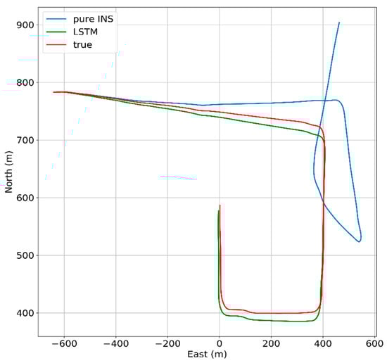
Figure 23. LSTM 180 s outages trajectory.

5.4. Experiment Summary

When the GNSS signal is not available, the whole system turns to predicting mode. The measurements from INS—which are the specific force, velocity, yaw, and angular rate—are sent to a well-trained AI-based model so as to attain a predicting value of position increments. Then, accumulating these position increments can get the pseudo-GNSS position to act as a substitute of the true GNSS position, which will subtract the position measurement from INS to constitute a part of the input vector of the Kalman filter. Finally, the Kalman filter will correct the INS errors so as to attain the corrected position, attitude, and velocity. The test results indicate that the MLP algorithm, which suffers from an incapability of dealing with time-dependency between current and past vehicle dynamics, cannot be a proper model for aiding INS during GNSS signal outages. When the GNSS signal is lost, the LSTM algorithm can get a more accurate navigation result because of its capability of constructing the relationship between future and past information.

6. Conclusions

This paper proposes a novel approach of estimating pseudo measurements employing the LSTM algorithm to reduce the accumulating INS errors when the GNSS signal is blocked. Even in challenging environments, such as complete GNSS outages, this hybrid approach aggregates LSTM neural network, leading to a substantial decrease in position error of vehicle. In this research, the input features and output of the LSTM module were carefully analyzed, where the input features—including the specific force, angular rate, velocity, and yaw—can represent the dynamic vehicle information well. Then, the estimated output was selected as the position increment, which can avoid bringing in additional errors caused by mixing the information of GNSS and INS. Compared with the MLP algorithm, a kind of traditional static neural network, the proposed algorithm based on LSTM can obtain more accurate and stable predictions of navigation results due to its incredible property of dealing with sequential processes. Thus, the LSTM algorithm can provide a more accurate and reliable way to develop a navigation scheme during GNSS outages.

References

- Srinivas, P.; Anil, K. Overview of architecture for GNSS-INS integration. In Proceedings of the 2017 Recent Developments in Control, Automation & Power Engineering (RDCAPE), Noida, India, 26–27 October 2017; pp. 433–438. [Google Scholar]
- Groves, P.D.; Wang, L. The four key challenges of advanced multi-sensor navigation and positioning. In Proceedings of the 2014 IEEE/ION Position, Location and Navigation Symposium—PLANS 2014, Monterey, CA, USA, 5–8 May 2014; pp. 773–792. [Google Scholar]
- Gao, S. Multi-sensor optimal data fusion for INS/GNSS/SAR integrated navigation system. Aerosp. Sci. Technol. 2009, 13, 232–237. [Google Scholar] [CrossRef]
- Li, X.; Chen, W. Multi-sensor fusion methodology for enhanced land vehicle positioning. Inf. Fusion 2019, 46, 51–62. [Google Scholar] [CrossRef]
- Havyarimana, V.; Hanyurwimfura, D. A novel hybrid approach based-SRG model for vehicle position prediction in multi-GNSS outage conditions. Inf. Fusion 2018, 41, 1–8. [Google Scholar] [CrossRef]
- Abdolkarimi, E.S.; Mosavi, M.R. Optimization of the low-cost INS/GNSS navigation system using ANFIS for high speed vehicle application. In Proceedings of the 2015 Signal Processing and Intelligent Systems Conference (SPIS), Tehran, Iran, 16–17 December 2015; pp. 93–98. [Google Scholar]
- Adusumilli, S.; Bhatt, D. A low-cost INS/GNSS integration methodology based on random forest regression. Expert Syst. Appl. 2013, 40, 4653–4659. [Google Scholar] [CrossRef]
- Ye, W.; Liu, Z. Enhanced Kalman Filter using Noisy Input Gaussian Process Regression for Bridging GNSS Outages in a POS. J. Navig. 2018, 71, 565–584. [Google Scholar] [CrossRef]
- Yang, Y.X. Adaptive Navigation and Kinematic Positioning, 2nd ed.; Surveying and Mapping Press: Beijing, China, 2008; pp. 18–19. ISBN 978-7-5030-4005-4. [Google Scholar]
- Du, S.; Gao, Y. Inertial aided cycle slip detection and identification for integrated PPP GNSS and INS. Sensors 2012, 12, 14344–14362. [Google Scholar] [CrossRef]
- Xu, Z. Novel hybrid of LS-SVM and Kalman filter for GNSS/INS integration. J. Navig. 2010, 63, 289–299. [Google Scholar] [CrossRef]
- Sharaf, R.; Noureldin, A. Online INS/GNSS integration with a radial basis function neural network. IEEE Aerosp. Electron. Syst. Mag. 2005, 20, 8–14. [Google Scholar] [CrossRef]
- Sharaf, R.; Noureldin, A. Sensor integration for satellite-based vehicular navigation using neural networks. IEEE Trans. Neural Netw. 2007, 18, 589–594. [Google Scholar] [CrossRef]
- El-Sheimy, N.; Chiang, K.-W.; Noureldin, A. The utilization of artificial neural networks for multisensor system integration in navigation and positioning instruments. IEEE Trans. Instrum. Meas. 2006, 55, 1606–1615. [Google Scholar] [CrossRef]
- Jaradat, M.A.K.; Abdel-Hafez, M.F. Non-linear autoregressive delay-dependent INS/GNSS navigation system using neural networks. IEEE Sens. J. 2017, 17, 1105–1115. [Google Scholar] [CrossRef]
- Li, J.; Song, N. Improving positioning accuracy of vehicular navigation system during GNSS outages utilizing ensemble learning algorithm. Inf. Fusion 2017, 35, 1–10. [Google Scholar] [CrossRef]
- Adusumilli, S.; Bhatt, D. A novel hybrid approach utilizing principal component regression and random forest regression to bridge the period of GNSS outages. Neurocomputing 2015, 166, 185–192. [Google Scholar] [CrossRef]
- Tan, X. GA-SVR and pseudo-position-aided GNSS/INS integration during GNSS outage. J. Navig. 2015, 68, 678–696. [Google Scholar] [CrossRef]
- Indelman, V.; Williams, S.; Kaess, M.; Dellaert, F. Information fusion in navigation systems via factor graph based incremental smoothing. Robot. Auton. Syst. 2013, 61, 721–738. [Google Scholar] [CrossRef]
- Dai, H.F.; Bian, H.W.; Wang, R.Y.; Ma, H. An INS/GNSS integrated navigation in GNSS denied environment using recurrent neural network. Def. Technol. 2019. [Google Scholar] [CrossRef]
- Malleswaran, M.; Vaidehi, V.; Sivasankari, N. A novel approach to the integration of GNSS and INS using recurrent neural networks with evolutionary optimization techniques. Aerosp. Sci. Technol. 2014, 32, 169–179. [Google Scholar] [CrossRef]
- Noureldin, A.; El-Shafie, A.; Bayoumi, M. GNSS/INS integration utilizing dynamic neural networks for vehicular navigation. Inf. Fusion 2011, 12, 48–57. [Google Scholar] [CrossRef]
- Hasan, A.M.; Samsudin, K. GNSS/INS integration based on dynamic ANFIS network. Int. J. Control Autom. 2012, 5, 1–21. [Google Scholar]
- Hochreiter, S.; Jürgen, S. Long short-term memory. Neural Comput. 1997, 9, 1735–1780. [Google Scholar] [CrossRef]
- Wu, Y.; Schuster, M.; Chen, Z. Google’s neural machine translation system: Bridging the gap between human and machine translation. arXiv 2016, arXiv:1609.08144. [Google Scholar]
- Ma, X. Long short-term memory neural network for traffic speed prediction using remote microwave sensor data. Transp. Res. Part C Emerg. Technol. 2015, 54, 187–197. [Google Scholar] [CrossRef]
- Duan, Y.; Lv, Y.; Wang, F.Y. Travel time prediction with LSTM neural network. In Proceedings of the 2016 IEEE 19th International Conference on Intelligent Transportation Systems (ITSC), Rio de Janeiro, Brazil, 1–4 November 2016; pp. 1053–1058. [Google Scholar]
- Zhang, Y. Hybrid algorithm based on MDF-CKF and RF for GNSS/INS system during GNSS outages. IEEE Access 2018, 6, 35343–35354. [Google Scholar] [CrossRef]
- Trawny, N.; Mourikis, A.I. Vision-aided inertial navigation for pin-point landing using observations of mapped landmarks. J. Field Robot. 2007, 24, 357–378. [Google Scholar] [CrossRef]
- Groves, P.D. Principles of GNSS, Inertial, and Multisensor Integrated Navigation Systems; Artech House: London, UK, 2013. [Google Scholar]
- Julier, S.J.; Uhlmann, J.K. New extension of the Kalman filter to nonlinear systems. Aerosense Int. Soc. Opt. Photonics 1997. [Google Scholar] [CrossRef]
- Fernando, T. Soft hardwired attention: An lstm framework for human trajectory prediction and abnormal event detection. Neural Netw. 2018, 108, 466–478. [Google Scholar] [CrossRef]
- Zhao, Z.; Chen, W. LSTM network: A deep learning approach for short-term traffic forecast. IET Intell. Transp. Syst. 2017, 11, 68–75. [Google Scholar] [CrossRef]
- Saleh, K.; Mohammed, H.; Saied, N. Intent prediction of vulnerable road users from motion trajectories using stacked LSTM network. In Proceedings of the 2017 IEEE 20th International Conference on Intelligent Transportation Systems (ITSC), Yokohama, Japan, 16–19 October 2017. [Google Scholar]
- Xingjian, S.H.I. Convolutional LSTM network: A machine learning approach for precipitation nowcasting. Adv. Neural Inf. Process. Syst. 2015, 28, 802–810. [Google Scholar]
- Bhatt, D. A novel hybrid fusion algorithm to bridge the period of GNSS outages using low-cost INS. Expert Syst. Appl. 2014, 41, 2166–2173. [Google Scholar] [CrossRef]
- Abdel-Hamid, W.; Noureldin, A. Adaptive fuzzy prediction of low-cost inertial-based positioning errors. IEEE Trans. Fuzzy Syst. 2007, 15, 519–529. [Google Scholar] [CrossRef]
- Farrell, J.; Barth, M. The Global Positioning System and Inertial Navigation; Mcgraw-Hill: New York, NY, USA, 1999; Volume 61. [Google Scholar]
- Goshen-Meskin, D.; Bar-Itzhack, I.Y. Unified approach to inertial navigation system error modeling. J. Guid. Control Dyn. 1992, 15, 648–653. [Google Scholar]
- Liu, W.; Wen, Y. Large-margin softmax loss for convolutional neural networks. In Proceedings of the 33rd International Conference on Machine Learning, New York, NY, USA, 19–24 June 2016; pp. 507–516. [Google Scholar]
- Abadi, M.; Paul, B. Tensorflow: A system for large-scale machine learning. In Proceedings of the OSDI’16: 12th USENIX conference on Operating Systems Design and Implementation, Savannah, GA, USA, 2–4 November 2016; pp. 265–283. [Google Scholar]
- Diederik, K.; Jimmy, B. Adam: A method for stochastic optimization. In Proceedings of the 3rd International Conference for Learning Representations, San Diego, CA, USA, 7–9 May 2015. [Google Scholar]
© 2020 by the authors. Licensee MDPI, Basel, Switzerland. This article is an open access article distributed under the terms and conditions of the Creative Commons Attribution (CC BY) license (http://creativecommons.org/licenses/by/4.0/).