Article

Understanding Inter-Hemispheric Traveling Ionospheric Disturbances and Their Mechanisms
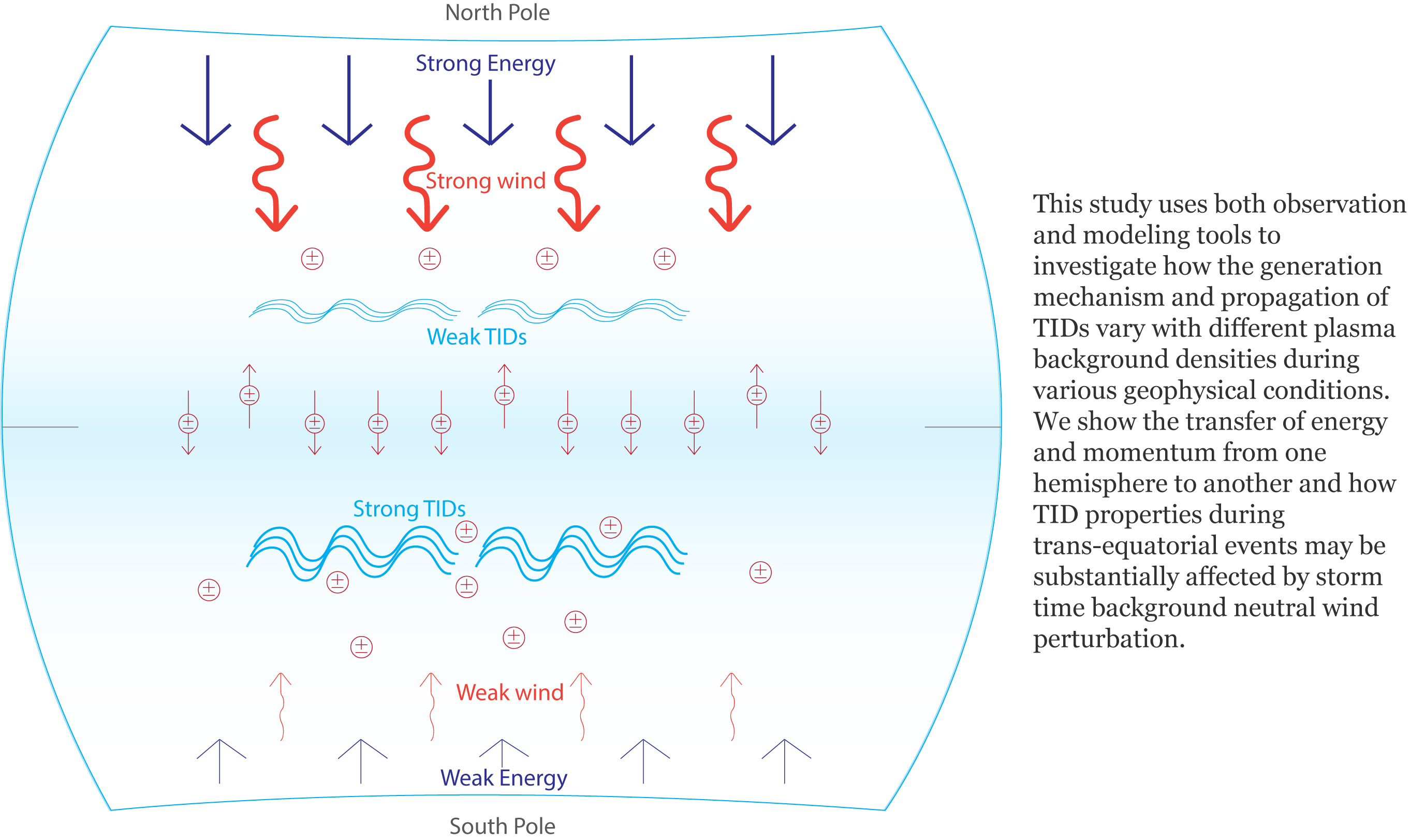
by
Olusegun F. Jonah
1,*,
Shunrong Zhang
1,
Anthea J. Coster
1,
Larisa P. Goncharenko
1,
Philip J. Erickson
1,
William Rideout
1,
Eurico R. de Paula
2 and
Rodolfo de Jesus
2
1
Haystack Observatory, Massachusetts Institute of Technology, 99 Millstone Rd, Westford, MA 01886, USA
2
National Institute for Space Research (INPE), Sao Jose dos Campos, SP 12227-010, Brazil
*
Author to whom correspondence should be addressed.
Remote Sens. 2020, 12(2), 228; https://doi.org/10.3390/rs12020228
Submission received: 18 November 2019 / Revised: 27 December 2019 / Accepted: 3 January 2020 / Published: 9 January 2020
(This article belongs to the Special Issue Remote Sensing of Ionosphere Observation and Investigation)

Abstract

:
Traveling ionospheric disturbances (TIDs) are wave-like disturbances in ionospheric plasma density. They are often observed during both quiet (medium-scale TID) and geomagnetically disturbed (large-scale TID) conditions. Their amplitudes can reach double-digit percentages of the background plasma density, and their existence presents a challenge for accurate ionosphere specification. In this study, we examine TID properties using observations obtained during two geomagnetically disturbed periods using multiple ground and space-borne instruments, such as magnetometers, Global Navigation Satellite System (GNSS) receivers, and the SWARM satellite. Reference quiet time observations are also provided for both storms. We use a thermosphere–ionosphere–electrodynamics general circulation model (TIEGCM) results to properly interpret TID features and their drivers. This combination of observations and modeling allows the investigation of variations of TID generation mechanisms and subsequent wave propagation, particularly as a function of different plasma background densities during various geophysical conditions. The trans-equatorial coupling of TIDs in the northern and southern hemispheres is also investigated with respect to attenuation and propagation characteristics. We show that TID properties during trans-equatorial events may be substantially affected by storm time background neutral wind perturbation.

Graphical Abstract

1. Background Introduction

Over the decades, since the initial work by Hines [1], a large variety of traveling ionospheric disturbances (TIDs) have been observed in the upper atmosphere. These TIDs are wavelike structures in the ionospheric density and can be classified into two groups according to basic characteristics [2]: medium-scale TIDs (MSTIDs) and large-scale TIDs (LSTIDs). MSTIDs are wavelike disturbances in ionospheric electron density with typical characteristics of 50–250 m/s horizontal velocities, 100–500 km, horizontal wavelengths with a distribution peak at 250 km, and 15 to 60-min periods [3,4]. These parameters suggest that MSTIDs may be associated with thermospheric gravity waves [5] and therefore may ultimately have various meteorological sources, including tropospheric events [3,6,7]. MSTIDs are present during both day and night, and their configurations and direction of propagation depend mainly on the source location and the associated electrodynamic properties of the ionospheric medium [8].
On the other hand, large-scale traveling ionospheric disturbances (LSTIDs) propagate signatures of energy transfer throughout the ionospheric system mainly during geomagnetic storms, and thus serve as a strong indicator of magnetosphere/ionosphere/thermosphere coupling. LSTIDs are typically generated by auroral sources at high latitudes [2,9], although some have been observed to be associated with the solar terminator [10]. LSTIDs can have significant amplitudes, up to 20% of the background total electron content (TEC), with 500–1000 m/s horizontal velocities, 1000–3000 km wavelengths, and 60 min to 2+-h wave periods [11,12]. Recent studies have shown different propagation speeds of LSTIDs at different longitudes [6,13], and one researcher developed a method for determining the characteristics of LSTID’s parameters based on calculations of the spatial and temporal gradients of TEC as measured at three distributed GPS receivers. He found that LSTIDs excited in the auroral region traveled equatorward to a distance of more than 2000 km with a velocity of 300 m/s and a front width of 3700 km. Other types of TIDs have been associated with ionospheric irregularities [14]. For example, Kil and Paxton [14] investigated the role of MSTIDs in the creation of electron density irregularities in the middle latitudes using SWARM observations and concluded that MSTIDs can emerge as a source of irregularities during solstice season.
Ionospheric disturbances such as TIDs have been detected by many instruments, such as incoherent scatter radars, high-frequency (HF) Doppler sounders, ionosondes, radio telescopes [15], and airglow imagers [16]. An important technique for measuring TIDs is GNSS-TEC. The experimental GNSS-TEC technique is employed in this study due to its relatively wide spatial coverage as compared to other instruments. Data from observational system and theoretical studies have been used both separately and jointly to investigate the sources and mechanisms responsible for TIDs e.g., [1,3,6,7,11,17,18,19,20].
Other studies have provided information on the preconditioning influence of background neutral atmospheric conditions on TID features. In particular, Cowling et al. [21] and Waldock and Jones [22] examined the effect of background winds on the trajectory of a wave-packet of an internal gravity wave by using ray-tracing in a wind-stratified model atmosphere. They found that wind acts as a directional filter, in that only waves propagating in certain directions are able to travel significant distances.
Since thermospheric wind may affect the propagation of internal waves in a profound way, wind oscillations can also influence acoustic gravity waves and traveling ionospheric disturbances effects in the F-region heights. Multiple studies support this conclusion and furthermore show that the effects are multi-faceted. Storm time thermospheric perturbations can be particularly significant: using the incoherent scatter radar (ISR) technique to measure thermospheric wind, Vasseur [23] showed that wind speed under disturbance conditions can reach amplitudes as large as 200 m/s. This value may exceed the horizontal phase velocity of acoustic waves, and the propagation of such waves in the atmosphere (especially those with a lower phase speed) is correspondingly expected to be influenced to a large degree by thermospheric winds [21]. Based on the characteristics of TIDs described in present study, these TIDs waves can be mostly associated with gravity waves.
Furthermore, neutral wind perturbations, as part of traveling atmospheric disturbances (TADs) [24,25] originated at high latitudes during storms, can significantly alter the stormtime thermospheric general circulation and plasma dynamics. The ions are set in motion both parallel and perpendicular to the geomagnetic field. The parallel ion drift oscillates due to the oscillation of the neutral wind field-aligned component, which drags the ions through ion-neutral collisions, causing large scale TIDs. The perpendicular ion drift is associated with zonal electric fields established by various electrodynamic processes, including the disturbance wind dynamo [26], which produces polarization electric fields during the equatorward propagation of disturbance winds. Habarulema et al. [15] noticed that storm-induced equatorward winds during solstice conditions travel in the same direction as background neutral winds blowing from the summer to the winter hemisphere, driving the production of equatorward TIDs in the region. They also suggested that the meridional wind component of the neutral wind plays a significant role in the poleward TID propagation direction in the northern hemisphere. However, the range of important processes in general remains relatively poorly understood.
These complex and interlocked TID generation and propagation mechanisms, and others not yet discovered, introduce significant variability to the ionosphere and thermosphere (IT) system and remain insufficiently understood and quantified. In particular, the identification of important TID sources has not yet been comprehensively accomplished, and the mechanisms by which they are coupled to different atmospheric regions are not yet fully understood. These tasks are important to not only establish a baseline understanding of their intrinsic characteristics, but also to quantitatively understand their contribution to atmospheric variability. This makes the understanding of TID sources and propagation mechanisms important for advancing an understanding of the whole atmosphere dynamic response. The present study aims to enlighten our understanding on the aforementioned problems and contributes to the interpretations of TID dynamics by providing insight into cross-equatorial TID propagation, characteristics, and mechanisms. In Section 2, we present the material and method used for both observation and simulation. Section 3 presents the results based on two geomagnetic storms, and in Section 4, we discussed the mechanisms for the different behavior of cross-equatorial TIDs observed.

2. Materials and Methods

The total electron content data used in this study were collected from the Madrigal website at http://millstonehill.haystack.mit.edu/. All available TEC data between about 30° N and 30° S latitudes and 55° W and 75° W longitudes, as shown in Figure 1a, were employed in this investigation. The blue dots represent the ionospheric pierce point distribution of the TEC measurement on 8 May 2017 at 10:00 UT, and the black line represents the magnetic equator.
The line of sight TEC (STEC) was converted to vertical TEC (VTEC) at the pierce point of 300 km altitude. The GNSS-TEC processing algorithms used at Haystack were originally developed by Rideout and Coster [27] and updated by Vierinen et al [28]. To obtain the signature of TIDs from TEC data, background TEC data were filtered by using a technique similar to that of Coster et al. [17] and Zhang et al. [20]. More extended discussion of this TID detection technique was given in Zhang et al. [29]. Figure 1b represents differential TEC (∆TEC) analysis procedures, with 1 TEC = 1016el/m2. The blue line represents the background TEC from one station and two PRN (PRN are the pseudo-random noise codes that each satellite transmits), the red line represents the hourly sliding window using the Savitzky–Golay low-pass filter, and the black line represents the ∆TEC. This process includes a convolution method with least squares fitting of simultaneous subsets of 60 min length involving adjacent VTEC data points obtained from GNSS satellite–receiver pairs. Using this method, the error in differential TEC is determined by the phase noise of the receivers. This error is typically 0.01 TECu (1 TECu = 1016 electron/m2), which is significantly less than the magnitude of a typical TID.

2.1. Magnetometer and Geophysical Data

We also used magnetometer data collected from three different networks: SuperMAG, Amber, and LISN. In total, six magnetometer stations were used. T51 (48.05N, 77.78W) and AIA (65.3S, 65.3W) were downloaded from the SuperMAG network, Belem (1.45S, 48.5W) and Petrolina (9.5S, 40.5W) were downloaded from the Amber network, and Jicamarca (11.95S, 76.88W) and Piura (5.2S, 80.6W) were downloaded from the LIST network. The T51 and AIA stations are located around the Auroral region, while the Belem, Piura, Petrolina and Jicamarca stations are located around and off the equator, respectively.
Solar wind (Vsw) data were obtained from the ACE satellite mission: https://www.swpc.noaa.gov/products-and-data. Interplanetary magnetic field (Bz), auroral electrojet (AE), symmetric magnetic field strength (Sym-H), interplanetary electric field (Ey), and Kp indices were obtained from the NASA database network at http://omniweb.gsfc.nasa.gov.

2.2. TIE-GCM Model

The thermosphere–ionosphere–electrodynamics general circulation model (TIE-GCM) [30] is a comprehensive, first-principle, three-dimensional, non-linear representation of the coupled thermosphere and ionosphere that includes a self-consistent solution of the low-latitude electric field. It comprises the physical and chemical processes relevant for the upper stratosphere and self-consistently solves the Eulerian continuity, momentum, and energy equations involving the coupled ionosphere and thermosphere system. The model is built on a spherical coordinate system fixed relative to the rotating Earth with horizontal latitude and longitude axes and a vertical pressure surfaces axis. The model computes global distributions of the neutral gas temperature and winds, the height of the constant pressure surface, and the number densities of major constituents, i.e., O2, N2, and O, including certain minor neutral constituents. TIE-GCM includes boundaries of approximately 97 km and 500 km and a resolution of 5° × 5° in latitude and longitude, and the model results provide important information on both the thermospheric and ionospheric dynamics that is useful when discussing potential mechanisms for variations directly observed in TEC.
TIE-GCM simulations for two selected storm intervals were conducted online as provided by the Community Coordinated Modeling Center (CCMC). To determine the high-latitude electric field, we used the option of the Heelis convection model. Other input detail included day 148 (May, 28) of 2017, realistic Kp changing from 4- to 7+ as in the observation, period-measured solar wind speed varying from 300 km/s to 400 km/s in accordance with observations, and interplanetary magnetic field (Bz 20 nT peak) matching observations. This study presents results for a longitude of 65° W, latitude of ±60°, and altitude of 300 km, over a time period of 08:00–23:00 UT.

3. Results

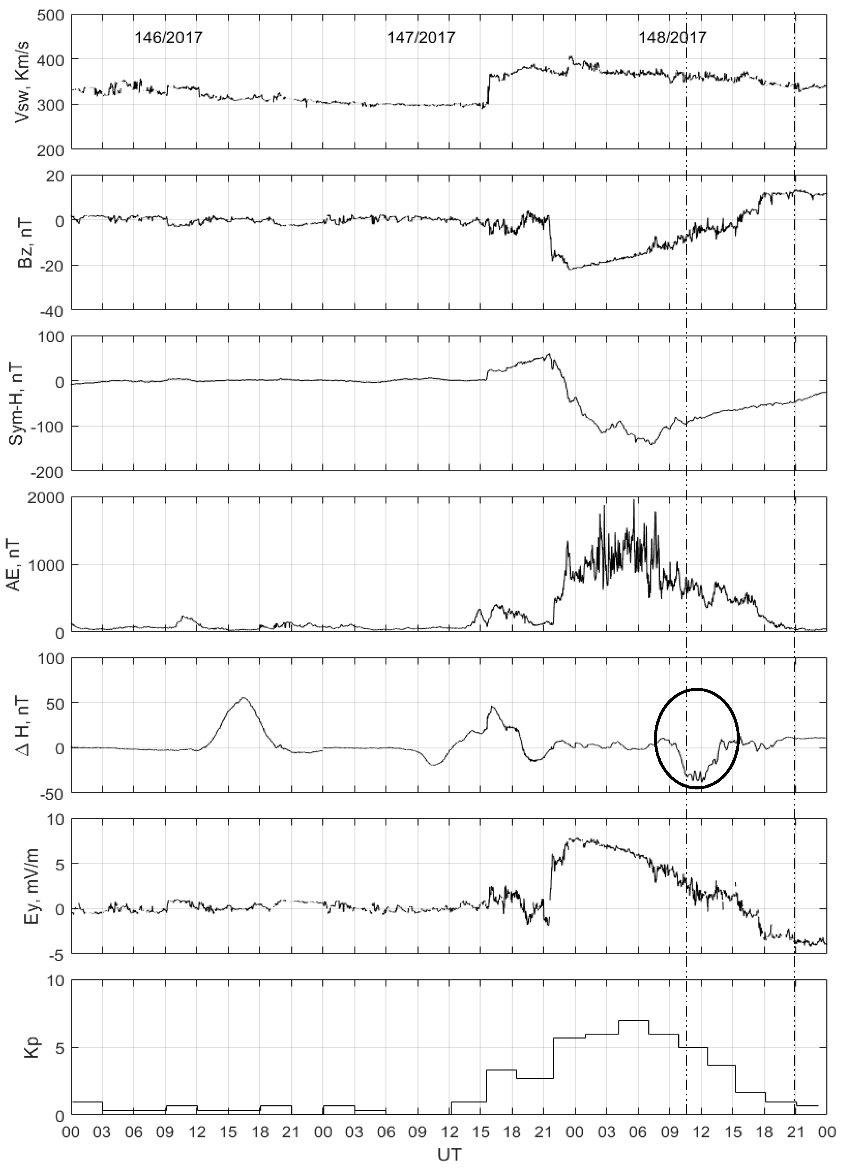
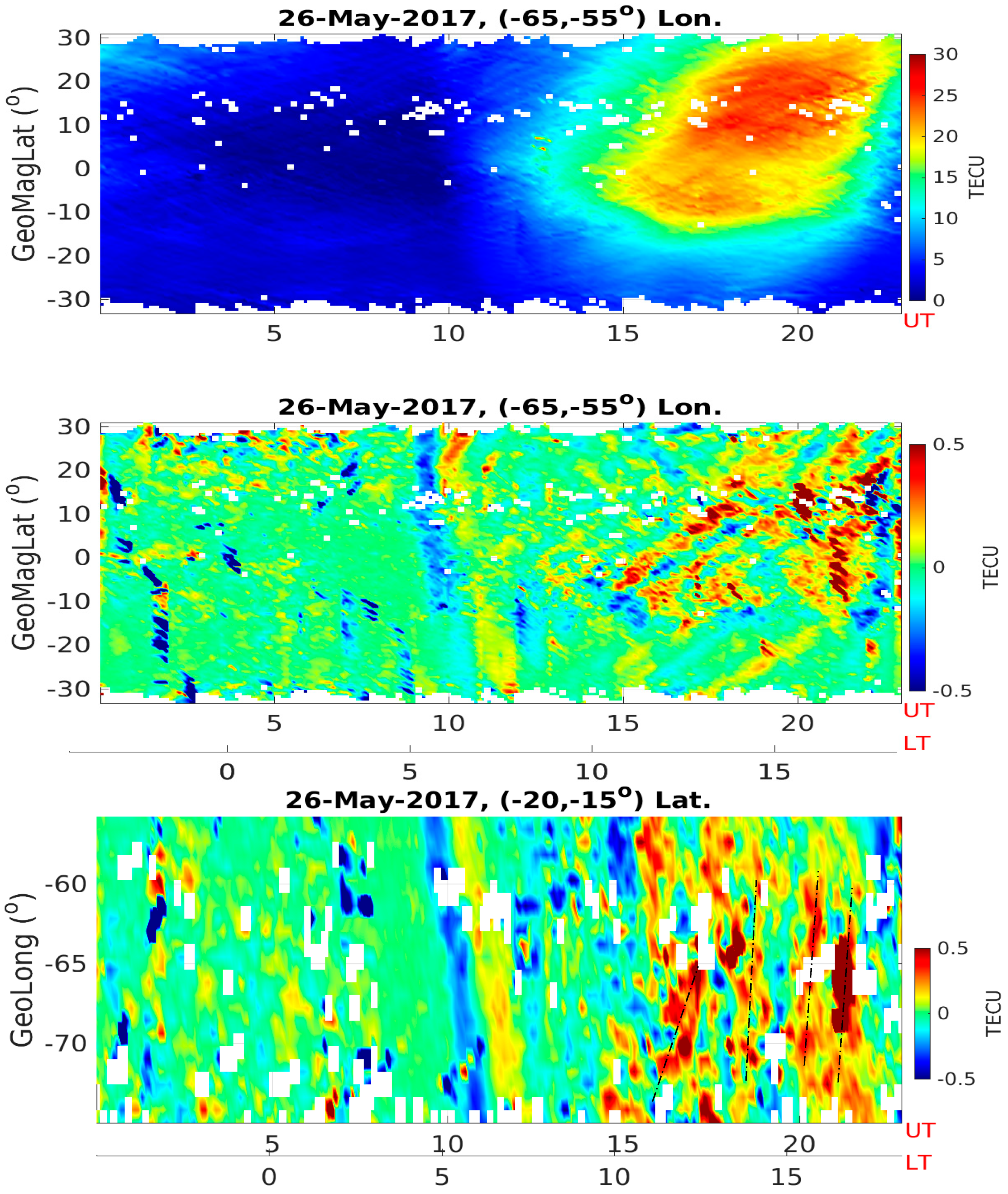
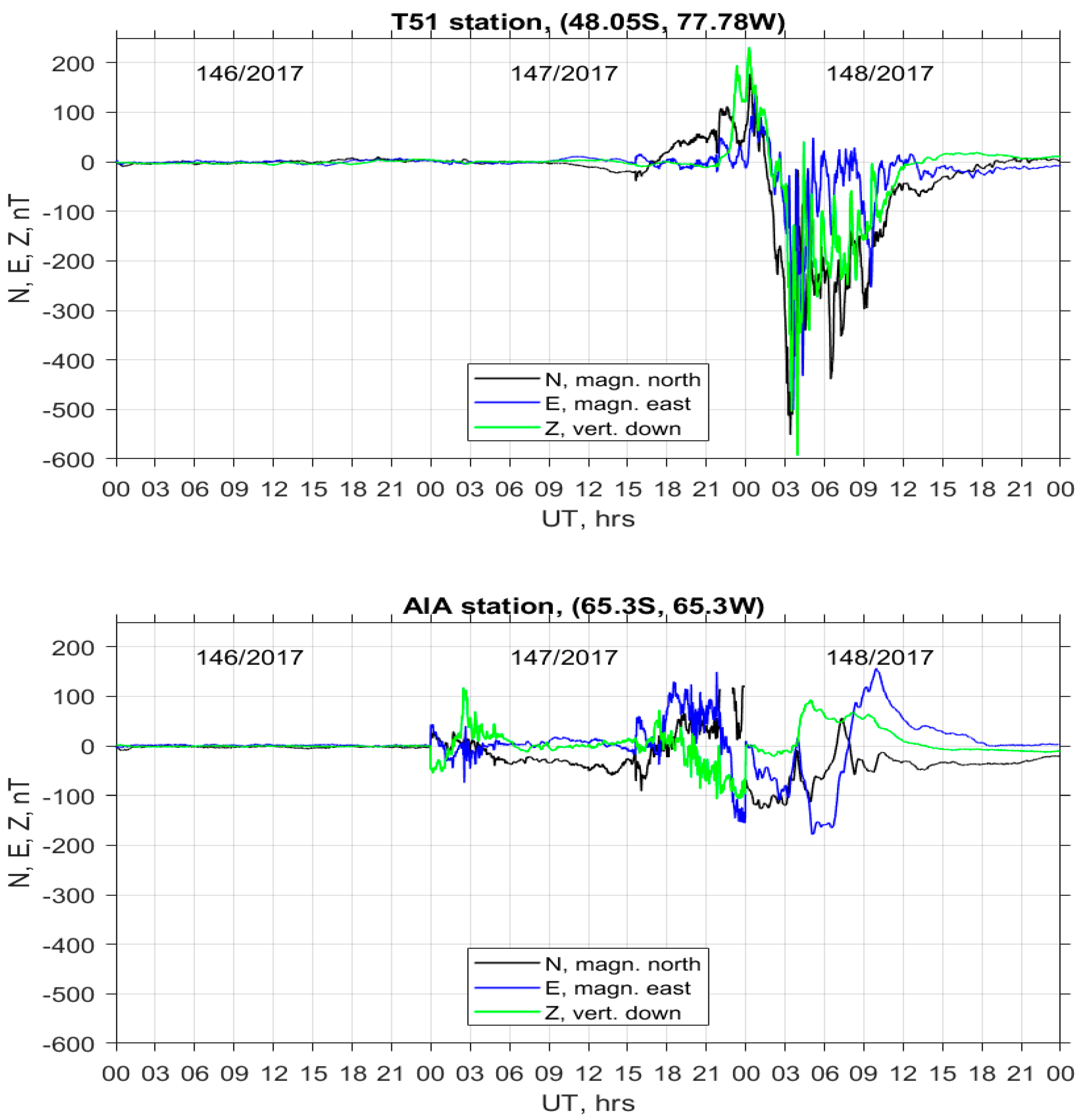
3.1. 2017 Memorial Day Weekend Geomagnetic Disturbance

Figure 2 shows the geophysical and geomagnetic conditions during the first storm interval on 26–28 May 2017. From top to bottom: solar wind speed (Vsw) abruptly increased after approximately 15 UT on 27 May 2017; the Bz component of the magnetic field of the interplanetary magnetic field (IMF) went down to −20 nT for more than three hours; the Sym-H index reached a pronounced minimum of −120 nT, which indicates an intense storm; the AE index increased suddenly from approximately 200 to 1500 nT; ∆H (Belem–Petrolina) behaved normally on days 26 and 27, but turned downward on day 28 opposite to the observed trend in plasma density and TEC. There was a sudden increase in the interplanetary east–west electric field, Ey (positive to east) at the time of Bz southward turning; and the Kp magnetic index was close to 8. The dashed lines highlight the time periods when different features of TIDs were observed.

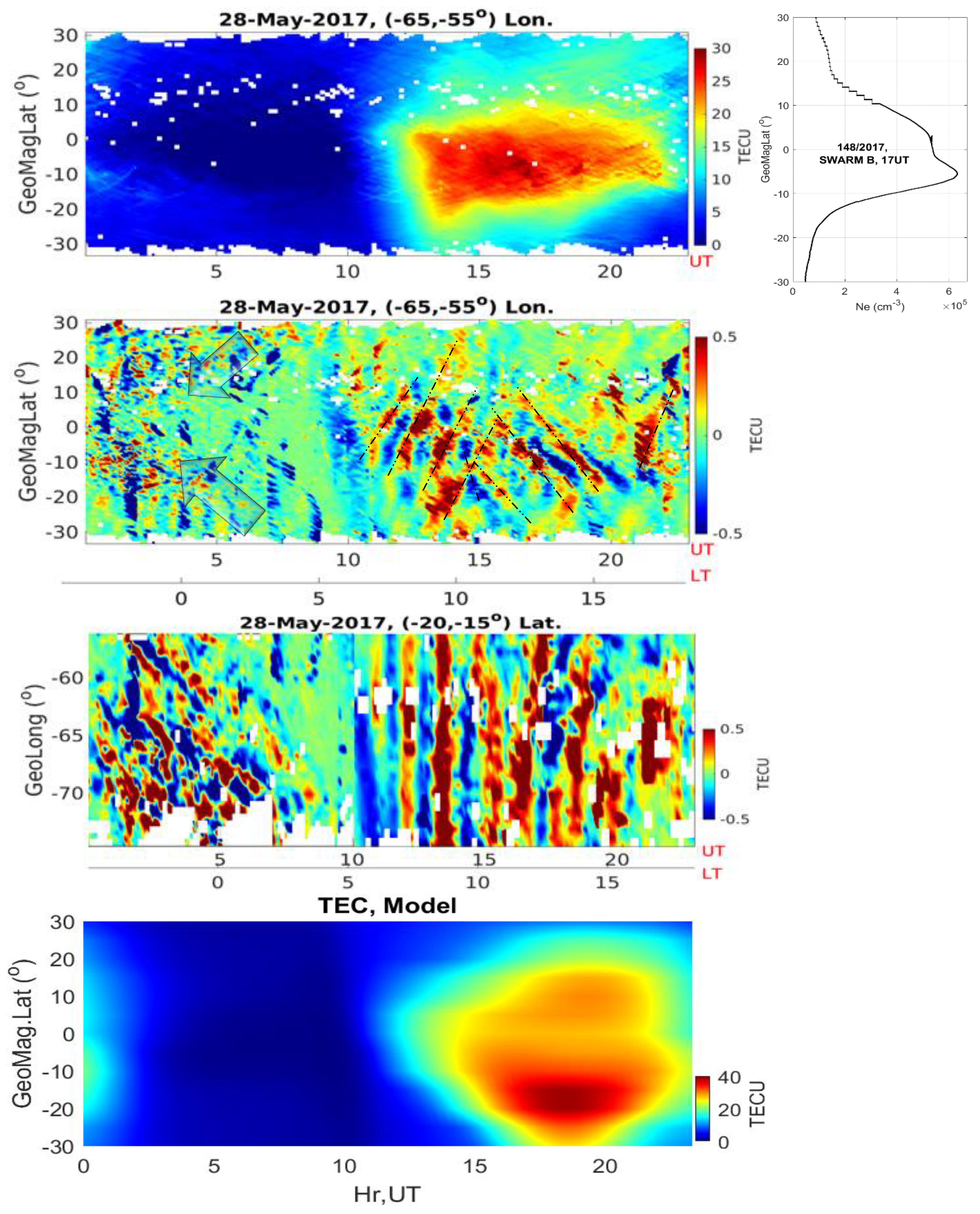
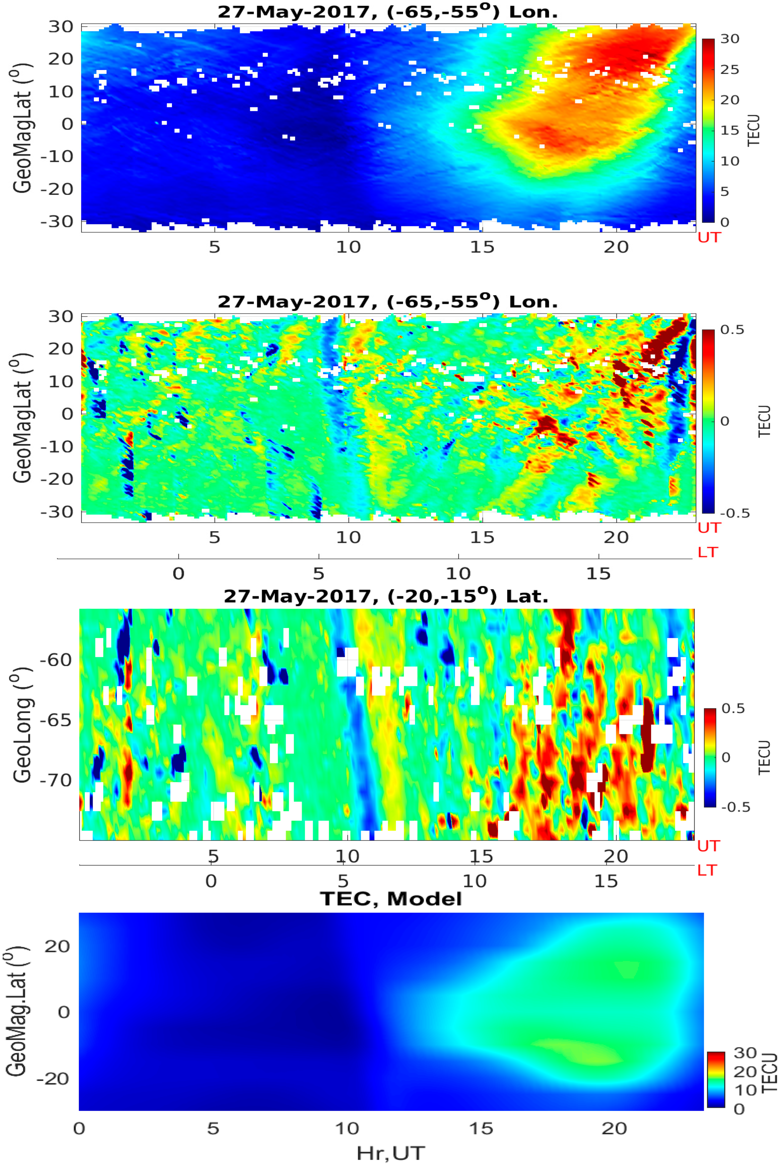
3.2. Interhemispheric TID Coupling Investigation, May 2017

Figure 3 shows the ionospheric response during the May 2017 storm. The top panel plots a keogram of the background total electron content (TECo) with in situ topside electron density (Ne) from the SWARM B satellite on the right-hand side. The data for the keogram were obtained from 65–55° W longitudes and 45° S to 25° N latitudes (geomagnetic latitudes of ±30°). An enhancement in the background TECo of about 35 TECU occurred from around 12:00 UT to 21:00 UT during the recovery phase of the geomagnetic storm at the equatorial and southern region, compared to less than 10 TECU observed over the northern region during the same period. This observation is counter to what would be expected from normal quiet-time solar irradiation at low latitudes. In particular, for the study period, the northern hemisphere (NH) is the summer hemisphere, the southern hemisphere (SH) is the winter hemisphere, and a larger photoionization rate is expected due to smaller solar zenith angle in the NH compared to the SH.
The second panel of Figure 3 plots the latitude keogram of the detrended TEC from (−65, 55) degrees longitude, providing information on meridional TID propagation and behavior during the daytime and nighttime. For nighttime, between 0:00 and 5:00 UT, during the main phase of the geomagnetic storm, weak MSTIDs occurred symmetrically and were mirrored in the opposite hemisphere, although their amplitude is small and relatively difficult to see. However, during the daytime period, between 10:00 and 22:00 UT in the storm recovery phase, we observed well-defined TIDs that were stronger in the SH than in the NH. These wave structures propagated from SH to NH between 10:00 UT and 15:30 UT, and then turned southward at 16:00 UT until 21:00 UT, with a different velocity. The northward TIDs propagated faster with a velocity of 280 ± 12 m/s, while the southward ones propagated with a velocity of 150 ± 10 m/s. The TIDs were more noticeable in the magnetic southern region and appeared to experience attenuation near the equator (approximately 5N geomagnetic) as they moved northward. Overall, the daytime TIDs appear to be more prominent in the SH than in the NH. In Section 4, we show using TIEGCM simulation that TID properties during these transequatorial events are associated with the presence of storm-time background neutral wind perturbations arising from joule heating and auroral precipitation-induced disturbances as well as changes in the O/N2 ratio composition across hemispheres.
The third panel of Figure 3 plots longitude keograms of detrended TEC from (−20, −15) degree latitudes, providing information on east–west TID propagation. The results indicate that strong westward TID propagation occurred during the nighttime at around 0:00–5:00 UT, with a velocity of 102 + 8 m/s and strong TIDs propagated in the eastward direction at around approximately 15:00–23:00 UT with a faster velocity of 514 + 20 m/s. The fourth panel shows TIEGCM simulation results for TEC background conditions on the geomagnetically disturbed day. These model results demonstrate a well-reproduced TEC asymmetry with larger TEC in the SH.
Figure 4 and Figure 5 provide observations on two quiet (non-storm) days for comparison to the storm conditions of Figure 3, using the same geographic regions to construct longitude and latitude keograms for TID detection. Quiet conditions are plotted for 27 May 2017 (Figure 4) and 26 May 2017 (Figure 5). For background TEC (top panel), both Figure 4 and Figure 5 show higher values in the NH at around 15:00–23:00 UT, contrary to the storm time background TEC in Figure 3. For both quiet days, TIDs are observed mostly in the NH around 15:00–23:00 UT (where background density is higher) propagating in the northward direction, similar to the storm-day observation in Figure 3 on 28 May 2017. However, at nighttime (0:00–5:00 UT), clear TIDs were not observed on quiet days, in sharp contrast to multiple nighttime TIDs observed at 0:00–5:00 UT during the storm main phase on 28 May 2017 (Figure 3). The bottom panel’s longitude keogram indicates that on both quiet days (Figure 4 and Figure 5), mostly eastward TID propagation occurred during the daytime, but no westward TID propagation occurred during the nighttime. Figure 4 (bottom panel) shows an example of TIEGCM simulation during quiet conditions, which is similar to observation results at the top of the figure.
Finally, we note that all the TID longitude and latitude keograms in Figure 3, Figure 4 and Figure 5 have an artificial boundary at 10:00 UT related to the quick change from negative to positive in electron density around the normal passage of the sunrise terminator.

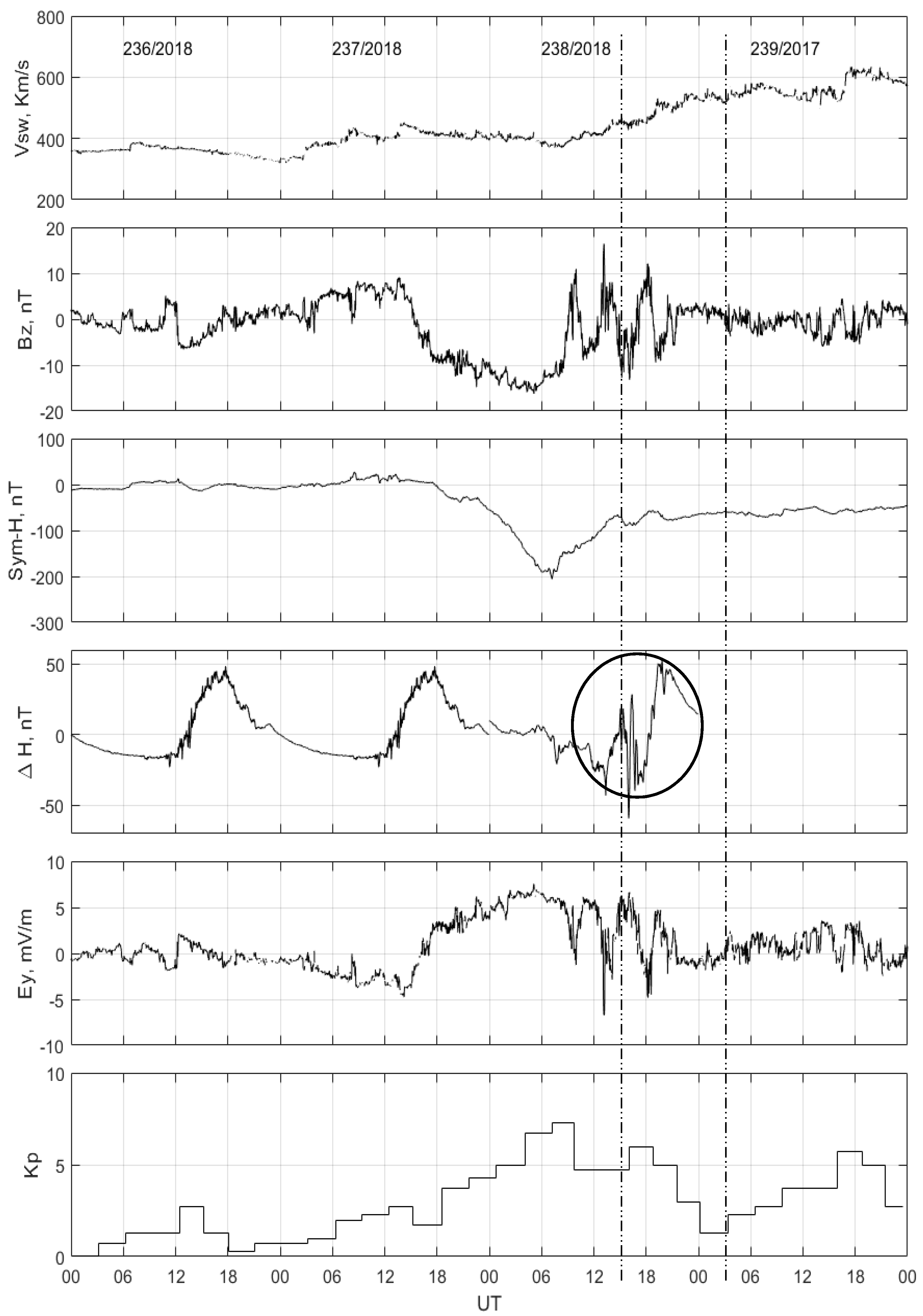
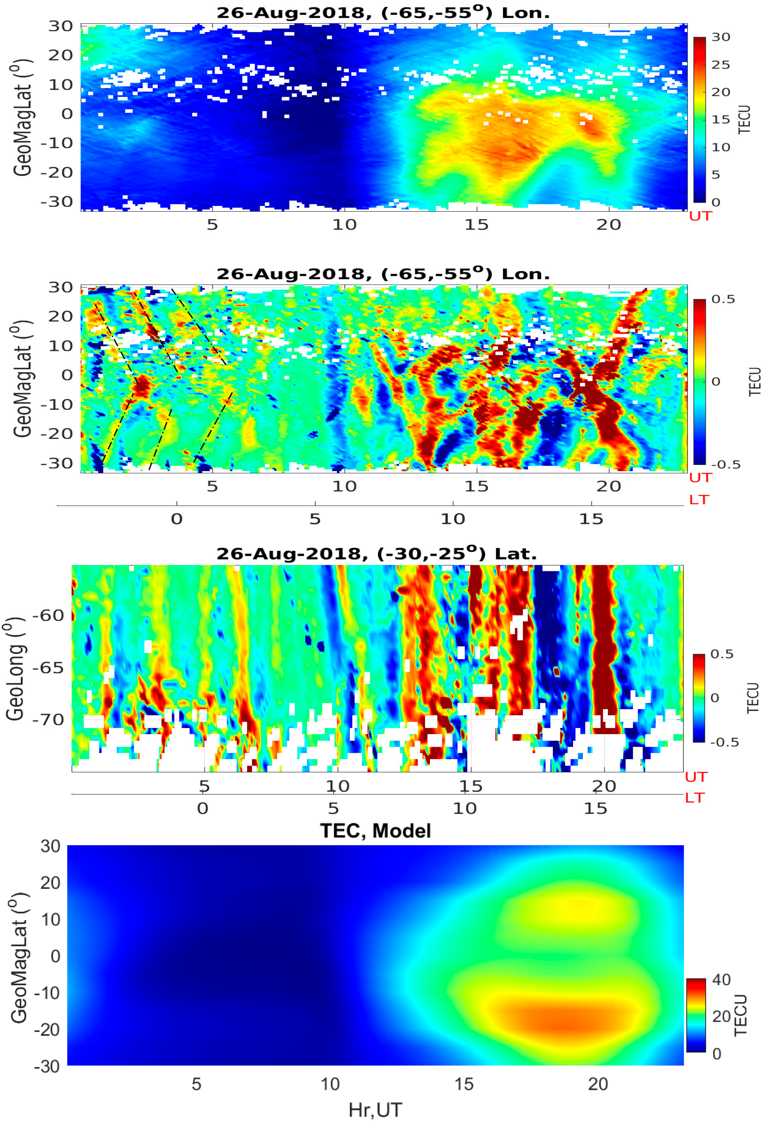
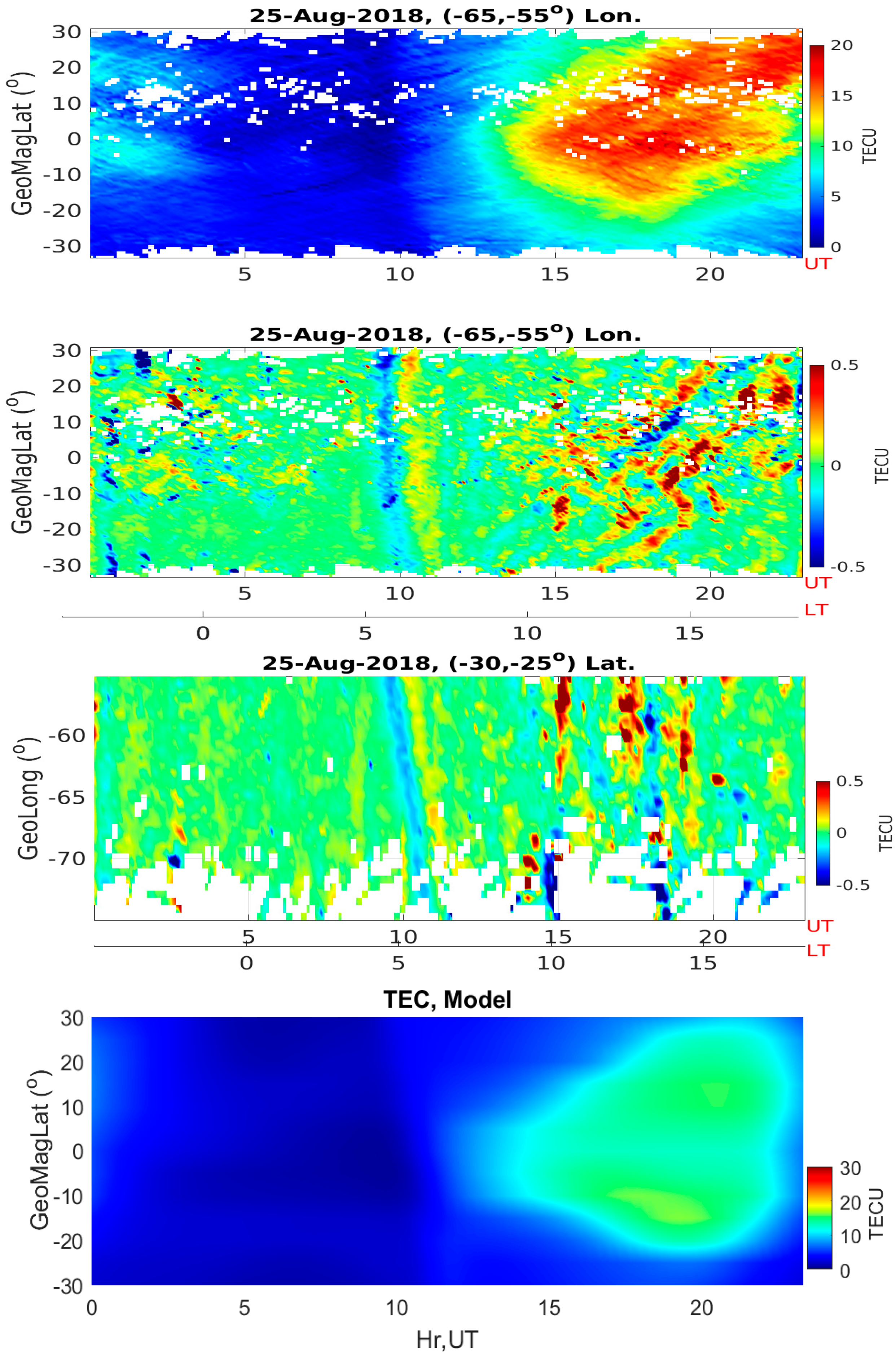
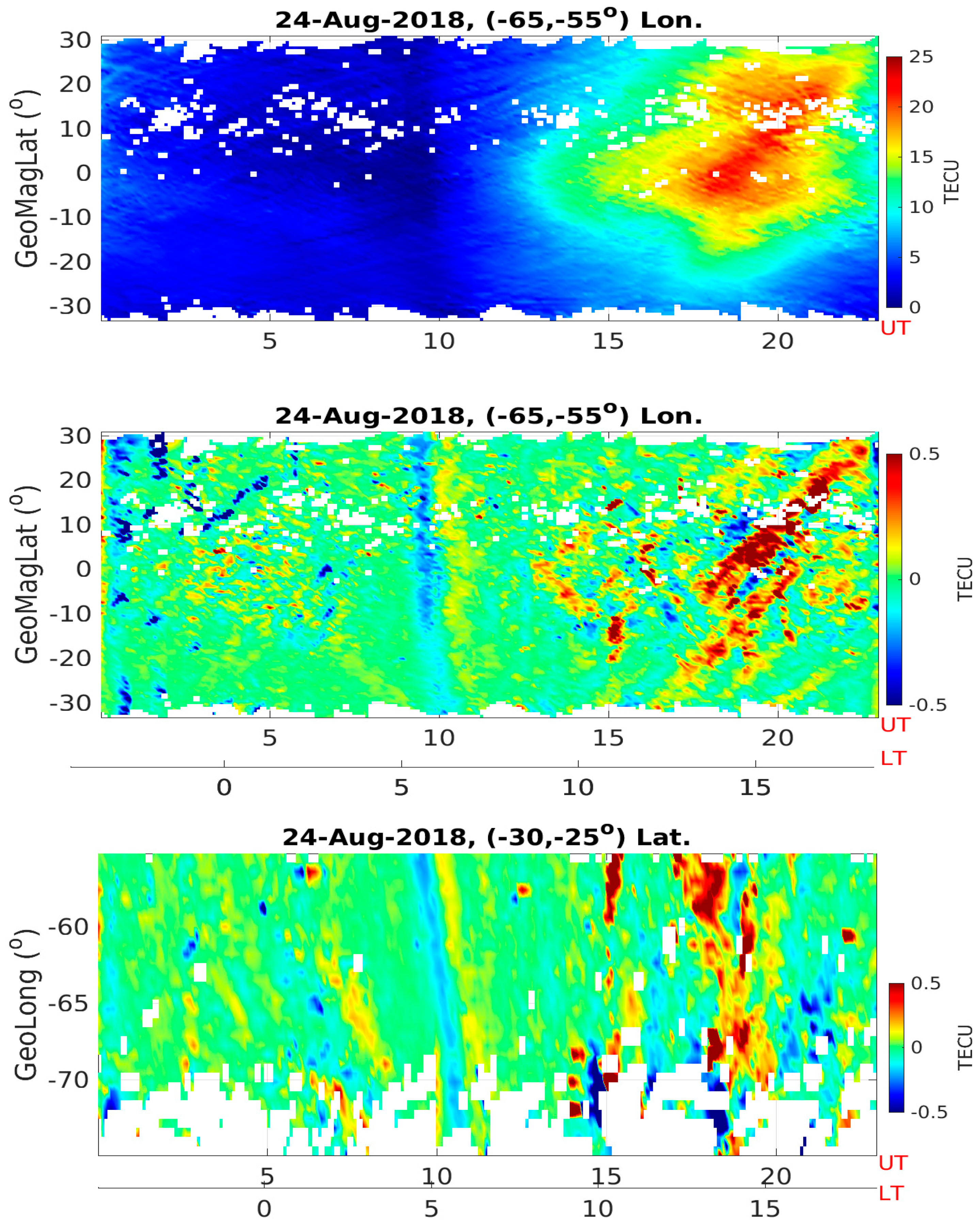
3.3. August 2018 Geomagnetic Storm

To discern whether the 27 May 2017 storm was a unique event in its behavior, we investigate a second storm on 26 August 2018. Figure 6 shows the three days of geophysical and geomagnetic conditions from 24–27 August 2018. From top to bottom, the panels show a gradual increase in the solar wind (Vsw), which is a strong oscillation of Bz from north to south during a long period. The northward surge of Bz during each oscillation is likely to have triggered a prompt penetration electric field [31,32], which gave rise to an observed counter-electrojet (as seen in ∆H) during the same period of Bz anomaly behavior. Sym-H shows that the geomagnetic was very intense. ∆H (Jicamarca–Piura) behaved normally on storm days 24 and 25 but turned downward on day 26 with some intermittent oscillations, similar to the 28 May 2017 storm (cf. Figure 2). Solar wind Bz oscillations were also observed in Ey with similar magnitude. The Kp for this August storm went up to 7+ units. AE data was not available on all three days. The dashed lines represent the time periods when different features of TIDs were observed.

3.4. Interhemispheric TID Coupling Investigation, August 2018
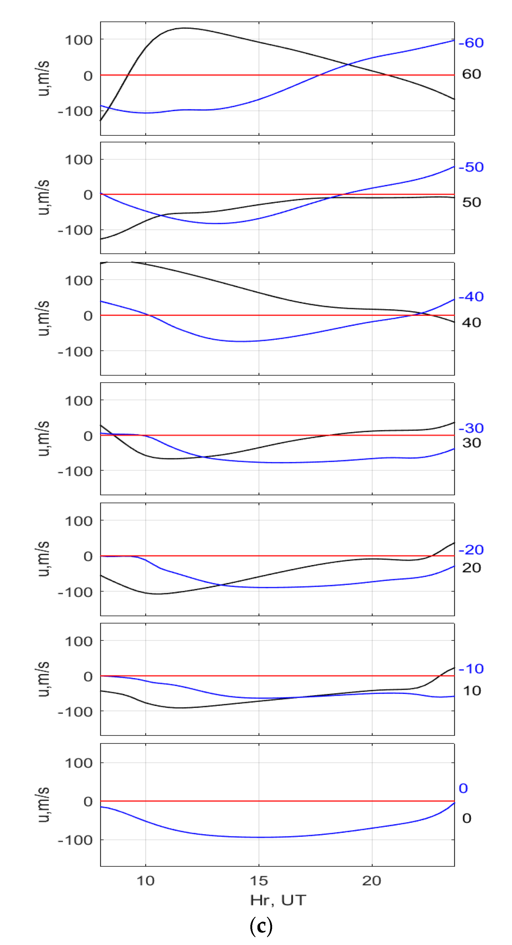
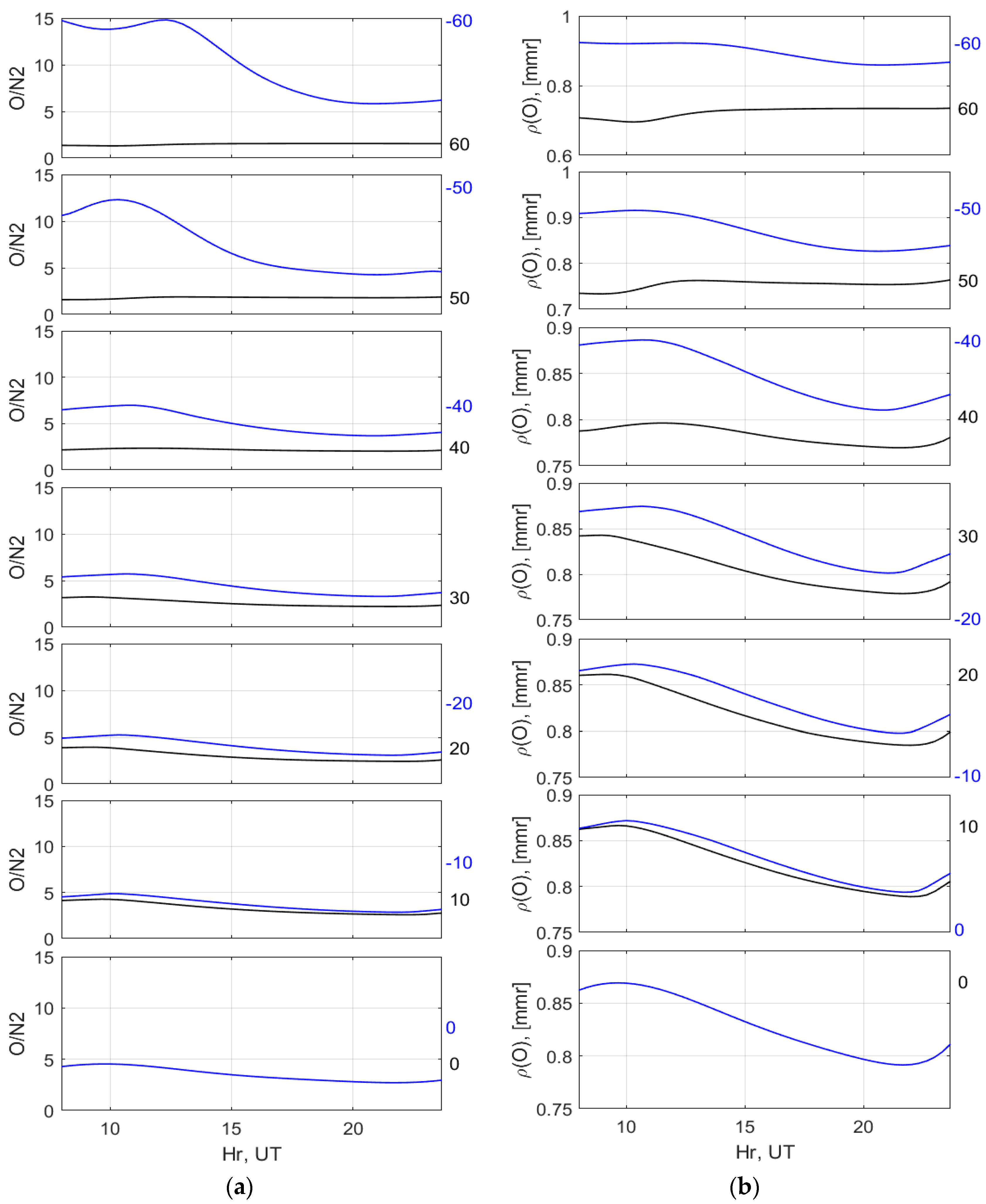
Figure 7 plots information on storm response for 26 August 2018, in a similar format to Figure 3, Figure 4 and Figure 5. The background TECo (top panel) on 26 August 2018 was very similar to that observed in the 27 May 2017 storm (compare to the top panel in Figure 3), with a clear asymmetry in TECo between the northern and southern hemispheres. Figure 7 (second panel) also shows some similarities with Figure 3 (second panel), including weak nighttime TIDs that mirrored the opposite hemisphere and prominent daytime TIDs in the SH versus the NH. However, what differs is the direction of propagation, which is not very clear for the August 2018 storm compared to the May 2017 storm. The mirrored MSTIDs are prominent at nighttime because electrodynamic processes are different from the daytime. In particular, with low E-region conductivity, the polarization electric field generated by the F-region wind dynamo is no longer short-circuited by the E region as during the day. Internal electric fields associated with MSTIDs in one hemisphere can be mapped to the conjugate hemisphere causing mirrored MSTID there. This nighttime MSTID conjugacy has been extensively discussed by [4,11]. Figure 7 (third panel) does not show clear TIDs as a function of longitude, as seen in Figure 3 (third panel), while the bottom panel shows similar simulated TEC asymmetry from TIEGCM.
Figure 8 and Figure 9 (top to bottom) are similar to Figure 4 and Figure 5 (top to bottom) but for geomagnetically quiet days of 24 and 25 August 2018. This is to show the consistency with 26 and 27 May 2017, which also represent quiet days. Figure 8 (bottom panel) also shows an example of TIEGCM simulation during quiet conditions. What is more conspicuous is the consistent enhanced TECo in the summer hemisphere (14:00–24:00 UT) as compared to observations on storm days (26 August 2018, and 28 May 2017). Similar consistency is seen in TIDs in the summer hemisphere, where high TECo is observed. The association of large amplitude TIDs with high plasma density (or TECo) is consistent throughout. To get a better picture of the correlation of TECo and TIDs, the ratio between TECo and TIDs is obtained, as shown in Figure 10. The left panels show the background TEC (TECo), TIDs, and the TIDs/TECo ratio for the SH. The right panels show the same parameters for the NH. The green lines on the TIDs/TECo ratio panels indicate the threshold that must be exceeded to be considered a strong occurrence of TIDs. It can be seen that where we have high TECo in the SH, we also have TIDs that greatly exceed the threshold, but that is not the case for the NH, where we have a low TECo, and a TIDs/TECo ratio mostly below the threshold. The figure also indicates that TIDs are attenuated at the equator as they travel northward, which is consistent with Figure 3 (second panel) and Figure 7 (second panel).

4. Discussion

4.1. Observed TEC Asymmetry

A prominent feature of both storm intervals presented here is a sharp hemispherical asymmetry in TECo. This behavior in two different solstice-time storms suggests a mechanism related to summer-to-winter background winds, which could produce a significant asymmetric storm effect on thermosphric composition and electron density.
In particular, the counter-electrojet (inferred from ∆H) on 28 May 2017 may be driven by the existence of a disturbance dynamo electric field (DDEF) caused by the earlier surge in the AE index (Figure 2). To verify whether this behavior can be repeated, we investigate another geomagnetic storm of similar magnitude that occurred on 26 August 2018, when similar behavior of the vertical plasma drift was observed, as mentioned in Section 3.3.
According to Abdu et al. [31] and Santos et al. [32], when the IMF Bz suddenly turns southward, convection electric fields become intensified in the magnetosphere and penetrate to the low-latitude ionosphere until such time as the plasmasphere is electrically shielded again. This penetrating electric field is known as an under-shielding electric field, with polarity in the dawn–dusk convection electric field. On the other hand, when the IMF Bz turns northward, causing a decline of convection electric fields, a strong over-shielding electric field becomes effective in the plasmasphere that has westward polarity on the day side and eastward polarity on the night side. The formation of DDEF due to geomagnetic storms can directly cause significant modifications of the vertical plasma drift of the equatorial and low-latitude ionosphere. These electric field effects are of long duration and are therefore qualitatively different from the preceding prompt penetration electric field (PPEF) and its attendant effects [33]. Both the PPEF and the DDEF could cause large-amplitude upward or downward drifts near the evening period and midnight hours, respectively [31,34,35].
The behavior of vertical drift as inferred from ∆H was not completely uniform in the storm intervals, being positive on both 26–27 May 2017, and 24–25 August 2018, from approximately 9:00 to 21:00 UT during the daytime period but negative on 28 May 2017, and 26 August 2018 during the same period. However, in both cases, TEC and electron density show a uniform enhanced response, as shown in Figure 3 (top panel) and Figure 7 (top panel). This is unexpected, because the resultant drift velocity should set the ionospheric plasma into motion [36]. Under normal circumstances, upward drift at the equatorial region is expected to lift plasma up across magnetic field lines at magnetic dip equator latitudes to altitudes where the plasma slowed down by pressure and gravity forces. The subsequent deposition of electron density at low latitudes should then symmetrically occur as the equatorial ionization anomaly (EIA). However, in both storm intervals (Figure 3 and Figure 7), we observed an asymmetry as enhancement of TECo in the SH, but a depletion in the NH. This result indicates that equatorial plasma fountain effects must be accompanied in these cases by significant variations in thermospheric composition and/or associated thermospheric neutral wind circulation. Furthermore, in both storm intervals presented here, the NH is the summer hemisphere and the SH is the winter hemisphere. Accordingly, normal quiet conditions should produce plasma density levels that are higher in the summer hemisphere at low latitudes, and such an effect is clearly seen in the quiet (non-storm) observations in Figure 4, Figure 5 and Figure 9 (top panels). However, this clearly did not occur during the two storm intervals, further indicating that thermospheric wind dynamics and O/N2 composition may be playing an important role in controlling storm response.

4.2. Mechanism Responsible for TECo and TID Asymmetry on Geomagnetically Disturbed Day

We investigate further the potential role of auroral energy input from both hemispheres in modulating presumed thermospheric wind and composition during storm conditions for the earlier 27 May 2017 storm. We first investigate the location of storm-time auroral source energy in both hemispheres by using two magnetometers located around the auroral region of SH and NH, respectively. Three magnetic components were used: magnetic north (N), magnetic east (E), and vertical down (Z). The T51 station is located at 48.05° N and 77.4° W (magnetic latitude: 57.0° N) in the north, and the AIA station is located at 65.3° S and 65.3° W (magnetic latitude: 55.5° S) in the south. Figure 11 (top panel) shows all the magnetic components from the NH for days 26–28 May 2017, and the bottom panel shows the magnetic components from the SH during the same days. A very large oscillation is clear in all the magnetic components for the magnetometer located in the NH (Figure 11, top panel), compared to a relatively small oscillation observed in the magnetometer located in the SH (Figure 11, bottom panel). This is very strong evidence that the energy input from the auroral source is higher in the NH than in the SH. Under these conditions, an enhanced convection of high latitude in the northern region will reinforce a southward neutral wind. Additionally, heating at high latitudes by the dissipation of electrical currents will create pressure gradients that drive an equatorward wind perturbation and in the process generate disturbance dynamo electric fields. A disturbance meridional wind can increase or lower the F region electron density peak height by moving ions and electrons up and down along magnetic field lines from high and middle latitudes to low latitudes. A TIEGCM model was used to provide disturbance time wind patterns (at 300 km altitude) that are useful for evaluating these potential mechanisms driving the asymmetry in TEC and TIDs in the SH.
Figure 12a shows that the TIEGCM modeled meridional winds are different during storm-time and quiet conditions. The disturbed condition shows overall southward winds, while the quiet condition shows overall northward winds. Figure 12b shows in more detail the TIEGCM-modeled meridional wind component as a function of latitude and time for conditions during the 27 May 2017 storm recovery phase. The blue and black lines represent meridional wind behavior in the SH and NH, respectively. We observe that the northward component of the wind starting from approximately 10:00 UT gradually turns southward as it propagates toward the equator. The southward component (blue line) of the wind on the other hand also travels northward but at lower amplitude compared to the northward component (black line). In other words, the SH meridional wind remains, while the wind in the NH travels toward the equator to the SH. This consistent with an overall summer-to-winter (northern-to-southern hemisphere) circulation.
If TIEGCM is correctly modeling the wind dynamics, wind perturbations are consistent with observations of observed enhanced density in the SH compared to the low density observed in the NH. In particular, stormtime meridional wind could change the neutral density composition, while wind from the source hemisphere (NH) would move O faster than N2 to the SH, since O is lighter than N2. Therefore, assuming that the downwelling of disturbed neutral composition would accordingly occur in the SH (winter hemisphere) during storms, O/N2 levels in the SH would be larger than in the NH, which in turn will enhance the plasma density, as observed in the SH. To verify this hypothesis, we examine TIEGCM model predictions of the O/N2 ratio and O in both hemispheres for stormtime conditions. Figure 13 shows that both O as well as O/N2 in the SH (blue line) are clearly higher than in the NH (black line). This high O/N2, resulting from a combined effect of stormtime and background solstice circulations, will contribute to enhanced ionospheric electron density in the southern hemisphere, as enhanced electron density is produced from higher O and/or reduced recombination occurs from lower N2. This implies that the observed larger density in the SH may be primarily a result of composition and wind circulation rather than the effect of electric field-induced drift. The work of Burns et al. [37] supports this conclusion, as that study showed that the modeled daytime geographical distribution increases the O/N2 ratio on a constant pressure surface in the low–middle latitudes of the winter hemisphere, and it tends to correspond very closely with the increase in the modeled electron densities at the F2 peak. However, further studies are necessary to establish the pattern of O/N2 with the electron density in the winter hemisphere during both geomagnetically disturbed and quiet periods.
A second possible explanation for the stronger TIDs in the SH is the so-called directional wind filter effect. Yeh et al. [38] noted that thermospheric wind acts as a directional filter at altitudes below the F2 peak due to effective wave reflection and trapping in the region. In general, thermospheric winds at any given location are the result of a complex set of forcing mechanisms including solar heating, high latitude energy, momentum deposition, and tides and waves propagating from lower atmosphere. Crowley and Rodrigues [39] show that a wave slowly moving in the same direction as a background wind is attenuated before reaching the ionosphere, while by contrast, a wave traveling faster and in the opposite direction to the wind would propagate to the ionosphere. This hypothesis is supported by our observations in Figure 3 (wave parameter) and Figure 12b (wind parameter). Specifically, the winds at −60 to approximately 0 degrees (geographic latitudes and −66.1 to −7.4 degree geomagnetic latitudes) are southward (Figure 12b), while the TIDs at −30 to 0 degrees (geomagnetic and −40 to −7 geography) are northward (Figure 3). Therefore, the wind and the waves are traveling in opposite directions, which is consistent with the wind filtering theory mentioned by Cowling et al. [21] and Crowley and Rodrigues [39]. Under these conditions, waves (TIDs) can propagate with larger amplitudes, which is consistent with the observations shown in Figure 3 (second panel) at 12:00 UT to 15:00 UT. On the other hand, when the wind is northward around approximately 40 degrees (geographic north and approximately 30 degrees geomagnetic north), TIDs in the same region are also propagating northward, but they are attenuated, as seen in Figure 3 (second panel) from 12:00 UT to 21:00 UT. This is in line with the directional filter effect explained above and could explain why we observe weak TIDs in the NH compared to the SH in the second panel of Figure 3 and Figure 7.
Our discussion so far is based on geographic meridional winds, and wind-induced plasma motion as in TIDs is confined to be field aligned. Therefore, at locations where magnetic declination is large, geographic zonal winds can make an important additional contribution to ionospheric electron density variations e.g., [40]. In order to gauge the potential contribution of zonal winds during the two studied storms, we also plot TIEGCM magnetic meridional winds in Figure 12c. Outside of cases with greatly amplified zonal winds (not characteristic of the two storms studied here), the zonal wind effect is mostly dependent on the value of declination, which in the American sector is very large in the southern hemisphere and modest at northern middle latitudes. Therefore, this explanation without applying the magnetic meridional wind component (i.e., Figure 12b) is sustainable even with the contribution of the zonal wind effect.
Another noticeable behavior of the northward meridional wind component (in Figure 12b, black line) is the change in direction around 15:00 UT to 21:00 UT at 60 to 20 degree latitude north. This change in direction can also be observed in the TIDs (in Figure 3, second panel) around the same time period. The coincidence in wind and TIDs directional change needs further investigation, which can be carried out in future studies
Finally, the asymmetrical TIDs observed in the SH around 12:00–21:00 UT in Figure 3 and Figure 7 during the two storm events have multiple potential sources. In particular, they may be generated either in the NH and grow in amplitude as they encounter larger plasma density in the SH, or they are locally generated in the SH and attenuate as they travel northward to the NH due to the directional wind filter effect. Future expanded stormtime case studies for different seasons are necessary to further clarify these TID characteristics.

5. Conclusions

A number of factors can affect the TID propagation, including the TID amplitude attenuation. This study, based on two northern summer geomagnetic storms cases, demonstrates two of these important factors. The first is relevant to a positive correlation between TID wave amplitude and background ionospheric density [1]; i.e., ΔNe/Ne is determined primarily by atmospheric gravity wave (AGW) neutral disturbance properties as in the AGW dispersion and polarization relations. On the other hand, to make the Ne effect more complicated, high electron density provides elevated damping on TID amplitudes, which may be non-negligible. Thus, with high electron density near the equatorial ionization anomaly region, it is of interest to explore how TID amplitudes vary across the region. The second factor is the wind filtering effect. As described earlier, the background neutral winds may or may not favor the horizontal propagation of TIDs. It should be noted that stormtime disturbance winds (equatorward) have not been consistently monitored with large spatial coverage, and thus the observations of TIDs may provide important information on these winds. The two geomagnetic storms we investigated occurred in the summer took place on 27 May 2017 and 25 August 2017. In addition to GNSS TID analysis, we also use swarm electron density in situ measurements and TIEGCM model simulations to assist in our TID interpretation.
We showed very consistent features such as higher Ne density and stronger TIDs (in amplitude) in the low-latitude southern hemisphere as compared to the northern hemisphere. [O/N2], and the meridional neutral wind component from TIEGCM is used to explain higher electron density and strong TIDs in the SH. Observed TID variations are connected to stormtime modifications in background electron density, neutral wind, and/or O/N2. Additionally, we showed that the meridional component of the neutral wind during geomagnetically disturbed days can play an important role in TID propagation. This conclusion is important, as TID activity in the ionosphere can be significant in the transfer of energy and momentum from one atmospheric region to another. Finally, we demonstrated that background TEC density can have a strong modifying influence on stormtime TID amplitudes, since larger plasma density is correlated with larger TID amplitude and vice versa.

Author Contributions

Conceptualization, O.F.J. and S.Z.; methodology, O.F.J.; software, O.F.J. and W.R.; validation, S.Z., A.J.C., P.J.E., L.P.G., E.R.d.P. and R.d.J.; formal analysis, O.F.J.; investigation, O.F.J. and S.Z.; resources, A.J.C. and P.J.E.; data curation, W.R.; writing—original draft preparation, O.F.J.; writing—review and editing, O.F.J., S.Z., P.J.E.; visualization, E.R.d.P., L.P.G. and R.d.J.; supervision, S.Z. and P.J.E.; project administration, A.J.C. and P.J.E.; funding acquisition, P.J.E. All authors have read and agreed to the published version of the manuscript.

Funding

This research was funded by US National Science Foundation grant AGS-1242204, NASA LWS grant NNX15AB83G, AFOSR MURI grant support FA9559-16-1-0364 and ONR grant N00014-17-1-2186.

Acknowledgments

GPS TEC data products and access through the Madrigal distributed data system are provided to the community (http://www.openmadrigal.org) by the Massachusetts Institute of Technology (MIT). Data for TEC processing is provided from the following organizations: UNAVCO, Scripps Orbit, Permanent Array Center, Institut Geographique National, France, International GNSS Service, The Crustal Dynamics Data Information System (CDDIS), National Geodetic Survey, Instituto Brasileiro de Geografia e Estatística, RAMSAC CORS of Instituto Geográfico Nacional de la República Argentina, Arecibo Observatory, Low-Latitude Ionospheric Sensor Network (LISN), Topcon Positioning Systems, Inc., Canadian High Arctic Ionospheric Network, Centro di Ricerche Sismologiche, Système d’Observation du Niveau des Eaux Littorales (SONEL), RENAG: REseau NAtional GPS permanent, GeoNet—the official source of geological hazard information for New Zealand, GNSS Reference Networks, Finnish Meteorological Institute, and SWEPOS of Sweden. Access to these data is provided by the Madrigal network via: http://cedar.openmadrigal.org/. E. R. de Paula acknowledges the support of CNPq through Grant 310802/2015-6 and INCT GNSS-NavAer Grants 2014/465648/2014-2 CNPq and 2017/50115-0 FAPESP. The authors thank E. Yizengaw, C. E Valladares, and the rest of the AMBER and LISN teams for the magnetometer data. AMBER is operated by Boston College with funding from NASA and AFOSR. Data are available at: http://magnetometers.bc.edu/. LISN is a project led by the University of Texas at Dallas in collaboration with the Geophysical Institute of Peru and other institutions that provide information for the benefit of the scientific community. Data are available at http://lisn.igp.gob.pe. We also acknowledge SGS, Jeffrey J. Love; CARISMA, PI Ian Mann; CANMOS; The S-RAMP Database, PI K. Yumoto and K. Shiokawa; The SPIDR database; AARI, PI Oleg Troshichev; The MACCS program, PI M. Engebretson, Geomagnetism Unit of the Geological Survey of Canada; GIMA; MEASURE, UCLA IGPP and Florida Institute of Technology; SAMBA, PI Eftyhia Zesta; 210 Chain, PI K. Yumoto; SAMNET, PI Farideh Honary; The institutes who maintain the IMAGE magnetometer array, PI Eija Tanskanen; PENGUIN; AUTUMN, PI Martin Connors; DTU Space, PI Dr. Rico Behlke; South Pole and McMurdo Magnetometer, PI’s Louis J. Lanzarotti and Alan T. Weatherwax; ICESTAR; RAPIDMAG; PENGUIn; British Artarctic Survey; McMac, PI Peter Chi; BGS, PI Susan Macmillan; Pushkov Institute of Terrestrial Magnetism, Ionosphere and Radio Wave Propagation (IZMIRAN); GFZ, PI Juergen Matzka; MFGI, PI B. Heilig; IGFPAS, PI J. Reda; University of L’Aquila, PI M. Vellante; BCMT, V. Lesur and A. Chambodut; Data obtained in cooperation with Geoscience Australia, PI Marina Costelloe; SuperMAG, PI Jesper W. Gjerloev. Data from SuperMag network can be downloaded at: http://supermag.jhuapl.edu/mag/?stations=GIM&tab=stations&start=2017-05-28T00%3A00%3A00.000Z&interval=23%3A59. Simulation data have been provided by the Community Coordinated Modeling Center at Goddard Space Flight Center through their public Runs on Request system (http://ccmc.gsfc.nasa.gov). The TIEGCM Model was developed by the R. G. Roble et al at the High Altitude Observatory of the National Center for Atmospheric research.

Conflicts of Interest

The authors declare no conflict of interest.

References

  1. Hines, C.O. Internal atmospheric gravity waves at ionospheric heights. Can. J. Phys. 1960, 38, 1441–1481. [Google Scholar] [CrossRef]
  2. Hunsucker, R.D. Atmospheric gravity waves generated in the high latitude ionosphere: A review. Rev. Geophys. 1982, 20, 293–315. [Google Scholar] [CrossRef]
  3. Jonah, O.F.; Kherani, E.A.; de Paula, E.R. Observation of TEC perturbation associated with medium-scale traveling ionospheric disturbance and possible seeding mechanism of atmospheric gravity wave at a Brazilian sector. J. Geophys. Res. 2016, 121, 2531–2546. [Google Scholar] [CrossRef] [Green Version]
  4. Jonah, O.F.; Kherani, E.A.; De Paula, E.R. Investigations of conjugate MSTIDS over the Brazilian sector during daytime. J. Geophys. Res. Space Phys. 2017, 122. [Google Scholar] [CrossRef]
  5. Frissell, N.A.; Baker, J.B.H.; Ruohoniemi, J.M.; Gerrard, A.J.; Miller, E.S.; Marini, J.P.; West, M.L.; Bristow, W.A. Climatology of medium-scale traveling ionospheric disturbances observed by the midlatitude Blackstone SuperDARN radar. J. Geophys. Res. 2014, 119, 7679–7697. [Google Scholar] [CrossRef]
  6. Jonah, O.F.; Coster, A.; Zhang, S.; Goncharenko, L.; Erickson, P.J.; de Paula, E.R.; Kherani, E.A. TID observations and source analysis during the 2017 Memorial Day weekend geomagnetic storm over North America. J. Geophys. Res. Space Phys. 2018, 123. [Google Scholar] [CrossRef]
  7. MacDougall, J.W.; Jayachandran, P.T. Spaced transmitter measurements of medium scale traveling ionospheric disturbance near equator. Geophys. Res. Lett. 2011, 38, L16806. [Google Scholar] [CrossRef] [Green Version]
  8. Jonah, O.F. A Study of Daytime MSTIDS over Equatorial and Low Latitude Regions during Tropospheric Convection: Observations and Simulations, The Graduate Course in Space Geophysics. Ph.D. Thesis, National Institute for Space Research (INPE) Sao Jose dos Campos, Sao Paulo, Brazil, 2017. [Google Scholar]
  9. Davis, M.J.; Ross, A.V. Traveling Ionospheric Disturbances Originating in the Auroral Oval during Polar Substorms. J. Geophys. Res. 1969, 74, 5721–5735. [Google Scholar] [CrossRef]
  10. MacDougall, J.W.; Li, G.; Jayachandran, P.T. Traveling ionospheric disturbances near London. Can. J. Atmos. Sol. Terr. Phys. 2009, 71, 2077–2084. [Google Scholar] [CrossRef]
  11. Otsuka, Y.; Shiokawa, K.; Ogawa, T.; Wilkinson, P. Geomagnetic conjugate observations of medium-scale traveling ionospheric disturbances at midlatitude using all-sky airglow imagers. Geophys. Res. Lett. 2004, 31, L15803. [Google Scholar] [CrossRef]
  12. Tsugawa, T.; Otsuka, Y. A statistical study of large-scale traveling ionospheric disturbances using the GPS network in Japan. J. Geophys. Res. 2004, 109, A06302. [Google Scholar] [CrossRef]
  13. Afraimovich, E.L.; Kosogorov, E.A.; Leonovich, L.A.; Palamarchouk, K.S.; Perevalova, N.P.; Pirog, O.M. Determining parameters of large-scale traveling ionospheric disturbances of auroral origin using GPS-arrays. J. Atm. Sol. Ter. Phys. 2000, 62, 553–565. [Google Scholar] [CrossRef]
  14. Kil, H.; Paxton, L.J. Global distribution of nighttime medium-scale traveling ionospheric disturbances seen by Swarm satellites. Geophys. Res. Lett. 2017, 44, 9176–9182. [Google Scholar] [CrossRef]
  15. Habarulema, J.B.; Yizengaw, E.; Katamzi-Joseph, Z.T.; Moldwin, M.B.; Buchert, S. Storm time global observations of large scale TIDs from ground-based and in situ satellite measurements. J. Geophys. Res. Space Phys. 2018, 123, 711–724. [Google Scholar] [CrossRef] [Green Version]
  16. Candido, C.M.N.; Pimenta, A.A.; Bittencourt, J.A.; Beckerguedes, F. Statistical analysis of the occurrence of medium-scale traveling ionospheric disturbances over Brazilian low latitudes using OI 630.0 nm emission all-sky images. Geophys. Res. Lett. 2008, 35. [Google Scholar] [CrossRef] [Green Version]
  17. Coster, A.J.; Goncharenko, L.; Zhang, S.; Erickson, P.J.; Rideout, W.; Vierinen, J. GNSS observations of ionospheric variations during the 21 August 2017 solar eclipse. Geophy. Res. Lett. 2017, 17, 349–352. [Google Scholar] [CrossRef] [Green Version]
  18. Ngwira, C.M.; Habarulema, J.B.; Astafyeva, E.; Yizengaw, E.; Jonah, O.F.; Crowley, G.; Gisler, A.; Coffey, V. Dynamic response of ionospheric plasma density to the geomagnetic storm of 22–23 June 2015. J. Geophys. Res. Space Phys. 2019, 124. [Google Scholar] [CrossRef]
  19. Tsugawa, T.; Otsuka, Y.; Coster, A.J.; Saito, A. Medium-scale traveling ionospheric disturbances detected with dense and wide TEC maps over North America. Geophys. Res. Lett. 2007, 34, L22101. [Google Scholar] [CrossRef]
  20. Zhang, S.; Erickson, P.J.; Goncharenko, L.; Coster, A.J.; Rideout, W.; Vierinen, J. Ionospheric bow waves and perturbations induced by the 21 august 2017 solar eclipse. Geophys. Res. Lett. 2017, 44, 12–67. [Google Scholar] [CrossRef] [Green Version]
  21. Cowling, D.H.; Webb, D.; Yeh, K.C. Group Rays of Internal Gravity Waves in a Wind-Stratified Atmosphere. J. Geophys. Res. 1971, 76, 213–220. [Google Scholar] [CrossRef]
  22. Waldock, J.A.; Jones, T.B. The effects of neutral winds on the propagation of medium-scale atmospheric gravity waves at mid-latitudes. J. Atm. Terr. Phys. 1983, 46, 217–231. [Google Scholar] [CrossRef]
  23. Vasseur, G. Dynamics of the F-region observed with Thomson scatter. J. Atmos. Terr. Phys. 1969, 31, 397–420. [Google Scholar] [CrossRef]
  24. Fujiwara, H.; Maeda, S.; Fukunishi, H.; Fuller-Rowell, T.J.; Evans, D.S. Global variations of thermospheric winds and temperatures caused by substorm energy injection. J. Geophys. Res. Space Phys. 1996, 101, 225–239. [Google Scholar] [CrossRef]
  25. Fuller-Rowell, T.J.; Codrescu, M.V.; Moffett, R.J.; Quegan, S. Responses of the thermosphere and ionosphere to geomagnetic storms. J. Geophys. Res. Space Phys. 1994, 99, 3893–3914. [Google Scholar] [CrossRef]
  26. Blanc, M.; Richmond, A.D. The ionospheric disturbance dynamo. J. Geophys. Res. 1980, 85, 1669–1686. [Google Scholar] [CrossRef]
  27. Rideout, W.; Coster, A. Automated GPS processing for global total electron content data. GPS Solut. 2006, 10, 219–228. [Google Scholar] [CrossRef]
  28. Vierinen, J.; Coster, A.J.; Rideout, W.C.; Erickson, P.J.; Norberg, J. Statistical framework for estimating GNSS bias. Atmos. Meas. Tech. Discuss. 2017, 8, 9373–9398. [Google Scholar] [CrossRef] [Green Version]
  29. Zhang, S.R.; Coster, A.J.; Erickson, P.J.; Goncharenko, L.P.; Rideout, W.; Vierinen, J. Traveling Ionospheric Disturbances and Ionospheric Perturbations Associated with Solar Flares in September 2017. J. Geophys. Res. Space Phys. 2019, 60, 895. [Google Scholar] [CrossRef] [Green Version]
  30. Roble, R. The NCAR thermosphere-ionosphere-mesophere-electrodynamics general circulation model (TIME-GCM). In Solar-Terrestrial Energy Program: Handbook of Ionospheric Models; Schunk, R., Ed.; Utah State University: Logaan, UT, USA, 1996; pp. 281–288. [Google Scholar]
  31. Abdu, M.A.; Kherani, E.A.; Batista, I.S.; Sobral, J.H.A. Equatorial evening prereversal vertical drift and spread F suppression by disturbance penetration electric fields. Geophys. Res. Lett. 2009, 36. [Google Scholar] [CrossRef] [Green Version]
  32. Santos, A.M.; Abdu, M.A.; Souza, J.R.; Sobral, J.H.A.; Batista, I.S. Disturbance zonal and vertical plasma drifts in the Peruvian sector during solar minimum phases. J. Geophys. Res. Space Phys. 2016, 121. [Google Scholar] [CrossRef] [Green Version]
  33. Abdu, M.A.; de Souza, J.R.; Sobral, J.H.A.; Batista, I.S. Magnetic storm associated disturbance dynamo effects in the low and equatorial latitude ionosphere, in Recurrent Magnetic Storms: Corotating Solar Wind Streams. Geophys. Monogr. Ser. 2006, 167, 283–304. [Google Scholar] [CrossRef]
  34. Richmond, A.D.; Peymirat, C.; Roble, R.G. Long-lasting disturbances in the equatorial ionospheric electric field simulated with a coupled magnetosphere-ionosphere-thermosphere model. J. Geophys. Res. 2003, 108, 1118. [Google Scholar] [CrossRef]
  35. Sobral, J.H.A.; Abdu, M.A.; Gonzalez, W.D.; Gonzalez, A.C.; Tsurutani, B.T.; Da Silva, R.R.; Barbosa, I.G.; Arruda, D.C.; Denardini, C.M.; Zamlutti, C.J.; et al. Equatorial ionospheric responses to high intensity long-duration auroral electrojet activity (HILDCAA). J. Geophys. Res. 2006, 111, A07S02. [Google Scholar] [CrossRef] [Green Version]
  36. Kelley, M.C. The Earth’s Ionosphere; Academic Press: London, UK, 1989. [Google Scholar]
  37. Burns, A.G.; Killeen, T.L.; Deng, W.; Carignan, G.R.; Roble, R.G. Geomagnetic storm effects in the low- to middle-latitude upper thermosphere. J. Geophys. Res. 1995, 100, 14673–14691. [Google Scholar] [CrossRef]
  38. Yeh, K.C.; Webb, H.D.; Cowling, D.H. Evidence of Directional Filtering of Traveling Ionospheric Disturbances. Nat. Phys. Sci. 1972, 235, 131–132. [Google Scholar] [CrossRef]
  39. Crowley, G.; Rodrigues, F.S. Characteristics of traveling ionospheric disturbances observed by the TIDDBIT sounder. Radio Sci. 2012, 47, 1–12. [Google Scholar] [CrossRef]
  40. Zhang, S.R.; Foster, J.C.; Holt, J.M.; Erickson, P.J.; Coster, A.J. Magnetic declination and zonal wind effects on longitudinal differences of ionospheric electron density at midlatitudes. J. Geophys. Res. Space Phys. 2012, 117, A08329. [Google Scholar] [CrossRef] [Green Version]
Figure 1. (a) An example of ionospheric pierce point distribution of the total electron content (TEC) measurement on 8 May 2017 at 10:00 UT. The black line represents the magnetic equator. (b) Examples of traveling ionospheric disturbances (TID) analysis procedures. The blue line represents the background TEC from one station and two satellites, the red line represents the hourly sliding window using the Savityky–Golay low-pass filter, and the back line represents the differential TEC (∆TEC).
Remotesensing 12 00228 g001aRemotesensing 12 00228 g001b
Figure 2. Geophysical and geomagnetic conditions during 26–28 May 2017. From top to bottom: solar wind speed (Vsw), the Bz component of the magnetic field of interplanetary magnetic field (IMF), the symmetric magnetic field strength (Sym-H) index, the auroral electrojet (AE) index, ∆H(Belem − Petrolina), interplanetary east–west electric field (Ey, positive to east), and the Kp magnetic index. The dashed lines represent the time period when different features of TIDs were observed. The black circle (on the ∆H panel) highlights the ∆H downward plasma drift on 28 May 2017.
Remotesensing 12 00228 g002
Figure 3. From top to bottom: keogram of background GNSS-TEC; on the right is the electron density obtained from the SWARM B satellite; keogram of TID obtained by removing the background TEC as a function of latitude and local and universal time (longitude: 55–65° S); keogram of TID as a function of longitude, local, and universal time on 28 May 2017; and the simulation of TEC using the thermosphere–ionosphere–electrodynamics general circulation model (TIEGCM) (at ±30° geomagnetic latitudes).
Remotesensing 12 00228 g003
Figure 4. The same plots as Figure 3, but for a quiet day: 27 May 2017.
Remotesensing 12 00228 g004
Figure 5. The same plots as Figure 3, but for a quiet day: 26 May 2017. The dashed lines on the bottom panel are determined by tracking the pack to pack of each wave using visual assessment.
Remotesensing 12 00228 g005
Figure 6. Geophysical and geomagnetic conditions during 24–27 August 2018. From top to bottom: solar wind speed (Vsw), the Bz component of the magnetic field of interplanetary magnetic field (IMF), the Sym-H index, the ∆H(Jica – Piur), interplanetary east–west electric field (Ey, positive to east), and the Kp magnetic index. The dashed lines represent the time period when different features of TIDs were observed. The black circle on the ∆H panel higlights when the ∆H turned downward on 26 August 2018 with some intermittent oscillations.
Remotesensing 12 00228 g006
Figure 7. From top to bottom: keogram of background GNSS-TEC, keogram of TID obtained by removing the background TEC as a function of latitude and local and universal time, a keogram of TID as a function of longitude and local and universal time on 26 August 2018, and the simulation of TEC using the TIEGCM (at ±30° geomagnetic latitudes).
Remotesensing 12 00228 g007
Figure 8. The same plots as Figure 8, but for 25 August 2018.
Remotesensing 12 00228 g008
Figure 9. The same plots as Figure 8, but for 24 August 2018.
Remotesensing 12 00228 g009
Figure 10. The left panels show the background TEC (TECo), TIDs, and TIDs/TECo for the southern hemisphere, and the right panels show the same parameters for the northern hemisphere. All the parameters (except for the parameter represented by the bottom panels) are represented in TECU where 1 TECu = 1016 electron/m2.
Remotesensing 12 00228 g010
Figure 11. The top panel shows values of magnetic north, east, and vertical components during 26–28 May 2017 for the T51 magnetometer station located in the northern hemisphere (48.05° N, 77.4° W, Mlat: 57.0° N). The bottom panel shows values of magnetic north, east, and vertical components during 26–28 May 2017 for the AIA magnetometer station located in the southern hemisphere (65.3° S, 65.3° W, M.lat: 55.5° S).
Remotesensing 12 00228 g011
Figure 12. (a) Contour map for the meridional positive northward wind for both disturbed (top panel) and quiet (bottom panel) days. (b) TIEGCM result for 28 May 2017, showing meridional wind velocity changing from northward to southward geographically. (c) Same as (b) but in the magnetic meridian coordinate. The blue line represents the component of the wind in the south (0 to −60 degrees), and the black line represents the component of the winds in the north (0 to 60 degrees). The positive value of the winds indicates northward.
Remotesensing 12 00228 g012aRemotesensing 12 00228 g012b
Figure 13. TIEGCM-simulated O/N2 ratio (a) and O (b) at a fixed longitude of 65° W. The blue line represents the O and O/N2 ratio in the southern hemisphere (SH). The black lines represent the O and O/N2 ratio in the northern hemisphere (NH).
Remotesensing 12 00228 g013

