Breaking Wave Height Estimation from Timex Images: Two Methods for Coastal Video Monitoring Systems

Abstract

The breaking wave height is a crucial parameter for coastal studies but direct measurements constitute a difficult task due to logistical and technical constraints. This paper presents two new practical methods for estimating the breaking wave height from digital images collected by shore-based video monitoring systems. Both methods use time-exposure (Timex) images and exploit the cross-shore length ($L_{Hs}$) of the typical time-averaged signature of breaking wave foam. The first method ($H{s}_{b,v}$) combines $L_{Hs}$ and a series of video-derived parameters with the beach profile elevation to obtain the breaking wave height through an empirical formulation. The second method ($H{s}_{b,v24}$) is based on the empirical finding that $L_{Hs}$ can be associated with the local water depth at breaking, thus it can be used to estimate the breaking wave height without the requirement of local bathymetry. Both methods were applied and verified against field data collected at the Portuguese Atlantic coast over two days using video acquired by an online-streaming surfcam. Furthermore, $H{s}_{b,v24}$ was applied on coastal images acquired at four additional field sites during distinct hydrodynamic conditions, and the results were compared to a series of different wave sources. Achievements suggest that $H{s}_{b,v}$ method represents a good alternative to numerical hydrodynamic modeling when local bathymetry is available. In fact, the differences against modeled breaking wave height, ranging from 1 to 3 m at the case study, returned a root-mean-square-error of 0.2 m. The $H{s}_{b,v24}$ method, when applied on video data collected at five sites, assessed a normalized root-mean-square-error of 18% on average, for dataset of about 900 records and breaking wave height ranging between 0.1 and 3.8 m. These differences demonstrate the potential of $H{s}_{b,v24}$ in estimating breaking wave height merely using Timex images, with the main advantage of not requiring the beach profile. Both methods can be easily implemented as cost-effective tools for hydrodynamic applications in the operational coastal video systems worldwide. In addition, the methods have the potential to be coupled to the numerous other Timex applications for morphodynamic studies.

1. Introduction

The wave height at the breaking point (hereafter the breaking wave height) is an essential component in any study regarding coastal processes. Examples include the estimation of the longshore drift (e.g., [1]), the design of coastal structures (e.g., [2]) and the coastal risk assessment (e.g., [3]).

When offshore waves propagate into shallower water depths, the wave steepness increases and wave profiles become skewed and asymmetric. When the wave height is approximately equal to the water depth, the wave breaking phenomenon occurs (e.g., [4]). The wave form at breaking can be characterized into four types, namely surging, collapsing, spilling, and plunging breakers, based on the Iribarren number (e.g., [4]). For surging and collapsing wave forms, the wave crest remains unbroken while the shoreward wave face breaks slightly. In spilling breaking, the wave crest spills down the face of the wave. Plunging breakers are the most energetic, with the wave crest and face completely collapsing and plunging into the wave trough. The breaking wave form, and consequently the breaking location, is mainly determined by the beach slope and the offshore wave steepness (e.g., [5,6]).

Direct measurements of the breaking wave height are logistically complex, especially during storm conditions and where morphological changes can prevent the recovery of oceanographic instrumentation. As a consequence, breaking wave height is usually derived with process-based numerical models (e.g., SWAN [7] and SWASH [8]) or by empirical relationships [9,10], both of which usually require a nearshore topo-bathymetric profile that is often difficult to obtain with adequate temporal and spatial resolution. In addition, numerical models and empirical relationships often lack accuracy when applied on the field [11]. This can be associated with the description of the breaking wave mechanism which may not account for all the physical processes involved, such as nonlinear wave–wave interactions [4], wave–current interactions [12], and wave reflection [6], the latter being found to influence the variation of wave height to water depth ratio [13].

Coastal video monitoring is a shore-based remote sensing technique that uses images acquired by optical devices installed on an elevated position collecting high-frequency frames of the nearshore area [14,15,16]. The video monitoring technique has been proven as a valid tool for measuring wave breaking height because the wave characteristics have a visible signature on the sea surface. Existing video-based methods for estimating breaking wave height are based on the use of Timestack images [17,18], which are obtained by sampling and concatenating a single transect of pixel from each image over a given interval of time [19]. These methodologies exploit the photogrammetric relation between the camera location and incipient breaking point visible on Timestacks [17,18]. Nevertheless, the fundamental image processing procedures dedicated to the identification of the breaking point require a pixel intensity threshold calibration based on image pixel quality [17], and are limited to those specific hydrodynamic conditions in which the breaking point is clearly identifiable on images [18,20]. Huntley et al. [21] proposed an alternative solution using a so-called “Brightest” image, which is formed by the highest pixel intensity over a sampling interval.

Considering that the production of Timestacks and Brightest images is not often set routinely by the coastal video systems installed worldwide, a methodology based on the use of the most common images produced by coastal video monitoring systems, namely Time-Exposure images (hereinafter, Timex images), would be beneficial. Timex images are generated by the average of the individual images collected over a sampling period, usually 10 min [16,19]. The main characteristic of Timex is to show a time-averaged white pixel pattern at the breaking location, usually associated with the wave energy dissipation process over a bar crest and/or at the shore [22,23].

This work proposes two practical methods to estimate the breaking wave height from Timex video images. Video data collected on a field site were used to set up the methods. The statistical location of incipient breaking points on a 10-min Timestack image is used as preliminary analysis to relate wave breaking fraction to the pixel intensity pattern on Timex images. The first method ($H{s}_{b,v}$) combines Timex-derived pixel statistical parameters and the beach profile with an empirical model. The second method ($H{s}_{b,v24}$) aims to provide a video-based approach that does not require a beach profile.

The paper is structured as follows. Section 2.1 introduces the field case study and video data. By exploiting the properties of Timestack image, we found a relationship between incipient breaking points location and image pixel intensity (Section 2.2). Section 2.3 presents the conceptualization of the first method ($H{s}_{b,v}$), an empirical formulation combining video-derived parameters and beach profile elevation to estimate wave breaking height. Section 2.4 describes the algorithm that was developed to automatically extract the parameters to solve $H{s}_{b,v}$. The video-derived parameters found at the case study are shown in Section 2.5, and their analysis leads to develop the second method ($H{s}_{b,v24}$) in Section 2.6. In Section 2.7, four additional field sites are introduced to apply $H{s}_{b,v24}$ with different hydrodynamic conditions. Section 3 reports the results for both methods. Section 4 discusses the assessments and underlines the limitations of each presented method, Section 5 summarizes the main findings.

2. Methods

2.1. Case Study

2.1.1. Site and Video Data

To set up and verify the methods developed in this work, we used the images acquired by an online streaming camera at Ribeira d’Ilhas beach (38°59′17.0″N, 9°25′10.4″W), located on the Portuguese western coast facing the North Eastern Atlantic Ocean (Figure 1). The beach extends for about 300 m cross-shore, with a NW–SE orientation. It is limited by a 55-m cliff southward, and by a small headland in the north. The nearshore profile develops over a rocky shore platform with an almost-planar slope (tanβ = 0.005) in the intertidal range of 0 ± 1.5 m depth, increasing up to tanβ = 0.03 in the supratidal range 1.5 ± 5.5 m (Figure 1). The tidal regime is mesotidal, with an average tidal range of 2.10 m [24].

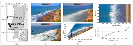
Figure 1. Study site and video data. (a) Geographic location of Ribeira d’Ilhas beach (black square), Monican buoy (circle), and Cascais tide gauge (diamond). (b) The 10-min Timex images produced during low tide (top) and high tide (bottom). Symbols show pressure transducers array in the intertidal area, dashed black line represents the transect used to produced Timestack images. (c) Examples of oblique (top) and rectified (bottom) Timex. Dashed black line represents the transect used to produced Timestack images. (d) Timestack image example (top) and corresponding beach profile (bottom). The profile also corresponds to the transect sampled on Timex to retrieve I_TX.

The camera is an online streaming Internet Protocol (IP) device installed by the company Surftotal (www.surftotal.com) on the roof of a house, at an elevation of about 80 m above Mean Sea Level (MSL) and at a distance of 400 m from the shore. Image frames (image size 800 × 450) were extracted from the video burst at 5 Hz to generate 10-min Timex images for two days, 28 and 29 March 2017 (Figure 1). Images were rectified at the corresponding water level [14,25] with a spatial image resolution of 1 m² pixel footprint. Ten-minute Timestack images were also produced along the cross-shore transect perpendicular to the wave propagation direction, with 1 m spatial and 1 s temporal resolution (Figure 1). The final dataset consisted of 52 and 42 Timex-Timestacks images for the first (28 March) and second days (29 March) of video acquisition, respectively.

2.1.2. Hydrodynamics

During the video acquisition, four synchronized pressure transducers (PTs) were deployed near the bottom in the intertidal section of the profile. The pressure data of the most seaward PT were used to obtain the mean sea level (MSL), which varied between a minimum of −0.94 m and a maximum of 1.8 m above MSL during both days (Figure 2). Offshore wave data were provided by the Portuguese Hydrographic Institute (www.hidrografico.pt), recorded by the Monican buoy deployed at 80 m depth (Figure 1). While on 28 March the wave conditions were approximately constant (offshore wave height Ho = 1.7 m, wave peak period Tp = 11.5 s), on 29 March the Ho increased from about 2.0 to 3.5 m and Tp decreased from 18 to 16.5 s. In the intertidal zone, significant wave height Hs (derived from PTs using linear wave theory [26]) was depth-dependent due to the wave energy dissipation by the depth-induced breaking process. Wave period timeseries derived from PTs records was in agreement with measures provided by the offshore buoy.

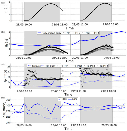
Figure 2. Hydrodynamic conditions during the experience: (a) water level η measured by the most seaward PT; (b) significant wave height $H_s$ measured by Monican buoy (blue line) and PTs (symbols) in the intertidal area; (c) wave period from buoy (lines) and from PTs (symbols); and (d) wave direction from buoy. Gray rectangles indicate the intervals in which video data are available.

Nearshore and breaking wave conditions were obtained using the SWAN and SWASH models, respectively. In particular, the SWAN model was used to propagate waves from offshore up to 20 m depth, while SWASH model was used for wave propagation from 20 m up to the shore.

SWAN was run in nested mode, with an offshore domain (78 km × 84 km) with 1000 m spatial resolution, with its upper left corner coincident with the Monican buoy location (Figure 1a), and a nearshore domain (9.8 km × 10.3 km) with 100 m spatial resolution, from approximately 70 to 20 m depth. Offshore boundary conditions were specified at the northern, western, and southern boundaries using the wave parameters (Hs, Tp, and PDir) measured by the Monican buoy assuming a JONSWAP type spectrum with γ = 3.3. Wind was not considered in the SWAN computational domain, as wave conditions during the field campaign were mainly associated with swell conditions (Figure 2c). The physical processes that were activated in the SWAN simulation were nonlinear wave interactions (triads), wave energy dissipation by bottom friction (JONSWAP default parameterization) and by depth-induced breaking ([27] default parameterization).

The SWASH numerical model [8] was used to estimate the Hs variation over the chosen Timestack profile (Figure 1d). Boundary conditions were specified at 20 m water depth using the wave parameters (Hs, Tp) obtained from the SWAN simulation with a JONSWAP type spectrum (γ = 3.3). A weakly-reflective boundary condition was applied at the offshore boundary and tide level was based on Cascais tide gauge (available at ftp://ftp.dgterritorio.pt/Maregrafos/Cascais). The SWASH grid was constructed with a cross-shore grid size of 1 m over the beach profile. The last 600 s of a 900-s simulation were used to reproduce Timestack spatial and time properties, namely 400 m cross-shore extent and 10 min interval. SWASH model was calibrated against the measured wave data acquired from the four PTs (Figure 2). Efforts directed to estimate the best Manning coefficient n, which expresses the rocky platform roughness, found n = 0.07 m^1/3/s, while best performing geometric breaking parameters input were found as α_SWASH = 0.5 and β_SWASH = 0.3.

Setting z as water level reference, significant wave height over the profile was computed as:

$$H{s}_{SWASH}=4{\sigma }_{\eta }$$

(1)

where ${\sigma }_{\eta }$ is the standard deviation of the time series sea-surface surface elevation η.

2.2. Pixel Intensity Versus Breakpoints

On Timestack images, pixel intensity can be related to wave transformation processes in the nearshore, since the incident light reflection on the water surface varies in response to sea state [19,28]. The shadow created by the reduction of sunlight reflection by shoaling waves on the water surface is visible on Timestacks as a drop of pixel intensity, whereas the typical white foam created by depth-induced wave breaking appears as white pixels. Therefore, the incipient breaking point coincides with the change between dark and bright pixels of each single wave feature visible on the image [17,19,21,29,30].

The natural variability of wave height is reflected in the spatial variability of breakpoints in the surf zone (Figure 3): higher waves break farther from the shoreline and smaller waves break closer to the shore [6,31]. Following this notion, wave breaking cross-shore position statistics can be computed from the number of incipient points identified on a Timestack (Figure 3) to find:

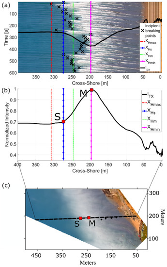
Figure 3. Breakpoint statistical location against ${\overline{I}}_{px}$. (a) Timestack image with breaking points manually detected (black crosses) and breakpoint statistical cross-shore location (colored lines). Pixel intensity ${\overline{I}}_{px}$ profile (straight black line) is superimposed on image for representation purpose, with inverted axis due to MATLAB convention. (b) Normalized ${\overline{I}}_{px}$ against the breakpoints statistical cross-shore location. S and M are shown on ${\overline{I}}_{px}$ intercepting $X_{Hs}$ and $X_{Hmin}$ locations, respectively. (c) Rectified Timex image and corresponding locations of points S and M on the transect corresponding to Timestack shown in (a). The profile of ${\overline{I}}_{px}$ shown in (a,b) is the same as the one that can be obtained by sampling the pixel intensity ($I_{TX}$) on the corresponding Timex transect (dashed black line) obtained from Timestack ${\overline{I}}_{px}$ in (c).

-

$X_{Hmax}$ as the first breaking point (farthest from the shore);

-

$X_{Hs}$ as the significant wave breaking height position, averaging the 33% of the farthest-from-shoreline breakpoints;

-

$X_{Hm}$ as the mean position among all breaking positions; and

-

$X_{Hmin}$ as the location where 100% of the waves have broken, i.e., the closest breakpoint to the shore.

To relate breakpoints statistic locations with pixel intensity variability, we computed the variation of pixel intensity along the time-axis of Timestack as the average pixel intensity profile (${\overline{I}}_{px}$), as follows:

$${\overline{I}}_{px}=\frac{1}{n}{\displaystyle \sum }_{i=1}^n{I}_{x,i}$$

(2)

where $I_{x,i}$ is the pixel intensity value and n is the number of pixels. Equivalent intensity profiles can be directly obtained by sampling the pixel intensity on Timex image (hereinafter, $I_{TX}$) over the same transect and time interval used to generate the Timestack ($I_{TX}$ = ${\overline{I}}_{px}$), as shown by Andriolo [19].

Average pixel intensity statistics ${\overline{I}}_{px}$ was coupled to the statistical fractions of breaking computed from all the breakpoints locations previously marked on Timestack (Figure 3). The blue band of the RGB image was chosen because it better represents the water color [19]. From the analysis of ${\overline{I}}_{px}$ profile, the point at which ${\overline{I}}_{px}$ starts to increase (point S) forming the typical Gaussian-like shape on breaking area (e.g., [23,28]) was found to coincide with significant wave height breaking position $X_{Hs}$. The peak of the Gausssian-like shape (point M) corresponds with the position of the most onshore breaking point $X_{Hmin}$. Finally, the ${\overline{I}}_{px}$ profile did not have any significative matching points with $X_{Hm}$ location. As we were interested in using Timex images, we focused on the use of ${\overline{I}}_{px}$ profile to spot $X_{Hs}$ and $X_{Hmin}$.

2.3. Method 1: $H{s}_{b,v}$

With the aim of finding a relationship between the ${\overline{I}}_{px}$ notable points on the profile and breaking wave height, the average bottom slope between the two breaking positions ($m_{Hs}$ = tanβ) is given by the geometrical expression (Figure 4):

$$m_{Hs}=\frac{h_{b,Hs}-h_{b,Hmin}}{L_{Hs}}$$

(3)

where $h_{b,Hs}$ and $h_{b,Hmin}$ are the water depth at $X_{Hs}$ and $X_{Hmin}$, respectively, and $L_{Hs}$ is the distance between the two positions that can be expressed, according to the analysis in Section 2.2, as:

$$L_{Hs}=X_{Hmin}-X_{Hs}=M-S$$

(4)

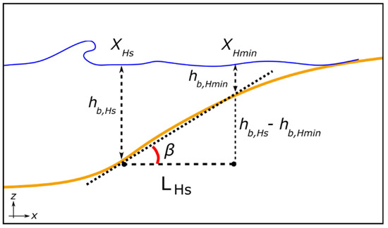
Figure 4. Empirical model sketch. The two breaking fractions $X_{Hs}$ and $X_{Hmin}$ are shown on sea surface (blue line), and β is the average beach slope (orange line) between the two positions.

At this point, Equation (3) can be written as:

$$h_{b,Hs}-h_{b,Hmin}=m_{Hs} L_{Hs}$$

(5)

At breaking point, the relation between wave height and water depth $\gamma$ (breaker index) can be expressed as [32]:

$$\frac{H_b}{h_b}=\gamma$$

(6)

where $H_b$ is the wave breaking height and $h_b$ is the water depth at the breaking point.

To simplify the model, we can divide all the members of Equation (5) by $h_{b,Hs}:$

$$\frac{h_{b,Hs}}{h_{b,Hs}}-\frac{h_{b,Hmin}}{h_{b,Hs}}=\frac{m_{Hs} L_{Hs}}{h_{b,Hs}}$$

(7)

and solve in order of $h_{b,Hs}$ as:

$$h_{b,Hs}=\frac{m_{Hs} L_{Hs}}{\left(1-\frac{h_{b,Hmin}}{h_{b,Hs}}\right)}$$

(8)

Recalling Equation (6) and using Equation (8), we obtain:

$$H{s}_{b,v}=\left(\frac{h_{b,Hs}}{h_{b,Hs}-h_{b,Hmin}}\right) m_{Hs} L_{Hs} {\gamma }_{Hs}$$

(9)

that expresses the breaking wave height $H{s}_{b,v}$ (subscript v stays for video) as proportional to the ratio between water depths at breaking locations, the local slope $m_{Hs}$, the distance between the two breakpoints $L_{Hs}$, and the non-dimensional breaker index ${\gamma }_{Hs}$.

2.4. Automated Extraction of L_Hs from Timestack and Timex

As shown in Section 2.2, the specific points which represent the limits of $L_{Hs}$ length (points M and S in Figure 3) can be extracted from the average pixel intensity ${\overline{I}}_{px}$. An automated MATLAB-based algorithm was developed to extract $L_{Hs}$ from Timestacks and from Timex images. Firstly, the algorithm was calibrated on the 94 Timestacks of Ribeira d’Ilhas, recalling that Timestacks were produced sampling a transect perpendicular to wave direction. Following Figure 5a:

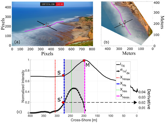
Figure 5. Automated algorithm for deriving $L_{Hs}$ from ${\overline{I}}_{px}$ and $I_{TX}$ pixel intensity profiles. (a) Oblique Timex and (b) portion of rectified Timex with detected breakline (magenta line), 10-m long portion of breakline (dashed black line), and perpendicular transect used to extract $I_{TX}$ (which correspond to ${\overline{I}}_{px}$). Red squares show points S and M found on Timex and the cyan segment is the derived $L_{Hs}$. (c) The procedure to analyze ${\overline{I}}_{px}$ and/or $I_{TX}$ profile (black line) and related first derivative (black line with triangles) to extract points S and M. Note the interception (point S’) of the first derivative of ${\overline{I}}_{px}$ (and $I_{TX}$) (line with triangles) at 0.02 with $X_{Hs}$ cross-shore position. The grey area shows the distance between S and M which corresponds to $L_{Hs}$ length.

• The peak of the Gaussian-like shape (point M) is found using a peak finder algorithm, searching for the global maximum of the Min-Max normalized ${\overline{I}}_{px}$.
• Starting from point M and moving “seaward” on ${\overline{I}}_{px}$, the point S is identified as the first point of the derivative $\frac{\partial {\overline{I}}_{px}}{\partial \mathrm{x}}$ of Min-Max normalized ${\overline{I}}_{px}$ exceeding a threshold value of 0.002, as the first derivative $\frac{\partial {\overline{I}}_{px}}{\partial \mathrm{x}}$ represents the slope of ${\overline{I}}_{px}$ at each point.

To automatically compute the right $L_{Hs}$ length directly from Timex, it is necessary to sample a transect perpendicular to wave direction. Thus, the few additional steps to be taken prior to the previously described Steps I and II are:

(i)

The breaking line is found on the whole Timex (Figure 5a,b), sampling pixel intensity of a series of parallel transect and searching the global maximum of the Min-Max normalized $I_{TX}$.

(ii)

A point is chosen along the breakline to compute the breaking height.

(iii)

A portion of the previously detected breaking line, which has the chosen point as median point, is selected. A 10-m length was considered an adequate extent to be representative of breakline portion.

(iv)

The line passing through the point, and perpendicular to the 10 m portion of breaking line is chosen as transect to sample $I_{TX}$ and therefore to find $L_{Hs}$ with Steps I and II.

The described algorithm was applied on the Timex dataset of the case study of Ribeira d’Ilhas to automatically find $L_{Hs}$, along the parameters $m_{Hs}$, $h_{b,Hs}$ and $h_{b,Hmin}$, with the aim of solving Equation (9) and thus finding $H{s}_{b,v}$.

2.5. L_Hs Versus Hydrodynamic Parameters

As a bathymetric profile is not always available, in the following, we investigate an empirical relation between the breaking wave height and the breaking pattern $L_{Hs}$ retrievable from video imagery.

The visible breakpoints locations were marked on the 94 Timestacks dataset using the manual procedure described in Section 2.2. Then, the location of $X_{Hs}$ and $X_{Hmin}$ was computed for each 10-min Timestack to find $L_{Hs}$ (Equation (4)). Each Timestack transect was coupled to the bathymetric information to retrieve the parameters required to solve Equation (9). Water depths at breaking $h_{b,Hs}$ and $h_{b,Hmin}$, along with the beach slope $m_{Hs}$, were extracted with the interpolation of the respective breakpoint statistics positions $X_{Hs}$ and $X_{Hmin}$ using the beach profile.

Solving Equation (9) also depends on breaker index $\gamma$. Numerous values of $\gamma$ are proposed in the literature [9,33] with value in the range between 0.3 and 1.6, and are based on different statistical wave heights considered, namely maximum ($H_{max}$), significant ($H_s$ or $H_{m0}$), root-mean-square ($H_{rms}$), and mean ($H_m$) wave height (e.g., see Figure 1 and Appendix in the work by Salmon et al. [34], and references therein).

In this work, we considered parameterizations of depth-induced wave breaking index proposed by McCowan [32], who found $\gamma$ = 0.78 from the solitary wave theory, referred to $H_{max}$ breaking criterion. To consider this breaker index, and also following insights from Goda [35], a solution for scaling $\gamma$ = 0.78 to $H{s}_b$ is adopted considering the ratio between wave height statistics [36]:

$$H_{0.01}=1.52 H_S$$

(10)

where $H_{0.01}$ is the height exceeded by 1% of the waves, thus a reasonable approximation to $H_{max}$ in a 10-min record. Therefore, applying the scaling factor to the breaker index $\gamma$ = 0.78:

$${\gamma }_{b,Hs}=0.78/1.52=0.51$$

(11)

To set up the method, in the following, we show the results already obtained from the manual analysis of Timestacks. Figure 6 compares the trend of $L_{Hs}$ to hydrodynamic and morphological parameters during tidal modulation. On 28 March, the $L_{Hs}$ varied between 36 m and 100 m, with a mean value of 65 m. On 29 March, $L_{Hs}$ ranged between 42 m and 170 m, with mean value of 95 m. Beach gradient $m_{Hs}$ under $L_{Hs}$ ranged from $0.005$ to $0.035$. Recalling that $m_{Hs}$ represented the average slope between $X_{Hs}$ and $X_{Hmin}$, the lowest $m_{Hs}$ value was registered on 28 March, when waves broke on the intertidal low gradient rocky platform. Highest $m_{Hs}$ value corresponded to the second day of observations, when higher waves broke seaward over a steeper profile section. The local water depth at the two considered positions had similar trend, with values between 2 and 6 m for $h_{b,Hs}$, while $h_{b,Hmin}$ was about half the value of $h_{b,Hs}$. The Iribarren number [26] varied between 0.04 and 0.48, values that can be associated to spilling wave breaking ($\xi <0.55$ [37]).

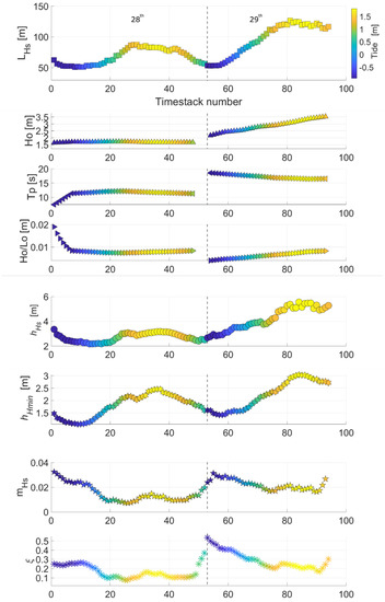
Figure 6. Wave breaking parameters derived from video imagery to solve Equation (9). $L_{Hs}$ records (squares) versus offshore significant wave height $H_o$, wave period $T_P,$ and wave steepness $H_o/L_o$ (triangles); water depth $h_{b,Hs}$ (circles) and $h_{b,Hmin}$ (hexagons); beach slope $m_{Hs}$ (pentagrams); and Iribarren number ξ (stars). Vertical black dashed line divides data from 28 March (left) and 29 March (right). The x-axis is common to all plots and indicates Timestack number (1–52 for 28 March and 53–94 for 29 March).

Overall, $L_{Hs}$ appeared to be positively correlated to offshore significant wave height, since were almost double on 29 March than on 28 March, when waves were smaller. The water depth at breaking $h_{b,Hs}$ and wave breaking pattern $L_{Hs}$ had the same trend over the dataset. The slope $m_{Hs}$ under $L_{Hs}$ changed over the time, as water level increased and breaking location moved towards the shore. The slope $m_{Hs}$ had an opposite trend of $L_{Hs}$, with steeper slope corresponding to shorter $L_{Hs}$. The slope decreased when the breakpoint locations were closer to the shoreline, since the slope gets milder. Therefore, more dissipative conditions conformed with longer $L_{Hs}$.

All above observations were supported by the computation of Pearson correlation (P), which expresses the linear correlation between $L_{Hs}$ and the several variables tested. As noted above in this section, $L_{Hs}$ was found positively correlated to $H_o$ and water depth $h_{b,Hs}$ (P = 0.86), whereas negatively correlated to beach slope (P = −0.5) and consequently to Iribarren number (P = −0.4). As the highest positive correlation was registered between $L_{Hs}$ and $h_{b,Hs}$, the direct relation between video-derived wave breaking pattern $L_{Hs}$ and hydrodynamic parameter $h_{b,Hs}$ is analyzed in the following section.

2.6. Method 2: $H{s}_{b,v24}$

Figure 7 shows direct comparisons between $L_{Hs}$ and water depth $h_{b,Hs}$ extracted at the $X_{Hs}$ over the two days, with dependence on $H_o$ and $m_{Hs}$. The best fitting value for the ratio $L_{Hs}$/$h_{b,Hs}$ was found as:

$$\frac{L_{Hs}}{h_{b,Hs}}\cong 24$$

(12)

with a R² = 0.75 and slope coefficient of 95% confidence bounds between values 23 and 25. The results suggest that the video-derived breaking pattern length $L_{Hs}$ can be related to water depth at breaking statistic location $X_{Hs}$. The relation expressed in Equation (12) does not show any particular dependence on either offshore wave height or beach slope under breaking conditions (Figure 7).

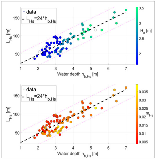
Figure 7. $L_{Hs}$ versus water depth $h_{b,Hs}$, with dependence (colors) of offshore wave height (top) and slope under breaking conditions $m_{Hs}$ (bottom). Black dashed lines indicate the best fitting y = ax. Dashed magenta lines represent upper and lower 95% prediction bounds.

The parameterization in Equation (12) is of interest in the perspective that water depth at breaking is the key parameter of wave breaking height empirical formulations (e.g., [9,33]). As the analysis suggests that the video-derived parameter $L_{Hs}$ can be used as proxy for the estimation of water depth at breaking, the simplest formulas for wave breaking height (Equation (6)) can be rewritten as:

$$\frac{H{s}_b}{L_{Hs}/24}={\gamma }_{b,Hs}$$

(13)

where $H{s}_b$ is breaking wave height at $X_{Hs}$ and ${\gamma }_{b,Hs}$ is the breaker index. We can use the value of ${\gamma }_{b,Hs}$ found from Equation (11) to finally express the video-derived breaking wave height:

$$H{s}_{b,v24}=0.51\frac{L_{Hs}}{24}$$

(14)

where the subscript v24 recalls the video-derived estimation of water depth using $L_{Hs}$.

2.7. Application at Additional Study Sites

With the aim of verifying the applicability of $H{s}_{b,v24}$ method, video images collected at four additional study sites were considered: Costa Nova, Praia Grande, Tarquinio-Paraiso, and Kourou beaches (Figure 8).

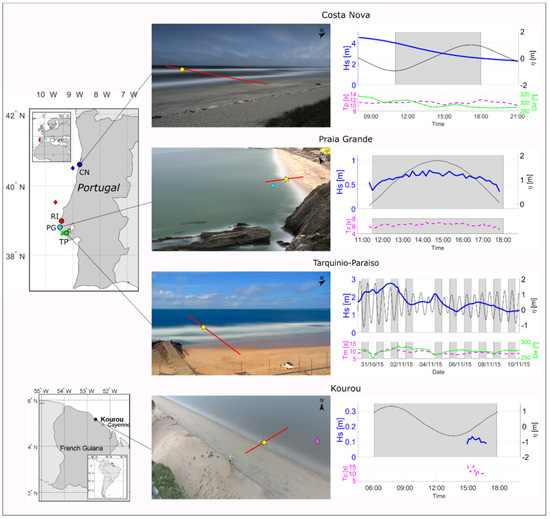
Figure 8. Four study sites for application of $H{s}_{b,v24}$ method. (left) Locations of sites, namely CN (Costa Nova), PG (Praia Grande), and TP (Tarquinio-Paraiso) in relation to RI (Ribeira d’Ilhas, development site), and KO (Kourou). (middle) Examples of oblique Timex images (central), with considered transect for sampling $I_{TX}$ and breaking location considered for the application of $H{s}_{b,v24}$ (yellow pentagram). At PG and KO, diamonds show oceanographic instrumentation deployment position. (right) Hydrodynamics during the experiences with time series of water level η, significant wave height $Hs$, wave period $T$, and wave direction Dir.

Costa Nova (40°37′05.2″N, 8°45′12.6″W) is a sandy beach located on the coastal stretch of Aveiro municipality, on the Portuguese west coast. The beach extends for about 1 km with a NE–SW orientation, limited southwards and northwards by 300 m long groins, backed by a 7-m-high dune cordon. On the crest of the dune, a temporary video system composed of an IP camera Mobotix M12 was installed on 26 November 2018 to monitor the nearshore. Offshore wave conditions were retrieved from RAIA buoy measurements (http://raia.inesctec.pt, see Figure 8 for buoy location), while the astronomical tidal constituents were used to predict the water level at the study site (http://webpages.fc.ul.pt/~cmantunes/hidrografia/hidro_mares.html).

Praia Grande (38°48′49.7″N, 9°28′38.7″W) is a headland-bay sandy beach located on a rocky coastal stretch of the Portuguese west coast, in Sintra municipality. The beach extends for about 1 km with a NE–SW orientation, limited southwards by a 50-m-high cliff above MSL, in the north by a small headland, and landward by a seawall. A field experiment was conducted at Praia Grande on 8 September 2015. An IP camera Mobotix M12 was temporary installed on the top a cliff around 50 m high, looking sideways at Praia Grande extent, and acquired video for 7 h. Hydrodynamic conditions in the shoaling and surf zone were obtained by an acoustic Doppler current profiler (ADCP) deployed during low tide.

Tarquinio-Paraiso beach (38°38′32.2″N, 9°14′21.1″W) is one of the urban beaches included in Costa da Caparica. This sandy stretch is located on the southern margin of the Tagus river inlet. The beach extends for about 400 m and it is limited sideways by groins and landward by a seawall (Figure 8). Video data were acquired by a surfcam camera placed at about 80 m above the MSL for twelve days, between 30 October 2015 and 12 November 2015. A time series of water level was obtained by the Cascais tidal gauge (38°41′30.5″N, 9°25′16.7″W), available at the web site of the Portuguese General Direction of the Territory (DGT, ftp://ftp.dgterritorio.pt/Maregrafos/Cascais). The nested application of wave propagation in Portuguese shelf, namely Water Information Forecast Framework (WIFF, ariel.lnec.pt/ [38]), was chosen as wave data source, extracted at a point located in front of Costa da Caparica (38°37′12.0″N, 9°23′24.0″W) at 50 m depth.

Kourou beach (5°10′38.4″N, 52°38′49.6″W) is a sandy open beach located on the French Guyanese coast, about 60 km northwest from capital Cayenne. A shore-based video monitoring station was implemented in French Guyana in late November 2017. The optical system was composed by an Axis IP camera installed on a 10-m-high aluminum tower that was deployed in proximity of the beach. A field experiment was conducted at Kourou on 7 December 2017. A PT was deployed at a depth of 1 m above MSL for measuring water level timeseries and computing significant wave height for 2 h.

Images collected at all the sites were rectified at the corresponding water level with Cosmos software [25], in combination with C-Pro tool [39] in case of surfcam source. The 10-min rectified Timex images were produced from video sequences and automatically processed to sample a single cross-shore $I_{TX}$ profile. The $I_{TX}$ dataset was processed by the algorithm described in Section 2.4 to find $L_{Hs}$. Table 1 presents the (available) morphology, the hydrodynamic characteristics during the field experiences, along with video dataset properties of each site considered in applying $H{s}_{b,v24}$ method.

Table 1. Video system, beach characteristics, and wave conditions observed during the experiments for each study site, namely CN (Costa Nova), PG (Praia Grande), TP (Tarquinio-Paraiso), KO (Kourou), and RI (Ribeira d’Ilhas, development site).

Site	Video Source	Image Resolution	Dataset (No. Timex)	Wave Height Range (m)	Beach Bottom	Breaking Zone	Wave Data Source
CN	video station	2048 × 1536	36	2.57 ± 3.75	sandy	outer bar	Offshore Buoy
PG	video station	2048 × 1536	49	0.46 ± 0.85	sandy	shore	ADCP
TP	surfcam	800 × 450	655	1.17 ± 2.76	sandy	outer bar	model (WIFF)
KO	video station	1920 × 1080	70	0.08 ± 0.13	sandy	shore	PT
RI	surfcam	800 × 450	92	1.04 ± 3.27	rocky	shore	model (SWASH)

Overall, the whole dataset consisted in 902 Timex images. Hydrodynamics conditions ranged from low to high energetic wave conditions (H₀ from 0.1 m to 3.8 m). As is clear by the Timex images in Figure 8, Costa Nova and Tarquinio-Paraiso beaches are barred beaches; therefore, we computed the breaking wave height at the (first) seaward breaking pattern on Timex. At Praia Grande and Kourou beaches, waves were breaking near the shore. The dataset of the case study (Ribeira d’Ilhas, Section 2.1) is also included in Table 1 for a comprehensive presentation.

3. Results

3.1. Automated Algorithm and Numerical Model

A first stage focused on the evaluation of breakpoint statistical locations extracted from Timex at Ribeira d’Ilhas case study (Figure 9). All breaking points were manually marked on Timestack dataset and $X_{Hs}$ and $X_{Hmin}$ computed as in Section 2.2. The same breakpoint location statistics $X_{Hs}$ and $X_{Hmin}$ were extracted at each Timex over the transect used to produce Timestacks, by the algorithm described in Section 2.4.

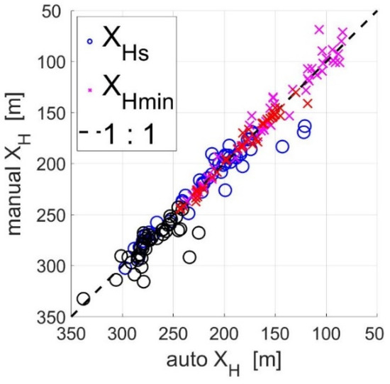
Figure 9. Comparison between $X_{Hs}$ and $X_{Hmin}$ found from manual analysis of Timestacks, and automatically derived from ${\overline{I}}_{px}$. Circles represent $X_{Hs}$ (blue and black from 28 and 29 March, respectively), crosses to $X_{Hmin}$ (magenta and red from 28 and 29 March, respectively).

For both points, namely $X_{Hs}$ and $X_{Hmin}$, the agreement between manually- and automatically-retrieved locations was close to identity on both days (Figure 9). Using automatically-retrieved $X_{Hs}$ and $X_{Hmin}$, the whole parameters necessary to solve Equation (9), thus to retrieve $H{s}_{b,v}$ were found using two-days dataset. For each 10-min Timex, the distance $L_{Hs}$ was found as the distance between the automatically-retrieved $X_{Hs}$ and $X_{Hmin}$ (Equation (3)). The beach gradient $m_{Hs}$ was computed as the average beach profile slope between the cross-shore boundaries of $L_{Hs}$, while $h_{b,Hs}$ and $h_{b,Hmin}$ were the actual water levels at each $X_{Hs}$ and $X_{Hmin}$ locations.

The second stage aimed to verify the accuracy of SWASH model. A good agreement was found between the simulated and the measured Hs over the tidal cycle for both days (Figure 10). The differences between the measured and the simulated Hs assessed with root mean square error (RMSE) varied between 0.08 and 0.13 m, with the best performance on 28 March. Significant wave height was slightly underestimated by the model during the more energetic second day. Overall, the normalized RMSE (NRMSE) values were between 9% and 13% during the two days. These results confirm that the numerical solution obtained by SWASH can be used to assess the accuracy of the proposed video-based methods.

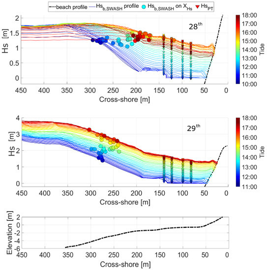
Figure 10. SWASH model results for the two days. Circles show the $H{s}_{b,SWASH}$ extracted at $X_{Hs}$, which were found from video data at the corresponding time interval. Triangles show $Hs$ measured by PTs at their cross-shore locations. The legend at the top is common both graphs. The related beach profile transect is shown at the bottom of the figure.

3.2. Wave Breaking Height Assessment

Using the records of the automatically video-derived parameters, Figure 11 shows the video-derived breaking wave height computed using the two proposed $H{s}_{b,v}$ and $H{s}_{b,v24}$ methods for the 94 Timex, compared with numerical models results $H{s}_{b,SWASH}$ extracted at the video-derived $X_{Hs}$ locations.

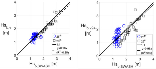
Figure 11. Video-derived breaking wave height from the two methods, namely $H{s}_{b,v}$ (left) and the $H{s}_{b,v24}$ (right) against SWASH model results. Thick black lines indicate identity, while dashed black lines represent the best fitting.

Considering $H{s}_{b,v}$ (Equation (9)) and the target values obtained by SWASH model, $H{s}_{b,v}$ method returned a satisfactory estimation, with a RMSE of about 0.2 m for both days (Table 2). Higher waves were slightly underestimated during the second day, suggesting that a higher value of the breaker index ${\gamma }_{b,Hs}$ might be more appropriated in case of a steeper $m_{Hs}$.

Table 2. Detailed video-derived results from $H{s}_{b,v}$ and $H{s}_{b,v24}$.

		28 March	29 March	Dataset
Ho	min ± max	1.64 ± 1.72	2.16 ± 3.53	1.64 ± 3.53
Hsb_SWASH	min ± max	1.04 ± 1.82	1.39 ± 3.27	1.04 ± 3.27
records		52	42	94
Hsb_v	Bias	0.02	−0.12	−0.04
	RMSE	0.19	0.22	0.21
	NRMSE	14%	12%	9%
Hsb_v24	Bias	0.17	−0.28	−0.03
	RMSE	0.55	0.43	0.5
	NRMSE	38%	23%	22%

The results obtained by the $H{s}_{b,v24}$ method (Equation (14)) were more scattered around the identity line, especially for breaking wave height under 2 m (Figure 11). In fact, the highest RMSE was registered during the first day, when wave conditions were constant and less energetic than the second day. Nevertheless, considering the whole dataset, NRMSE was about 22% for a range of modeled breaking wave height comprised between 1 and 3.3 m (Table 2). Although the NRMSE of $H{s}_{b,v}$ (9%) was about half of the one obtained by $H{s}_{b,v24}$, $H{s}_{b,v24}$ results are reasonable considering that they were derived exclusively from video without any other additional data.

A last computation was pursed to search for a constant value of the breaker index ${\gamma }_{b,Hs}$ imposing the identity between $H{s}_{b,v24}$ records and $H{s}_{b,SWASH}$ dataset. It was found that the best fitting value of ${\gamma }_{b,Hs}$ was 0.54, which improved the accuracy to an RMSE = 0.42 m when applied on the dataset. The same value of best fitting ${\gamma }_{b,Hs}$ = 0.54 was found for $H{s}_{b,v}$ against $H{s}_{b,SWASH}$; however, when such value was used to solve Equation (9), it did not ameliorate significantly the results that were obtained with ${\gamma }_{b,Hs}$ = 0.51.

3.3. Application at Additional Study Sites

Figure 12 shows the breaking wave height computed with $H{s}_{b,v24}$ method in comparison with the wave data sources, applied on Timex images produced from video collected at the four additional sites together with the one from the development site. Despite the diverse video devices, the different hydrodynamic conditions and the variable wave data sources used for comparison breaking wave height were assessed with fair accuracy at all study sites when compared to the typical wave sources (Table 3).

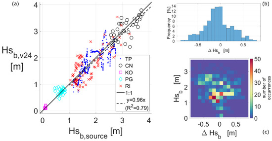
Figure 12. Results of $H{s}_{b,v24}$. (a) Scatter plot of results obtained at all the five considered field sites namely. TP (Tarquinio-Paraiso), CN (Costa Nova), KO (Kourou), PG (Praia Grande), and RI (Ribeira d’Ilhas). Thick black line indicates identity, while the dashed black line indicates the best fit (reported in legend). (b) Cumulative histogram and (c) 2D histogram of ∆$H{s}_b$ ($H{s}_{b,v24}$ − $H{s}_{b,source}$).

Table 3. Details of $H{s}_{b,v24}$ results, coupled to video device, morphological characteristics, and wave data source for each considered site, namely CN (Costa Nova), PG (Praia Grande), TP (Tarquinio-Paraiso), KO (Kourou), and RI (Ribeira d’Ilhas, development site).

Site	Video Source	Dataset (No. Timex)	Wave Height Range (m)	Beach Sediment	Breaking Zone	Wave Data Source for Comparison	RMSE (m)	NRMSE (%)
CN	video station	36	2.57 ± 3.75	sandy	outer bar	Offshore buoy	0.3	10%
PG	video station	49	0.46 ± 0.85	sandy	shore	ADCP	0.12	18%
TP	surfcam	655	1.17 ± 2.76	sandy	outer bar	model (WIFF)	0.35	21%
KO	video station	70	0.08 ± 0.13	sandy	shore	PT	0.02	20%
RI	surfcam	92	1.04 ± 3.27	rocky	shore	model (SWASH)	0.5	22%

At Costa Nova and at Tarquinio-Paraiso beaches, $H{s}_{b,v24}$ was computed considering the breaking over the outer bar, with a final RMSE close to 0.3 m for significant wave height between 1 and 4 m. The best NRMSE was achieved at Costa Nova, where offshore buoy measurements were used for comparison (Table 3). On the other hand, the results obtained with the longest dataset at Tarquinio-Paraiso (10 days of continuous observations) proved the suitability of $H{s}_{b,v24}$ method for long-term estimation of breaking wave height, returning a correlation coefficient of 0.80 with Wiff model. At Kourou and Praia Grande beaches, breaking wave height on the shore was lower than 1 m. When compared against oceanographic instrumentation measurements (PT and ADCP, respectively), $H{s}_{b,v24}$ returned a NRMSE similar to the sites with more energetic waves and with breaking over the outer bar.

4. Discussion

4.1. Video-Based Methods

The two proposed methods to measure breaking wave height from video imagery showed several advantages over the existing techniques based on optical images. Firstly, they do not require sophisticated image processing techniques (e.g., [18]), making their application easier to replicate. Secondly, they allow the estimation of the breaking wave height with the use of a commonly produced Timex images, whereas previous methodologies are merely Timestack-based [17,18]. In fact, Timex images have been operatively and routinely produced from all existing Argus stations and coastal video systems worldwide over the last 30 years. The use of Timex is opportunistic also because it allows sampling multiple arrays of transects over alongshore domain, hence characterizing breaking wave height over the whole monitored area, without the need of producing a Timestack image for each transect of interest. Finally, both methods can be directly coupled to the numerous applications that use Timex properties for studying coastal processes [14,16,40,41].

A first limitation of both methods is related with the video sampling time interval used, as the methods are based on 10-min Timex. Although this is a standard interval used, further investigation should be addressed if the methods are to be applied on images produced with different time sampling. In addition, the methods return significant breaking wave height averaged within 10 min, whereas existing video-derived measurements [17,18] allow wave-by-wave breaking height analysis.

The wave breaking pattern ($L_{Hs}$) detection should also be discussed. It is fundamental to sample on Timex a transect perpendicular to the main high intensity breaking pattern for a correct extraction of $L_{Hs}$ length (Figure 5b,c). The second limitation for both methods regards this aspect, due to the fact that, while regular incipient and breaking dissipation lines could be easy to detect, a wide inner surf area with highly irregular breaking patterns might cause difficulties in the detections of $X_{Hs}$ and $X_{Hmin}$, thus misleading the evaluation of $L_{Hs}$ length. This is particularly true, for instance, when rip currents are present in the surf zone, due the fact that averaged breaking patterns over 10-min are not clear and uniform (e.g., [42]).

4.2. Breaker Index

The choice of the breaking index value ${\gamma }_b$ is a source of uncertainty for both methods. The extensive state-of-the-art (e.g., [9,33,43]) shows that ${\gamma }_b$ can be expressed as a constant value, or as a function of offshore wave properties and beach slope. Therefore, the selection of the optimal formulation and/or the right estimation of ${\gamma }_b$ is not an easy task. The easiest solution adopted in this work, ${\gamma }_{b,Hs}$ = 0.51, was based on the rational choice that a constant value allowed to use the same breaker index for both the presented methods, emphasizing that the second method intends to provide a tool for estimating breaking wave height merely from video, independently on wave conditions and when field data (bathymetry and beach slope) are not available.

Overall, the ${\gamma }_{b,Hs}$ constant value solution led to satisfactory results for the wide range of $H{s}_b$ values considered, when applied on the presented field sites dataset. Nevertheless, future work might contemplate the parameterization of the best breaker index to be used, also taking in account that we found ${\gamma }_{b,Hs}$ = 0.54 as best fitting value for mild beach slope ranging between 0.005 and 0.035 at the case study, which, however, did not improve significantly the results (Section 3.2). Further developments should also consider the influence of wave reflection on breaker index value, as it was found that for irregular waves ${\gamma }_b$ value can be influenced up to 15% by reflected waves [13].

4.3. Method 1: $H{s}_{b,v}$

When bathymetry is available, the use of $H{s}_{b,v}$ method may be a good alternative to the development of a more computationally-demanding numerical wave model. On the other hand, the requirement for the beach topo-bathymetry limits the application of $H{s}_{b,v}$, since a nearshore bottom profile survey is a difficult task to perform, especially at high energy environments. Where direct measurements are missing, video monitoring has been shown to be a valuable method to estimate nearshore bathymetry [29,44,45] and/or beach intertidal topography [46,47,48]. Therefore, a combined use of video methodologies may supply the water depth information required for the solution of the empirical model. Similar formulations for $H{s}_{b,v}$ available in the literature have also been tested (e.g., [49]) and lead to similar empirical relations; however, Equation (9) was built on geometrical relationships of hydrodynamic parameters and thus was preferred to others.

4.4. Method 2: $H{s}_{b,v24}$

$H{s}_{b,v24}$ has much potential for remotely estimating breaking wave height merely from video imagery, without the need of additional data (Equation (14)). In fact, the fairly small differences in $H{s}_b$ between the remote sensing technique results and the different sources (Table 3, average NMRES of 18%) suggest the technique as a valid tool for wave characterization in the nearshore, in particular for long-term monitoring. Further studies should focus on a better physical understanding of $L_{Hs}$ dependence on beach slope, since surf zone width has a dependency on the bottom slope (e.g., [49]). The lack of topo-bathymetric data did not allow this analysis; however, the number of sites considered, the variability of breaking zones, and the location of the outer surf zone during different tidal levels may suggest that the method can be applied over a wide variety of bottom configurations.

Further development of the method may also account for the influence of wave reflection on ${\gamma }_{b,Hs}$, in particular under reflective conditions, although it was previously shown that wave reflection does not seem to influence the location of the breakpoint [13] and hence may not affect (time-averaged) $L_{Hs}$ length.

The use of the fraction of wave breaking pattern $L_{Hs}/24$ assessed overall good results at all five sites, although it is worth noting that at the case study beach slope ranged between 0.005 and 0.035, and topography measurements were not available at the additional four sites. In this perspective, progresses about the hydrodynamic properties and dependences of $L_{Hs}$ may be investigated, for instance, by LiDAR technique, which can provide high resolution data of wave transformation [50,51] and easily coupled to video [47].

It is worth mentioning that, since the ratio $L_{Hs}/24$ can be used to approximate the local water depth at breaking, the possibility of using such relation for a rough estimation of beach profile under breaking conditions from Timex images could also be explored. As final suggestion, further work may investigate the potential of the method being applied to snapshots [52], to UAS images (e.g., [53,54,55]) and/or to surfcam images [14,56,57] for a quasi-real time estimation of breaking wave height.

5. Conclusions

This work presents two video-based methods to estimate breaking wave height from Timex, which are images universally produced by coastal video monitoring systems worldwide. Both methods were developed and applied with images acquired in the field from shore-based video monitoring stations.

The pixel intensity variation over a pixel transect sampled on Timex was related to breaking wave fractions, hence exploited to spot the location of specific breakpoints with the final aim of computing a video-derived parameter associated with surf zone length, namely $L_{Hs}$. The first method ($H{s}_{b,v}$) couples $L_{Hs}$ to the available bathymetric data, while the second method ($H{s}_{b,v24}$) proposes the relationship $L_{Hs}/24$ for approximating the local water depth and thus to retrieve breaking wave height merely from video. A good agreement was found between the modeled wave data at a field case study for both the methods, where $H{s}_{b,v}$ has double the rate of precision, namely a NRMSE of 9%, with respect to $H{s}_{b,v24}$. Nevertheless, the potential of $H{s}_{b,v24}$ as remote tool for breaking wave height estimation was demonstrated when the method was applied at four additional sites, where bathymetric data were not available, returning an average NRMSE of 18% for around 900 records.

Both methods can be easily implemented as a cost-effective tool in the operative coastal video systems worldwide and have the potentiality to be applied to the existing dataset and/or coupled to the numerous other Timex applications.

References

- Bird, E.C.F. Coastal Geomorphology: An Introduction; John Wiley & Sons: Chichester, UK, 2014. [Google Scholar]
- Meer, J.W.V.D.; Stam, C.J.M. Wave Runup on Smooth and Rock Slopes of Coastal Structures. J. Waterway Port Coast. Ocean Eng. 1992, 118, 534–550. [Google Scholar] [CrossRef]
- Ferreira, Ó.; Ciavola, P.; Armaroli, C.; Balouin, Y.; Benavente, J.; Del Río, L.; Deserti, M.; Esteves, L.S.; Furmanczyk, K.; Haerens, P.; et al. Coastal storm risk assessment in Europe: Examples from 9 study sites. J. Coast. Res. 2009, SI56, 1632–1636. [Google Scholar]
- Svendsen, I.A. Introduction to Nearshore Hydrodynamics; World Scientific: Hackensack, NJ, USA, 2006. [Google Scholar]
- Battjes, J.A. Surf Similarity. In Proceedings of the 14th Asce Coastal Engineering Conference, Copenhagen, Denmark, 24–28 June 1974; Volume 1, pp. 466–480. [Google Scholar]
- Battjes, J.A. Surf-Zone Dynamics. Annu. Rev. Fluid Mech. 1988, 20, 257–291. [Google Scholar] [CrossRef]
- Booij, N.; Ris, R.C.; Holthuijsen, L.H. A third-generation wave model for coastal regions 1. Model description and validation. J. Geophys. Res. Ocean. 1999, 104, 7649–7666. [Google Scholar] [CrossRef]
- Zijlema, M.; Stelling, G.; Smit, P. SWASH: An operational public domain code for simulating wave fields and rapidly varied flows in coastal waters. Coast. Eng. 2011, 58, 992–1012. [Google Scholar] [CrossRef]
- Camenen, B.; Larson, M. Predictive Formulas for Breaker Depth Index and Breaker Type. J. Coast. Res. 2007, 234, 1028–1041. [Google Scholar] [CrossRef]
- Robertson, B.; Hall, K.; Zytner, R.; Nistor, I. Breaking Waves: Review of Characteristic Relationships. Coast. Eng. J. 2013, 55, 1350002. [Google Scholar] [CrossRef]
- Browne, M.; Castelle, B.; Strauss, D.; Tomlinson, R.; Blumenstein, M.; Lane, C. Near-shore swell estimation from a global wind-wave model: Spectral process, linear, and artificial neural network models. Coast. Eng. 2007, 54, 445–460. [Google Scholar] [CrossRef]
- Sutherland, P.; Melville, W.K. Field measurements and scaling of ocean surface wave-breaking statistics. Geophys. Res. Lett. 2013, 40, 3074–3079. [Google Scholar] [CrossRef]
- Martins, K.; Blenkinsopp, C.E.; Almar, R.; Zang, J. The influence of swash-based reflection on surf zone hydrodynamics: a wave-by-wave approach. Coast. Eng. 2017, 122, 27–43. [Google Scholar] [CrossRef]
- Andriolo, U.; Sánchez-García, E.; Taborda, R. Operational use of surfcam online streaming images for coastal morphodynamic studies. Remote Sens. 2019, 11, 78. [Google Scholar] [CrossRef]
- Harley, M.D.; Andriolo, U.; Armaroli, C.; Ciavola, P. Shoreline rotation and response to nourishment of a gravel embayed beach using a low-cost video monitoring technique: San Michele-Sassi Neri, Central Italy. J. Coast. Conserv. 2014, 18, 551–565. [Google Scholar] [CrossRef]
- Holman, R.A.; Stanley, J. The history and technical capabilities of Argus. Coast. Eng. 2007, 54, 477–491. [Google Scholar] [CrossRef]
- Almar, R.; Cienfuegos, R.; Catalán, P.A.; Michallet, H.; Castelle, B.; Bonneton, P.; Marieu, V. A new breaking wave height direct estimator from video imagery. Coast. Eng. 2012, 61, 42–48. [Google Scholar] [CrossRef]
- Gal, Y.; Browne, M.; Lane, C. Automatic estimation of nearshore wave height from video timestacks. In Proceedings of the 2011 International Conference on Digital Image Computing: Techniques and Applications (DICTA 2011), Noosa, Australia, 6–8 December 2011; pp. 364–369. [Google Scholar]
- Andriolo, U. Nearshore Wave Transformation Domains from Video Imagery. J. Mar. Sci. Eng. 2019, 7, 186. [Google Scholar] [CrossRef]
- Shand, T.; Bailey, D.; Shand, R. Automated Detection of Breaking Wave Height Using an Optical Technique. J. Coast. Res. 2012, 28, 671–682. [Google Scholar]
- Huntley, D.; Saulter, A.; Kingston, K.; Holman, R. Use of video imagery to test model predictions of surf heights. WIT Trans. Ecol. Environ. 2009, 126, 39–50. [Google Scholar]
- Armaroli, C.; Ciavola, P. Dynamics of a nearshore bar system in the northern Adriatic: A video-based morphological classification. Geomorphology 2011, 126, 201–216. [Google Scholar] [CrossRef]
- Turner, I.L.; Whyte, D.; Ruessink, B.G.; Ranasinghe, R. Observations of rip spacing, persistence and mobility at a long, straight coastline. Mar. Geol. 2007, 236, 209–221. [Google Scholar] [CrossRef]
- Antunes, C.; Taborda, R. Sea level at cascais tide gauge: Data, analysis and results. J. Coast. Res. 2009, 56, 218–222. [Google Scholar]
- Taborda, R.; Silva, A. COSMOS: A lightweight coastal video monitoring system. Comput. Geosci. 2012, 49, 248–255. [Google Scholar] [CrossRef]
- Holthuijsen, L.H. Waves in Oceanic and Coastal Waters; Cambridge University Press: Cambridge, UK, 2015. [Google Scholar]
- Battjes, J.A.; Janssen, J.P.F.M. Energy Loss and Set-Up Due To Breaking of Random Waves. In Proceedings of the 16th International Conference on Coastal Engineering, Hamburg, Germany, 27 August–3 September 1978; Volume 1, pp. 569–587. [Google Scholar]
- Lippmann, T.C.; Holman, R.A. Quantification of sand bar morphology: a video technique based on wave dissipation. J. Geophys. Res. 1989, 94, 995–1011. [Google Scholar] [CrossRef]
- Catálan, P.A.; Haller, M.C. Remote sensing of breaking wave phase speeds with application to non-linear depth inversions. Coast. Eng. 2008, 55, 93–111. [Google Scholar] [CrossRef]
- Haller, M.C.; Catalán, P.A. Remote sensing of wave roller lengths in the laboratory. J. Geophys. Res. Ocean. 2009, 114. [Google Scholar] [CrossRef]
- Kamphuis, J.W. Introduction to Coastal Engineering and Management; World Scientific: Hackensack, NJ, USA, 2012. [Google Scholar]
- McCowan, J. On the highest wave of permanent type. Philos. Mag. J. Sci. 1894, 5, 351–358. [Google Scholar] [CrossRef]
- Robertson, B.; Nistor, I.; Hall, K.; Buckham, B. Remote measurement and prediction of breaking wave parameters. Coast. Eng. Proc. 2014, 1, 41. [Google Scholar] [CrossRef]
- Salmon, J.E.; Holthuijsen, L.H.; Zijlema, M.; van Vledder, G.P.; Pietrzak, J.D. Scaling depth-induced wave-breaking in two-dimensional spectral wave models. Ocean Model. 2015, 87, 30–47. [Google Scholar] [CrossRef]
- Goda, Y. Reanalysis of regular and random breaking wave statistics. Coast. Eng. J. 2010, 52, 71–106. [Google Scholar] [CrossRef]
- Kamphuis, J.W. Incipient wave breaking. Coast. Eng. 1991, 15, 185–203. [Google Scholar] [CrossRef]
- Gaughan, M.K.; Komar, P.D. The theory of wave propagation in water of gradually varying depth and the prediction of breaker type and height. J. Geophys. Res. 1975, 80, 2991–2996. [Google Scholar] [CrossRef]
- Fortunato, A.B.; Oliveira, A.; Rogeiro, J.; Tavares da Costa, R.; Gomes, J.L.; Li, K.; de Jesus, G.; Freire, P.; Rilo, A.; Mendes, A.; et al. Operational forecast framework applied to extreme sea levels at regional and local scales. J. Oper. Oceanogr. 2017, 10, 1–15. [Google Scholar] [CrossRef]
- Sánchez-García, E.; Balaguer-Beser, A.; Pardo-Pascual, J.E. C-Pro: A coastal projector monitoring system using terrestrial photogrammetry with a geometric horizon constraint. ISPRS J. Photogramm. Remote Sens. 2017, 128, 255–273. [Google Scholar] [CrossRef]
- Román-Rivera, M.A.; Ellis, J.T. A synthetic review of remote sensing applications to detect nearshore bars. Mar. Geol. 2019, 408, 144–153. [Google Scholar] [CrossRef]
- Splinter, K.D.; Harley, M.D.; Turner, I.L. Remote sensing is changing our view of the coast: Insights from 40 years of monitoring at Narrabeen-Collaroy, Australias. Remote Sens. 2018, 10, 1744. [Google Scholar] [CrossRef]
- Moura, T.; Baldock, T.E. Remote sensing of the correlation between breakpoint oscillations and infragravity waves in the surf and swash zone. J. Geophys. Res. Ocean. 2017, 122, 3106–3122. [Google Scholar] [CrossRef]
- Robertson, B.; Gharabaghi, B.; Hall, K. Prediction of Incipient Breaking Wave Heights Using Artificial Neural Networks and Empirical Relationships. Coast. Eng. J. 2015, 31, 150901234203000. [Google Scholar] [CrossRef]
- Holman, R.; Plant, N.; Holland, T. CBathy: A robust algorithm for estimating nearshore bathymetry. J. Geophys. Res. Ocean. 2013, 118, 2595–2609. [Google Scholar] [CrossRef]
- Almar, R.; Cienfuegos, R.; Catalán, P.A.; Birrien, F.; Castelle, B.; Michallet, H. Nearshore bathymetric inversion from video using a fully non-linear Boussinesq wave model. J. Coast. Res. 2011, 64, 3–7. [Google Scholar]
- Vousdoukas, M.I.; Ferreira, P.M.; Almeida, L.P.; Dodet, G.; Psaros, F.; Andriolo, U.; Taborda, R.; Silva, A.N.; Ruano, A.; Ferreira, Ó.M. Performance of intertidal topography video monitoring of a meso-tidal reflective beach in South Portugal. Ocean Dyn. 2011, 61, 1521–1540. [Google Scholar] [CrossRef]
- Andriolo, U.; Almeida, L.P.; Almar, R. Coupling terrestrial LiDAR and video imagery to perform 3D intertidal beach topography. Coast. Eng. 2018, 140, 232–239. [Google Scholar] [CrossRef]
- van Dongeren, A.; Plant, N.; Cohen, A.; Roelvink, D.; Haller, M.C.; Catalán, P. Beach Wizard: Nearshore bathymetry estimation through assimilation of model computations and remote observations. Coast. Eng. 2008, 55, 1016–1027. [Google Scholar] [CrossRef]
- Thornton, E.B.; Guza, R.T. Energy saturation and phase speeds measured on the natural beach. J. Geophys. Res. 1982, 87, 9499–9508. [Google Scholar] [CrossRef]
- Martins, K.; Blenkinsopp, C.E.; Zang, J. Monitoring individual wave characteristics in the inner surf with a 2-dimensional laser scanner (LiDAR). J. Sens. 2016, 2016, 7965431. [Google Scholar] [CrossRef]
- Martins, K.; Blenkinsopp, C.E.; Power, H.E.; Bruder, B.; Puleo, J.A.; Bergsma, E.W.J. High-resolution monitoring of wave transformation in the surf zone using a LiDAR scanner array. Coast. Eng. 2017, 128, 37–43. [Google Scholar] [CrossRef]
- Harley, M.D.; Kinsela, M.A.; Sánchez-García, E.; Vos, K. Shoreline change mapping using crowd-sourced smartphone images. Coast. Eng. 2019, 150, 175–189. [Google Scholar] [CrossRef]
- Holman, R.A.; Brodie, K.L.; Spore, N.J. Surf Zone Characterization Using a Small Quadcopter: Technical Issues and Procedures. IEEE Trans. Geosci. Remote Sens. 2017, 55, 2017–2027. [Google Scholar] [CrossRef]
- Gonçalves, G.R.; Pérez, J.A.; Duarte, J. Accuracy and effectiveness of low cost UASs and open source photogrammetric software for foredunes mapping. Int. J. Remote Sens. 2018, 39, 5059–5077. [Google Scholar] [CrossRef]
- Bergsma, E.W.J.; Almar, R.; Melo de Almeida, L.P.; Sall, M. On the operational use of UAVs for video-derived bathymetry. Coast. Eng. 2019, 152, 103527. [Google Scholar] [CrossRef]
- Mole, M.A.; Mortlock, T.R.C.; Turner, I.L.; Goodwin, I.D.; Splinter, K.D.; Short, A.D. Capitalizing on the surfcam phenomenon: a pilot study in regional-scale shoreline and inshore wave monitoring utilizing existing camera infrastructure. J. Coast. Res. 2013, 165, 1433–1438. [Google Scholar] [CrossRef]
- Bracs, M.A.; Turner, I.L.; Splinter, K.D.; Short, A.D.; Lane, C.; Davidson, M.A.; Goodwin, I.D.; Pritchard, T.; Cameron, D. Evaluation of Opportunistic Shoreline Monitoring Capability Utilizing Existing “Surfcam” Infrastructure. J. Coast. Res. 2016, 319, 542–554. [Google Scholar] [CrossRef]
© 2020 by the authors. Licensee MDPI, Basel, Switzerland. This article is an open access article distributed under the terms and conditions of the Creative Commons Attribution (CC BY) license (http://creativecommons.org/licenses/by/4.0/).