Article

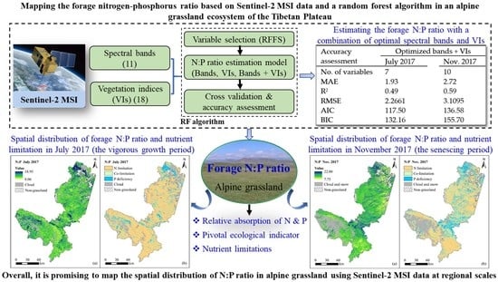
Mapping the Forage Nitrogen-Phosphorus Ratio Based on Sentinel-2 MSI Data and a Random Forest Algorithm in an Alpine Grassland Ecosystem of the Tibetan Plateau

State Key Laboratory of Grassland Agro-Ecosystems, Key Laboratory of Grassland Livestock Industry Innovation, Ministry of Agriculture and Rural Affairs, Engineering Research Center of Grassland Industry, Ministry of Education, College of Pastoral Agriculture Science and Technology, Lanzhou University, Lanzhou 730000, China
*
Author to whom correspondence should be addressed.
Remote Sens. 2020, 12(18), 2929; https://doi.org/10.3390/rs12182929
Submission received: 6 August 2020 / Revised: 6 September 2020 / Accepted: 7 September 2020 / Published: 10 September 2020
(This article belongs to the Collection Sentinel-2: Science and Applications)

Abstract

:
Nondestructive and accurate estimating of the forage nitrogen–phosphorus (N:P) ratio is conducive to the real-time diagnosis of nutrient limitation and the formulation of a management scheme during the growth and development of forage. New-generation high-resolution remote sensors equipped with strategic red-edge wavebands offer opportunities and challenges for estimating and mapping forage N:P ratio in support of the sustainable utilization of alpine grassland resources. This study aims to detect the forage N:P ratio as an ecological indicator of grassland nutrient content by employing Sentinel-2 multispectral instrument (MSI) data and a random forest (RF) algorithm. The results showed that the estimation accuracy (R2) of the forage N:P ratio model established by combining the optimized spectral bands and vegetation indices (VIs) is 0.49 and 0.59 in the vigorous growth period (July) and the senescing period (November) of forage, respectively. Moreover, Sentinel-2 MSI B9 and B12 bands contributed greatly to the estimation of the forage N:P ratio, and the VIs (RECI2) constructed by B5 and B8A bands performed well in the estimation of the forage N:P ratio. Overall, it is promising to map the spatial distribution of the forage N:P ratio in alpine grassland using Sentinel-2 MSI data at regional scales. This study will be potentially beneficial in implementing precise positioning of vegetation nutrient deficiency and scientific fertilization management of grassland.

Graphical Abstract

1. Introduction

The biochemical parameters of forage in natural alpine grasslands, such as nitrogen (N), phosphorus (P) and chlorophyll, are important aspects of forage nutrition conditions and feed value and play an important role in the life cycle of plants [1,2]. As an essential component of protein, N promotes the development and formation of stems, leaves and fruits and therefore is a crucial nutrient element affecting grassland biomass [3,4]. P promotes the metabolism of individual plants and is an essential nutrient for grassland plants living in the harsh environment of the Tibetan Plateau [5,6]. The plant nitrogen–phosphorus (N:P) ratio is a pivotal ecological indicator representing the relative absorption of N and P that can reflect the growth status of vegetation [7,8,9].
Despite considerable research [7,10,11], a critical value for the N:P ratio of forage is still not a unified standard in different ecosystems. Overall, the division scheme of threshold developed by Tessier and Raynal can be applied to natural alpine grassland ecosystems [10]. In this scheme, an N:P ratio < 14 is likely plant N limitation, an N:P ratio > 16 tends to indicate P deficiency, and an N:P ratio ranging from 14 to 16 indicates that the growth of vegetation is limited by both N and P [10]. The N:P ratio not only is related to species richness, functional traits and productivity but also indicates potential limitations of N and P [12,13]. Therefore, investigating the spatial distribution characteristics of the N:P ratio at a regional scale can provide useful information for the rational utilization of alpine grassland resources and the diagnosis of forage growth status.
Remote sensing technology has provided a more convenient and efficient approach for the dynamic monitoring of grassland vegetation at the landscape and regional scales [14,15]. The methods of estimating forage biochemical parameters can be mainly divided into two types, viz. the physically based method and empirical method [16]. Radiative transfer models (RTMs) explain the interaction of solar radiation in plant leaves according to the optical laws, thus offer many advantages in the generalizability and robustness. The empirical method offers a preliminary understanding of the relationship between forage biochemical parameters and spectral variables (i.e., spectral features and vegetation indices (VIs)), and is relatively easy to perform [17]. Studies on the estimation of forage N content and spatial inversion based on multisource high-resolution spectral data have become increasingly mature. Forage N have been shown to correlate strongly with chlorophyll [18]. The detection of forage N using remote sensing technology is generally associated with the absorption of chlorophyll, and usually includes the spectral regions related to chlorophyll detection (i.e., the red-edge and near-infrared (NIR) regions). N is involved in the protein synthesis, which facilitate the photosynthetic process [19]. The red-edge position is the point where the vegetation reflectance spectrum has the maximum slope in the 680–750 nm [20]. Studies have indicated that the red-edge is less sensitive to atmospheric effects and soil background. The red-edge position has been extensively applied in estimating leaf area index, N, chlorophyll and biomass [21,22]. However, due to the few identifiable spectral absorption features and low content of P in grassland plants, estimating the P content using high-resolution remote sensing data is still a challenging problem. Since the orders of magnitude of N and P are not consistent, error propagation may occur if the forage N and P contents are estimated separately and then calculating the N:P ratio [23,24]. Therefore, to minimize these errors, it is essential to estimate the forage N:P ratio directly using high-resolution remote sensing data. Ramoelo et al. showed that directly retrieving the forage N:P ratio using hyperspectral data was feasible (R2 of 0.69–0.85), and the spectral bands were mainly distributed in the shortwave infrared (SWIR) regions are highly sensitive to the leaf N:P ratio [11]. Gókkaya et al. estimated the N:P ratio of forests using VIs calculated by spaceborne (Hyperion EO-1) and airborne (CASI) imaging spectrometers, and the results showed that some VIs were significantly related to the N:P ratio (R2 of 0.34–0.70) [25]. In addition, the blue region is very important for the detection of the canopy N:P ratio [26]. Although field portable spectroradiometers and hyperspectral sensors can obtain rich spectral information, spectroradiometers are not easily accessible to a large number of observations, and hyperspectral images are expensive to acquire and have a small swath width [14,27]. Hence, it is difficult to apply such instruments to monitor grassland biochemical parameters continuously at a regional scale.
Classic multispectral satellite data (i.e., MODIS, Landsat, and SPOT data) are usually restricted to the macro-level monitoring of grassland biomass, coverage, and net primary productivity due to their limited spectral channels and discontinuous broadbands [28,29,30]. Some new-generation satellites, such as RapidEye (launched on 29 August 2008), WorldView-2 (launched on 6 October 2009), Sentinel-2A/B (launched on 23 June 2015 (S2A), and 7 May 2017 (S2B)) and Gaofen-6 (launched on 2 June 2018), equipped with sensors containing specialized red-edge wavebands are more sensitive to biochemical parameters of vegetation. These satellites with a higher spatial resolution, wider spatial coverage, and improved revisit periods have irreplaceable advantages in dynamic monitoring of plant growth status and have been widely applied to the quantitative estimation of grassland vegetation physical and chemical parameters [4,31,32]. In particular, Sentinel-2 multispectral instrument (MSI) data are free and open-source, with a large number of archived data available, and are therefore easier to obtain than other satellite data. From the perspectives of cost and feasibility, these data are more suitable than others for the diagnosis and monitoring of vegetation nutrient limitation at a regional scale. Several studies have used Sentinel-2 data to estimate the chlorophyll, N, and biomass of vegetation in the local area [32,33,34], but these studies mainly focused on the biochemical parameters of crops (i.e., coffee and maize). To the best of our knowledge, Sentinel-2 data have not yet been used to estimate and investigate the forage N:P ratio in the alpine grassland ecosystems.
Machine learning algorithms, especially random forest (RF), have been widely used to estimate the biochemical parameters of vegetation. This is because the algorithms not only have excellent performance to overcome the problems of nonlinearity and multicollinearity, but can also be used to explore the internal relationships of specific vegetation biochemical parameters with multiple satellite wavebands and VIs [4,35].
Here a study applying Sentinel-2 MSI data and an RF algorithm combined with the field measurement data from an alpine grassland during the vigorous growth period and the senescence stage is taken up with the following objectives: (1) to explore the potential of Sentinel-2 spectral bands and VIs to detect the forage N:P ratio, (2) to optimize spectral bands and VIs and establish an estimation model of the forage N:P ratio at different growth stages, and (3) to map the spatial distribution of the forage N:P ratio in the study area and analyze the nutrient limitations of the forage.

2. Material and Methods

2.1. Study Area

Three counties (Maqu, Luqu and Xiahe) and one city (Hezuo) in Gansu Province, China, are designated as the study area (100.77° E–103.11° E, 33.11° N–35.57° N), which is located in the mixed grassland ecoregion on the eastern Tibetan Plateau (Figure 1a). Grasslands are an important dominant resource in the region, occupying approximately 85% of the area. The study area belongs to an alpine grassland region with a typical plateau continental climate, and it has an average altitude of 3000 m. The total precipitation and annual mean temperature of this area are 400–800 mm and 1.6–13.6 °C, respectively, and rain and heat occur over the same period. Affected by monsoons and topography, the spatial and temporal distribution of precipitation in the area are uneven, with the precipitation mainly from July to September and tending to be greater in the south and lower in the north. Alpine steppe and alpine meadow are the two main grassland types in the area, and the dominant species are mainly Poa pratensis var. pratensis, Festuca ovina, Stipa aliena, Potentilla chinensis, and Kobresia capillifolia. Seasonal rotational grazing is the most significant and essential way to utilize natural grassland resources. The grassland in the study area can be divided into cold-season grassland (growth from early November to the end of May) and warm-season grassland (growth from early June to the end of October) according to seasonal characteristics. Under the comprehensive influence of human activities (i.e., overgrazing, land reclamation and grassland ecotourism) and climate change (i.e., snow disasters, hailstone and drought), the health and fragmentation of grassland ecosystems in the area have become increasingly serious.

2.2. Grassland Observational Data

Four permanent sampling areas (A1, A2, A3 and A4) are designed in the study area from the northeast to southwest to implement continuous monitoring of grassland vegetation in different seasons depending on the accessibility, grassland utilization pattern and spatial heterogeneity of the selected areas (Figure 1a). These sampling areas are all winter pastures, and there is no grazing during the vegetation growth season. Five fixed sample sites are set up in each sample area. Two field observations were conducted in late July 2017 and mid-November 2017 in the study area, with each observational period lasting approximately 8–10 days. In each field investigation, in addition to observing all the fixed sample sites in the four permanent sampling areas, some random sample sites are also established in other areas based on accessibility and representativeness to obtain more grassland observational data. In total, 66 and 57 sites were observed in July 2017 and November 2017, respectively. Five subplots (0.5 m × 0.5 m) within each site (100 m × 100 m) are established to collect available data (i.e., geographical location, community height, and dominant species). The standing biomass and litter of forage on the soil surface in each subplot are collected using traditional agronomic methods.

2.3. Chemical Analysis

After each round of fieldwork, the grass samples are oven-dried at 65 °C for 48 h to a constant weight, and then ground into a powder for further chemical analysis. Total P content in percentage (g 100 g−1, %) is measured by the phosphomolybdate blue spectrophotometry method. Total N content in percentage (g 100 g−1, %) is assayed by employing an elemental analyzer (Euro EA3000-Single, Euro Vector, Milan, Italy). The forage N:P ratio is then calculated as the ratio between the weight-based contents of N and P.

2.4. Sentinel-2 MSI Data and Processing

As shown in Figure 1b, 12 Sentinel-2 Level-1C MSI images are required to completely cover the entire study area. To make the image data better match the periods of grassland observation (late July 2017 and mid-November 2017), 24 images with less cloud cover within 10 days before and after the observation periods are selected as the remote sensing data in this study. MSI data with the World Geodetic System (WGS84) are obtained from the Copernicus Open Access Hub (https://scihub.copernicus.eu/), and the imaging times are 17 July and 14 November 2017. Moreover, MSI has 13 spectral bands from the visible to NIR to SWIR with a high spatial resolution ranging from 10 to 60 m.
Radiometric calibration, atmospheric correction and resampling of the MSI image are performed using the Sentinel Application Platform (SNAP) desktop software (version: 6.0), which is mainly designed and developed to facilitate the further processing of Sentinel data. After resampling, the image mosaic and mask are implemented in ENVI 5.3 software. Finally, Sentinel-2 mosaic images covering the entire study area with a spatial resolution of 20 m are obtained. Spectral reflectance data from Sentinel-2 image pixels corresponding to five subplots at each sample site are extracted, and then the reflectance is averaged to obtain the representative spectral reflectance of each site.

2.5. Spectral Bands and Vegetation Indices

To validate the performance of Sentinel-2 spectral bands and VIs in estimating the forage N:P ratio in different growing seasons of alpine grassland, a total of 29 spectral variables are used, including 11 raw spectral bands and 18 Sentinel-2-derived VIs (Table 1 and Table 2). The selection of these VIs is dependent on their performance in previous forage N, P, chlorophyll, and biomass estimation studies [34,36,37].

2.6. Random Forest

In this study, the RF method is employed to estimate the forage N:P ratio from unoptimized and optimized combinations of VIs and spectral bands. RF consists of a mass of decision trees and is widely implemented to handle all kinds of classification and regression problems [52]. The method uses feature randomness and bagging when establishing each individual tree. When bootstrapping, only approximately 67% of the data are used. Approximately 33% of the data (out-of-bag data) are not used in the model and can conveniently be used as a validation set [4]. Moreover, the algorithm is very suitable for analyzing high-dimensional data and robust to nonlinear and unbalanced data [53]. For several key parameters in the RF, the number of predictors (mtry) depends on the square root of the total number of predictors used, while the default values of two for the minimal size of the terminal nodes (nodesize) and 500 for the number of regression trees (ntree) are used. Data operations are performed in MATLAB 2016a, including forage N:P ratio modeling and mapping, variable selection and model accuracy assessment.

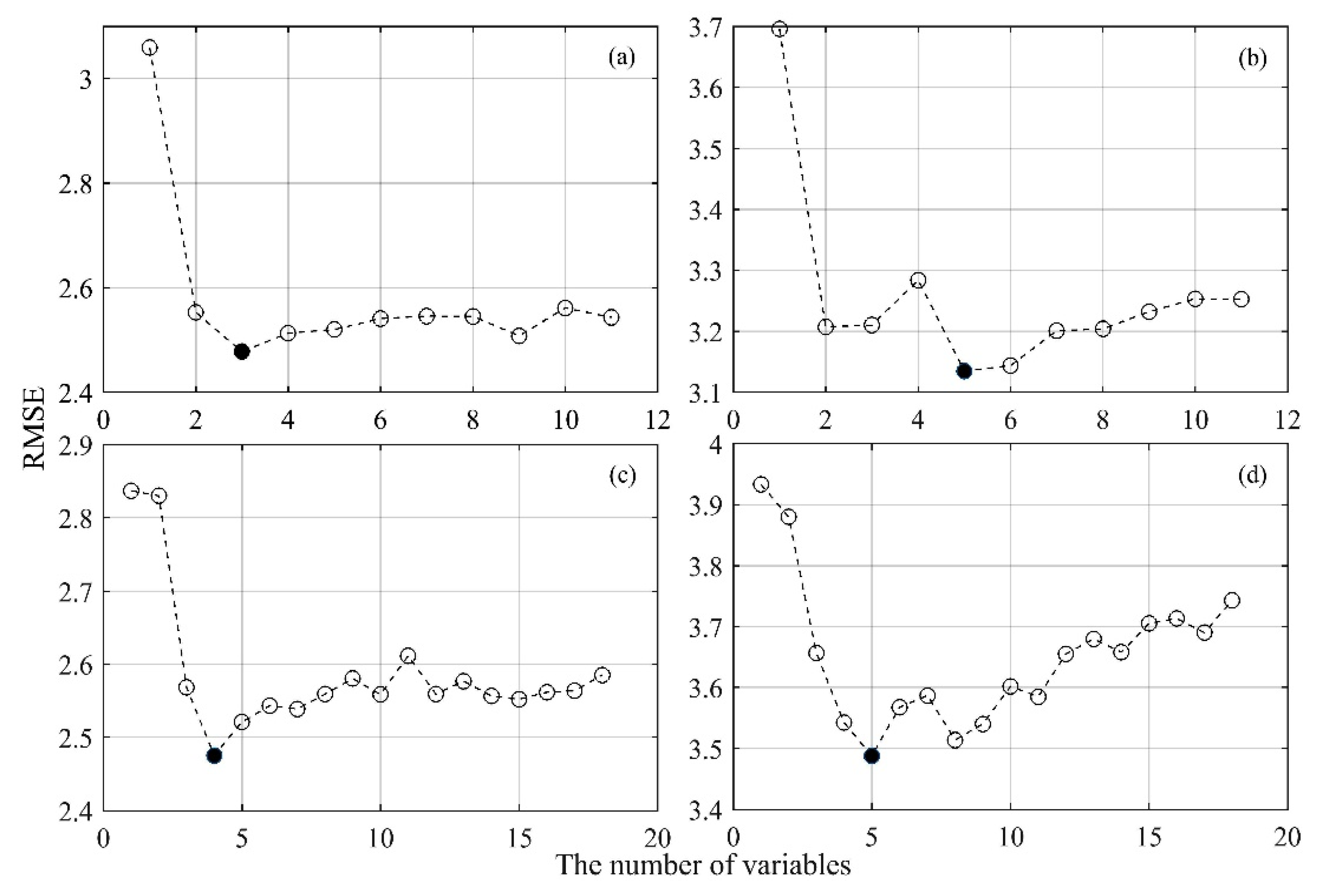
2.7. Variable Selection and Cross-Validation

A feature selection method (RFFS) based on the increase in node purity (IncNodePurity) of the RF model is applied to optimize spectral bands and VIs. RFFS ranks the input features based on IncNodePurity, and the sequential backward search method is then used to remove the least important feature with the smallest IncNodePurity value from the feature set every time. The root mean squared error (RMSE) of the validation set of each iteration is calculated to evaluate model prediction accuracy. After many iterations, the feature set with the minimum RMSE and the fewest variables is ultimately selected. To guarantee the stability of the experimental results, 10-fold cross-validation is used [54]. In the validation process, the order of importance of variables generated by each iteration is selected as the basis for eliminating features, and the average RMSE is calculated to evaluate the generalization and prediction ability of the model.

2.8. Accuracy Assessment

The mean absolute error (MAE, Equation (1)), R2, RMSE, Akaike information criterion (AIC, Equations (2) and (3)), and Bayesian information criterion (BIC, Equations (2) and (4)) are used to comprehensively evaluate the performance of candidate forage N:P ratio models from multiple perspectives. The R2 and RMSE are used to evaluate the accuracy and goodness of fit, respectively, of the simulated and measured forage N:P ratios. MAE is used to assess the modeling errors in estimating the forage N:P ratio [34]. In addition, the AIC and BIC are used to balance the complexity and precision of the estimation model [55,56].
MAE = 1 n | y i y ^ i |
RSS = i = 1 n ( y i y ^ i ) 2
AIC = 2 k + n ln ( R S S / n )
BIC = n ln ( R S S / n ) + k ln ( n )
where RSS represents the residual sum of squares between measured and simulated N:P ratios; y ^ i and y i are the N:P ratios of the validation set for the simulated and measured values, respectively; and n and k are the numbers of observations and variables in the model, respectively.

3. Results

3.1. Variation in the Forage N:P Ratio

The results indicate that the average forage N and P contents in the vigorous growth period (July) are significantly higher than those in the senescing period (November), which indicates that forage N and P gradually decrease in the late growing season, while the average forage N:P ratio shows a pattern contrary to the variation in N and P contents (Table 3). On the whole, the coefficients of variation in forage N, P and N:P ratio in the senescing period are greater than those in the vigorous growth period, which also means that the grassland vegetation has greater spatial heterogeneity in the senescing period.
The forage N:P ratio is significantly correlated with the N and P contents at different growth stages (Table 4), which further supports using the VIs related to N, P and chlorophyll to estimate the forage N:P ratio. The correlation between the forage N:P ratio and P is strong (r = −0.74 in July 2017 and r = −0.59 in November 2017), indicating that the forage N:P ratio mainly depends upon the forage P content. The correlation between forage N and P is not significant (r = 0.17, p = 0.1647) in the vigorous growth period, but there is a weak correlation between them (r = 0.32) in the senescing period, showing that the correlation between forage N and P changes with the growth stage. Compared with the senescing period, the vigorous growth period appears to be a more suitable period for retrieving the forage N:P ratio.

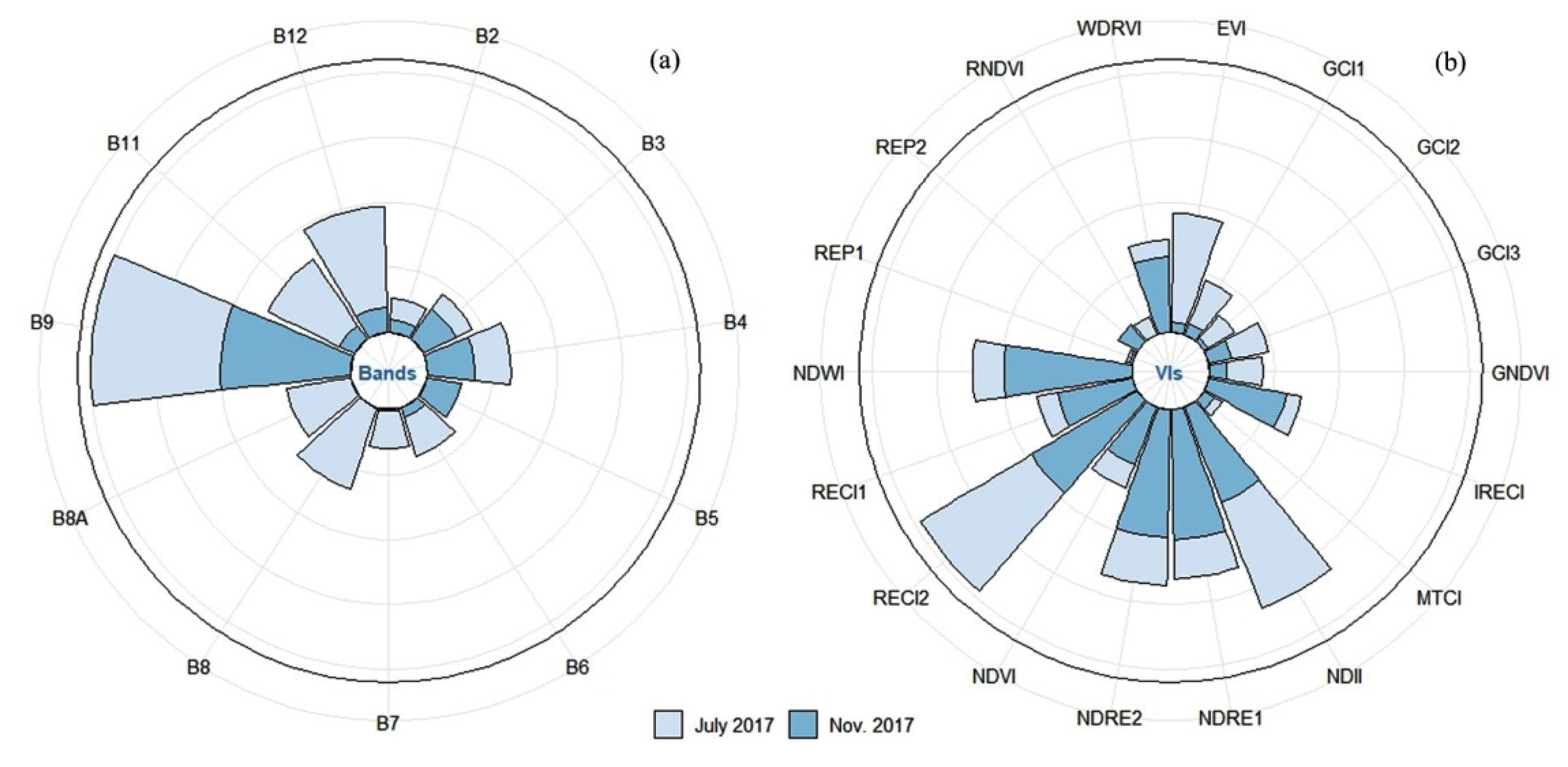
3.2. Predicting the Forage N:P Ratio with Spectral Bands

The results of the forage N:P ratio estimation based on 11 spectral bands at different growth stages are shown in Table 5. Using the RFFS algorithm to optimize the spectral bands slightly increases the performance of modeling the forage N:P ratio and reduces the complexity of the model (i.e., the model has a lower AIC and BIC) compared with those observed for the forage N:P ratio model established with entire bands. As shown in Figure 2 and Figure 3, three bands (B8-NIR, B9-NIR and B12-SWIR) and five bands (B3-Green, B4-Red, B5-Red edge, B9-NIR, and B12-SWIR) are selected as important bands for estimating the forage N:P ratio in the vigorous growth period (July) and the senescing period (November), with R2 values of 0.43 and 0.55, respectively.
Figure 3a shows the analysis results for the relative importance of different bands in the estimation of the forage N:P ratio. Overall, B9 and B12 play an important part in the estimation of the forage N:P ratio during the vigorous growth period and the senescing period, especially B9, which greatly contributes to forage N:P ratio estimation. B11 and B12 are more important for estimating the forage N:P ratio in the vigorous growth period, but they are less sensitive to the forage N:P ratio detection in the senescing period. In addition, B3 and B5 have a good potential in retrieving the forage N:P ratio in the vigorous growth period, but they have no significant effect on the estimation of the N:P ratio in the senescing period. It can be concluded that the bands sensitive to the estimation of the forage N:P ratio in the vigorous growth period are mainly distributed in the NIR and SWIR regions. Moreover, some bands located in the red (B4) and red-edge (B5) regions also significantly influence the estimation of the forage N:P ratio in the senescing period, in addition to the NIR and SWIR regions.

3.3. Predicting the Forage N:P Ratio with Sentinel-2 Vegetation Indices

The results of the forage N:P ratio estimation based on 18 VIs at different growth stages are shown in Table 6. Using the RFFS algorithm to optimize the VIs slightly increases the performance of modeling the forage N:P ratio and reduces the complexity of the model (i.e., the model has a lower AIC and BIC) compared with those observed for the forage N:P ratio model established with entire VIs. As shown in Figure 2 and Figure 3, four VIs (enhanced vegetation index (EVI), green chlorophyll index (GCI1), normalized difference infrared index (NDII) and red-edge chlorophyll index (RECI2)) and five VIs (normalized difference red edge 1 (NDRE1), NDRE2, RECI2, normalized difference water index (NDWI) and wide dynamic range vegetation index (WDRVI)) are selected as important VIs for estimating the forage N:P ratio in the vigorous growth period (July) and the senescing period (November), with R2 values of 0.43 and 0.42, respectively.
Figure 3b shows the analysis results for the relative importance of different VIs for estimating forage N:P ratio. Overall, RECI2 is important for the forage N:P ratio estimation in both the vigorous growth period and the senescing period. NDII and RECI2 significantly contribute to the forage N:P ratio estimation during the vigorous growth period, and NDWI, RECI2, NDRE1 and NDRE2 are the four most important VIs for the forage N:P ratio estimation in the senescing period. In addition, the seven VIs sensitive to the forage N:P ratio in the vigorous growth period all include the NIR band (B8 or B8A). Among the 5 VIs sensitive to the forage N:P ratio in the senescing period, B5 and B8A in the red-edge and NIR regions are the most frequent bands, respectively. These results indicate that the NIR band has a good potential in estimating the forage N:P ratio as a whole.

3.4. Predicting the Forage N:P Ratio with a Combination of Spectral Bands and Vegetation Indices

The optimized spectral bands and VIs are integrated to establish an RF model for the forage N:P ratio estimation at different growth stages (Table 7). Compared with the forage N:P ratio model established by using the optimized spectral bands (n = 3) or VIs (n = 4) alone, the prediction accuracy of the integrated model (R2 = 0.49) is improved by 0.06 in the vigorous growth period (July). The accuracy of the integrated N:P ratio model (R2 = 0.59) is improved by 0.04 in the senescing period (November) compared with the model that used the optimized spectral bands (n = 5) or VIs (n = 5) alone. This indicates that the integration of optimized spectral bands and VIs increases the estimation accuracy of the forage N:P ratio.

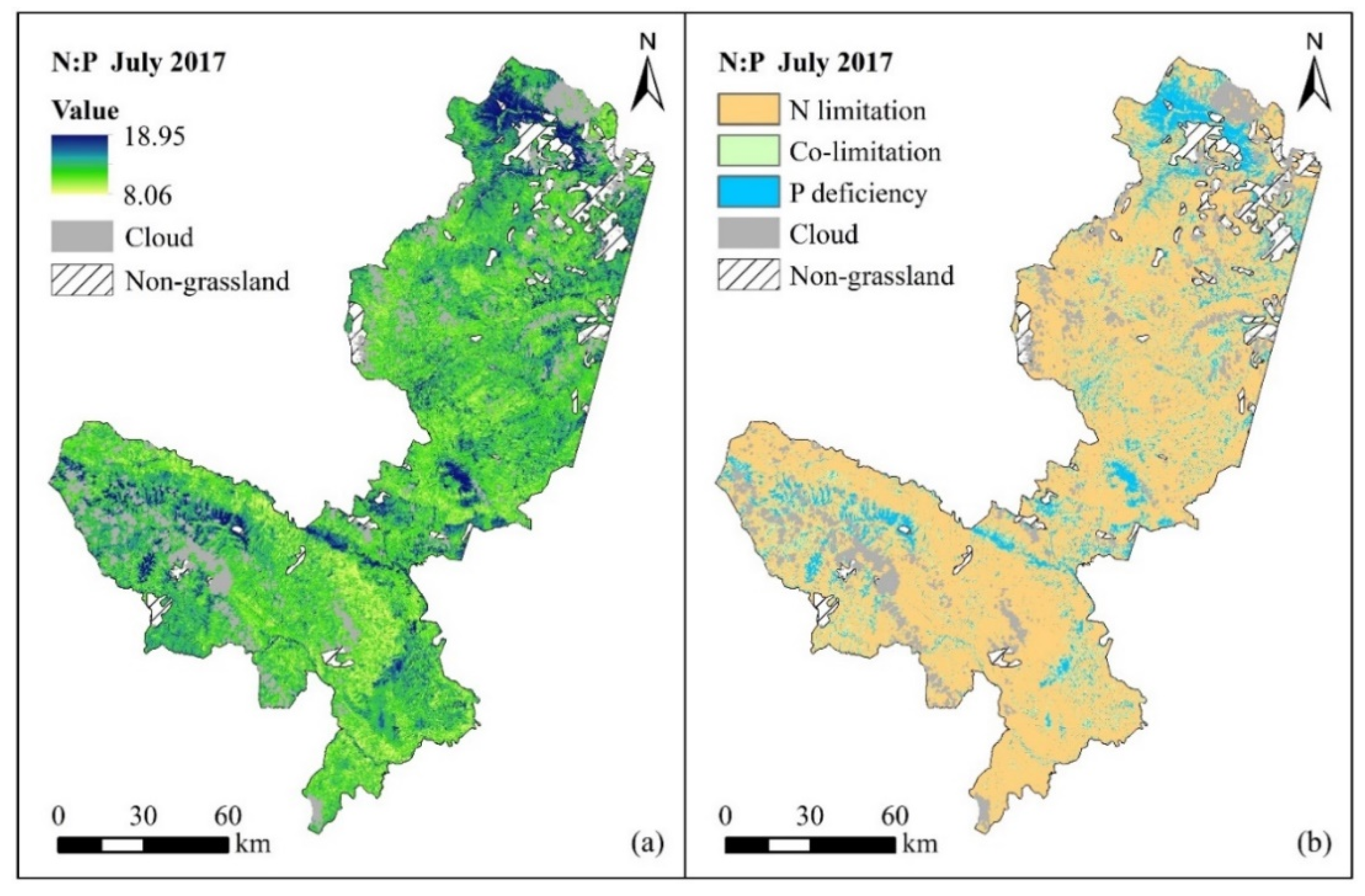
3.5. Mapping of Potential Forage N and P Limitation

According to the integrated model of the forage N:P ratio in the two periods mentioned above, the spatial distribution of the forage N:P ratio is mapped based on Sentinel-2 MSI images. The spatial distribution and nutrient limitation of the forage N:P ratio at different growth stages are shown in Figure 4 (the vigorous growth period) and Figure 5 (the senescing period). The results indicate that the forage N:P ratio ranges from 8.06 to 18.95 in the vigorous growth period. Overall, the growth of forage in most of the study area is limited by N (N:P < 14), the nutrient condition of forage in the local area (i.e., northern Xiahe County, southern Luqu County and northwestern Maqu County) is affected by P deficiency (N:P > 16), and the forage growth in very few areas is restricted by both N and P (14 < N:P < 16) (Figure 4). Moreover, the forage N:P ratio is between 7.75 and 22 in the senescing period (Figure 5). Comparative analysis of the spatial distribution of the forage N:P ratio in the above two periods shows that the forage N:P ratio increases in most areas and decreases slightly in local areas, which suggests that the P content in forage is more deficient than the N content when grassland vegetation stops growing.

4. Discussion

4.1. Potential of Sentinel-2 Spectral Bands and Vegetation Indices in Estimating the Forage N:P Ratio

This study shows that the Sentinel-2 spectral bands are mainly distributed in the NIR and SWIR regions have an important contribution to the forage N:P estimation of alpine grassland, and some spectral bands located in the red and red-edge regions have a great influence on estimating the forage N:P ratio in the senescing period. In addition, some VIs (such as RECI2) constructed by the Sentinel-2 spectral bands in the red and NIR regions have a good potential in the inversion of the forage N:P ratio. Previous studies have shown that there is a significant correlation between the spectral reflectance of the red-edge and NIR regions and the N content in plant leaves [57,58]. The bands that are sensitive to the P content in vegetation are mainly distributed in the NIR and SWIR regions [59], and VIs based on the red-edge are important variables for predicting the N content in leaves [4]. At different growth stages, the N:P ratio is significantly correlated with the forage N and P contents (Table 4). Therefore, the bands sensitive to N and P may also be applicable to the estimation of N:P ratio in forage. Romoelo et al. [11] estimated the N:P of savanna forages based on hyperspectral data and found that the wavebands were distributed in the SWIR region had a higher sensitivity to N:P in leaves, which is similar to our finding. In different growth stages of grassland, the optimization results of spectral bands based on the RF algorithm show that both B9 and B12 are important bands for estimating the forage N:P ratio. The potential of B12 in estimating the forage N:P ratio can be understood by the absorption feature of N near 2180 nm.
The detection of the forage N using remote sensing technology is generally associated with the absorption of chlorophyll, and usually includes the spectral regions related to chlorophyll detection (i.e., the red-edge and NIR regions) [33]. Previous studies have shown that some known specific absorption bands for chlorophyll, N, and proteins (i.e., 640 nm, 660 nm, 910 nm, and 1510 nm) can be successfully employed to retrieve the forage N content [11,60,61]. The specific absorption features of P are mainly distributed in the NIR and SWIR regions, having broad application prospect in estimating forage P [6,62]. The detection of forage P applying hyperspectral measurements could be related to the stoichiometry (i.e., indirect estimation according to the relationship between other biochemical parameters and P in forage) [63,64]. Preliminary results show the forage N:P ratio is significant correlated with the N and P contents (Table 4), which further supports the feasibility of using the spectral variables related to N, P and chlorophyll to indirectly estimate the forage N:P ratio.
This study confirms that it is feasible to use Sentinel-2 MSI spectral bands and VIs to estimate the forage N:P ratio, and combining optimized spectral bands and VIs further increases the estimation accuracy of the forage N:P ratio. Previous studies have also shown that combining spectral bands and VIs improves the estimation accuracy of vegetation biochemical parameters [4,34], which benefits from enhancing some of the most important variables and integrating effective information to obtain the best results.

4.2. Effects of Different Seasons on Forage N:P Inversion in Natural Alpine Grasslands

The growth and developmental stages of forage directly affect its nutrient content, thereby affecting the feed intake and production performance of animals. This study shows that the average forage N and P contents in the vigorous growth period (July) are significantly higher than those in the senescing period (November) at different growth stages. Many studies have also found that the contents of N, P and protein in forage gradually decrease as plant grows [65]. For example, the P content of eight forages in the Alxa Desert steppe show regular seasonal dynamics; that is, the P content gradually decreases with the advancement of the growth period [66], and the N content in the aboveground part of plants decreases during the plant growth season (May to September) [67]. The forage N content gradually decreases as the forage grows in alpine grassland, especially the forage N that decreases rapidly during the senescing period [68]. In the late growth season, with the expansion of plants, the forage gradually withers, cell senescence occurs, and fiber material increases, resulting in the dilution effect of elements [69]. In addition, plants gradually stop growing after entering the senescing period, and some of the aboveground nutrients are transferred underground for storage to supply the consumption of plants in non-growing period and nutrients needed for plant germination in the coming year [70]. This study reveals that the growth of forage is mainly limited by N during the vigorous growth period in alpine grasslands. With the gradual senescing of forage, the N:P ratio increases significantly, and the vegetation gradually changes from being N limited to P deficient. Especially at the end of the growing season, the limitation effect of P on vegetation growth is greater than that of N, which is potentially related to P being fixed in plant roots during the senescence of forage.
This study shows that the integrated forage N:P ratio model achieves ideal estimation accuracy in both the vigorous growth period (R2 = 0.49) and the senescing period (R2 = 0.59) (Table 7). This finding indicates that some spectral bands and VIs from Sentinel-2 can capture nutrient limitation information for forage growth to a certain extent. Using multispectral data to estimate the forage canopy N:P ratio provides an indirect measurement of the deficiency status of N and P in grassland vegetation, and some spectral bands and VIs that are sensitive to forage N, P and chlorophyll play an important role in N:P ratio estimation [11,26]. The biomass of alpine grasslands reaches its maximum and grazing intensity is relatively high during the vigorous growth period. In terms of practical applications, it is of more practical significance to use remote sensing data to monitor forage growth in this stage than in other stages at a regional scale. In general, the nutrient content of forage decreases and the quality deteriorates during the senescing period, and the canopy spectrum is easily affected by soil and other background factors, which will reduce the sensitivity of the spectral bands and VIs to forage N and P [68,71]. According to our research results, the integrated forage N:P ratio model performs better in the senescing period than in the vigorous growth period, which is potentially attributable to the limited number of sample sites, the optimization of model parameters, and large spatial heterogeneity of grassland. Subsequent research will also explore this problem more deeply based on multisource satellite data and multiple machine learning algorithms.

4.3. Future Perspectives

Although this study maps the spatial distribution of the forage N:P ratio in the vigorous growth period and the senescing period on a regional scale, it is also necessary to understand the potential limitations of this method. The empirical estimation model of vegetation biochemical parameters is susceptible to the spatial heterogeneity of the study area, which reduces the generalization performance of the model in other regions, and therefore still faces many challenges in practical application [19,72]. Due to the cloudy and rainy weather in summer, the grass canopy spectrum and the cloud cover of the optical satellite images are seriously limited by the weather conditions, which confines the remote sensing monitoring of vegetation growth in the study area to a certain extent.
For vegetation applications, hyperspectral sensors (i.e., HYMAP, Hyperion, AISA Eagle and Gaofen-5) can provide abundant spectral information and detect minute spectral features that are masked by the broad bands of satellites [73]. In addition, spectral bands are favorable to the calculation of the red-edge position and narrow band indices, important for vegetation biochemical parameters assessments [74]. Moreover, hyperspectral data have received extensive attention for species discrimination and mapping subtle variations in vegetation biochemical information. However, the high cost and the small swath width involved limits its usage to small spatial extents [14,27]. The recent trend is that hyperspectral data is gradually shifting towards to affordable multispectral sensors with strategic bands (i.e., RapidEye, WorldView-2, Sentinel-2A/B and Gaofen-6), which capable of retrieving plant macronutrients [75,76,77]. Near-surface unmanned aerial vehicle (UAV) remote sensing systems have the advantages of a small size, wide applications and high flexibility, which can overcome the limitations of conventional ground observation-based methods [78,79]. Therefore, exploring integrated monitoring technology for grass biochemical parameters based on near-surface UAV images and multisource, multitemporal and high-resolution satellite data will be the focus of future research.
As RTMs are capable of explaining the interaction and transfer of radiation inside the canopy according to the laws of physics, they offer a specific connection between the canopy reflectance and the vegetation biochemical parameters [80]. A physically based models (i.e., PROSPECT and LIBERTY) have the advantages that a large simulated spectra database can be generated by changing the input parameters [81], which may be applied to other areas. Many studies show that the model inversion has certain potential for estimating vegetation biophysical parameters in heterogeneous grasslands applying hyperspectral data [17,82]. The combination of empirical and physically based models is a reliable approach for estimating forage N and P, although its generalization performance needs to be verified by other data sets.

5. Conclusions

Based on high-resolution multispectral satellite data and an RF machine learning algorithm, this study evaluates the feasibility of using Sentinel-2 MSI spectral bands and VIs to retrieve the forage N:P ratio of alpine grassland on a regional scale. The results indicate that combining optimized spectral bands and VIs increases the accuracy of the forage N:P ratio estimation in comparison with that of models using spectral bands or VIs alone. In addition, the Sentinel-2 spectral bands are mainly distributed in the NIR and SWIR regions have a valuable contribution toward estimating the forage N:P ratio, and some spectral bands located in the red and red-edge regions greatly influence the forage N:P ratio in the senescing period. This study demonstrates the practicality and feasibility of using Sentinel-2 spectral bands and VIs to directly estimate the forage N:P ratio at regional scales. Moreover, airborne and satellite data can be integrated to diagnose the seasonal variations of nutrition limitation at a landscape level in the alpine grassland ecosystem of the Tibetan Plateau and thus represents a promising future development trend.

Author Contributions

All authors contributed significantly to this manuscript. J.G. (Jinlong Gao) and T.L. designed this study. J.G. (Jinlong Gao), J.L., M.H., J.G. (Jing Ge), Q.F. and C.W. were responsible for the paper writing, data analysis, and processing. W.L. made valuable editing and revisions of the paper. All authors have read and agreed to the published version of the manuscript.

Funding

This research was funded by the National Natural Science Foundation of China (31672484 and 31702175), the Program for Changjiang Scholars and Innovative Research Team in University (IRT_17R50), and the 111 Project (B12002).

Conflicts of Interest

All coauthors declare that there are no conflicts of interests.

References

  1. Blackburn, G.A. Spectral indices for estimating photosynthetic pigment concentrations: A test using senescent tree leaves. Int. J. Remote Sens. 1998, 19, 657–675. [Google Scholar] [CrossRef]
  2. Ullah, S.; Si, Y.L.; Schlerf, M.; Skidmore, A.K.; Shafique, M.; Iqbal, I.K. Estimation of grassland biomass and nitrogen using MERIS data. Int. J. Appl. Earth Obs. Geoinf. 2012, 19, 196–204. [Google Scholar] [CrossRef]
  3. Richardson, A.J.; Everitt, J.H.; Gausman, H.W. Radiometric estimation of biomass and nitrogen content of alicia grass. Remote Sens. Environ. 1983, 13, 179–184. [Google Scholar] [CrossRef]
  4. Ramoelo, A.; Cho, M.A.; Mathieu, R.; Madonsela, S.; Van De Kerchove, R.; Kaszta, Z.; Wolff, E. Monitoring grass nutrients and biomass as indicators of rangeland quality and quantity using random forest modelling and WorldView-2 data. Int. J. Appl. Earth Obs. Geoinf. 2015, 43, 43–54. [Google Scholar] [CrossRef]
  5. Walker, A.P.; Beckerman, A.P.; Gu, L.; Kattge, J.; Cernusak, L.A.; Domingues, T.F.; Scales, J.C.; Wohlfahrt, G.; Wullschleger, S.D.; Woodward, F.I. The relationship of leaf photosynthetic traits–vcmax and Jmax–to leaf nitrogen, leaf phosphorus, and specific leaf area: A meta-analysis and modeling study. Ecol. Evol. 2014, 4, 3218–3235. [Google Scholar] [CrossRef] [Green Version]
  6. Gao, J.L.; Meng, B.P.; Liang, T.G.; Feng, Q.S.; Ge, J.; Yin, J.P.; Wu, C.X.; Cui, X.; Hou, M.J.; Liu, J.; et al. Modeling alpine grassland forage phosphorus based on hyperspectral remote sensing and a multi-factor machine learning algorithm in the east of Tibetan Plateau. China. ISPRS J. Photogramm. Remote Sens. 2019, 147, 104–117. [Google Scholar] [CrossRef]
  7. Koerselman, W.; Meuleman, A.F.M. The vegetation N:P ratio: A new tool to detect the nature of nutrient limitation. J. Appl. Ecol. 1996, 33, 1441–1450. [Google Scholar] [CrossRef]
  8. Olde Venterink, H.; Wassen, M.J.; Verkroost, A.W.M.; De Ruiter, P.C. Species richness-productivity patterns differ between N-, P-, and K-limited wetlands. Ecology 2003, 84, 2191–2199. [Google Scholar] [CrossRef]
  9. He, J.S.; Wang, L.; Flynn, D.F.B.; Wang, X.P.; Ma, W.H.; Fang, J.Y. Leaf nitrogen:phosphorus stoichiometry across Chinese grassland biomes. Oecologia 2008, 155, 301–310. [Google Scholar] [CrossRef]
  10. Tessier, J.T.; Raynal, D.J. Use of nitrogen to phosphorus ratios in plant tissue as an indicator of nutrient limitation and nitrogen saturation. J. Appl. Ecol. 2003, 40, 523–534. [Google Scholar] [CrossRef]
  11. Ramoelo, A.; Skidmore, A.K.; Schlerf, M.; Heitkonig, I.M.; Mathieu, R.; Cho, M.A. Savanna grass nitrogen to phosphorous ratio estimation using field spectroscopy and the potential for estimation with imaging spectroscopy. Int. J. Appl. Earth Obs. Geoinf. 2013, 23, 334–343. [Google Scholar] [CrossRef]
  12. Wassen, M.J.; Venterink, H.O.; Lapshina, E.D.; Tanneberger, F. Endangered plants persist under phosphorus limitation. Nature 2005, 437, 547–550. [Google Scholar] [CrossRef] [PubMed]
  13. Fujita, Y.; Venterink, H.O.; van Bodegom, P.M.; Douma, J.C.; Heil, G.W.; Holzel, N.; Jablonska, E.; Kotowski, W.; Okruszko, T.; Pawlikowski, P.; et al. Low investment in sexual reproduction threatens plants adapted to phosphorus limitation. Nature 2014, 505, 82–86. [Google Scholar] [CrossRef] [PubMed]
  14. Mutanga, O.; Dube, T.; Ahmed, F. Progress in remote sensing: Vegetation monitoring in South Africa. S. Afr. Geogr. J. 2016, 98, 461–471. [Google Scholar] [CrossRef]
  15. Ma, W.Y.; Wang, X.M. Progress on grassland chlorophyll content estimation by hyperspectral analysis. Prog. Geogr. 2016, 35, 25–34. [Google Scholar]
  16. Skidmore, A.K. Taxonomy of environmental models in the spatial sciences. In Environmental Modelling with GIS and Remote Sensing; Skidmore, A.K., Ed.; Taylor and Francis: London, UK, 2002; pp. 2–7. [Google Scholar]
  17. Wang, Z.H.; Skidmore, A.K.; Wang, T.J.; Darvishzadeh, R.; Hearne, J. Applicability of the PROSPECT model for estimating protein and cellulose + lignin in fresh leaves. Remote Sens. Environ. 2015, 168, 205–218. [Google Scholar] [CrossRef]
  18. Penuelas, J.; Gamon, J.A.; Freeden, A.L.; Merino, J.; Field, C. Reflectance indices associated with physiological changes in nitrogen and water-limited sunflower leaves. Remote Sens. Environ. 1994, 48, 135–146. [Google Scholar] [CrossRef]
  19. Mutanga, O. Hyperspectral Remote Sensing of Tropical Grass Quality and Quantity. Ph.D. Thesis, International Institute for Geoinformation Science and Earth Observation and Wageningen University, Wageningen, The Netherlands, 7 April 2004. [Google Scholar]
  20. Filella, I.; Penuelas, J. The red edge position and shape as indicators of plant chlorophyll content, biomass and hydric status. Int. J. Remote Sens. 1994, 15, 1459–1470. [Google Scholar] [CrossRef]
  21. Danson, F.M.; Plummer, S.E. Red edge response to forest leaf area index. Int. J. Remote Sens. 1995, 16, 183–188. [Google Scholar] [CrossRef]
  22. Curran, P.J.; Dungan, J.L.; Macler, B.A.; Plummer, S.E. The effect of a Red leaf pigment on the relationship between red edge and chlorophyll concentration. Remote Sens. Environ. 1991, 35, 69–76. [Google Scholar] [CrossRef]
  23. Ramoelo, A. Savanna Grass Quality-Remote Sensing Estimation from Local to Regional Scale. Ph.D. Thesis, University of Twente, Enschede, The Netherlands, 2012. [Google Scholar]
  24. Gao, J.L.; Liang, T.G.; Liu, J.; Yin, J.P.; Ge, J.; Hou, M.J.; Feng, Q.S.; Wu, C.X.; Xie, H.J. Potential of hyperspectral data and machine learning algorithms to estimate the forage carbon-nitrogen ratio in an alpine grassland ecosystem of the Tibetan Plateau. ISPRS J. Photogramm. Remote Sens. 2020, 163, 362–374. [Google Scholar] [CrossRef]
  25. Gökkaya, K.; Thomas, V.; Noland, T.; McCaughey, H.; Morrison, I.; Treitz, P. Mapping continuous forest type variation by means of correlating remotely sensed metrics to canopy N:P ratio in a boreal mixed wood forest. Appl. Veg. Sci. 2015, 18, 143–157. [Google Scholar] [CrossRef]
  26. Loozen, Y.; Karssenberg, D.; de Jong, S.M.; Wang, S.Q.; van Dijk, J.; Wassen, M.J.; Rebel, K.T. Exploring the use of vegetation indices to sense canopy nitrogen to phosphorous ratio in grasses. Int. J. Appl. Earth Obs. Geoinf. 2019, 75, 1–14. [Google Scholar] [CrossRef]
  27. Tong, Q.X.; Xue, Y.Q.; Zhang, L.F. Progress in hyperspectral remote sensing science and technology in China over the past three decades. IEEE J. Sel. Top. Appl. Earth Obs. Remote Sens. 2013, 7, 70–91. [Google Scholar] [CrossRef]
  28. Lehnert, L.W.; Meyer, H.; Wang, Y.; Miehe, G.; Thies, B.; Reudenbach, C.; Bendic, J. Retrieval of grassland plant coverage on the Tibetan Plateau based on a multiscale, multi-sensor and multi-method approach. Remote Sens. Environ. 2015, 164, 197–207. [Google Scholar] [CrossRef]
  29. Yang, S.X.; Feng, Q.S.; Liang, T.G.; Liu, B.K.; Zhang, W.J.; Xie, H.J. Modeling grassland above-ground biomass based on artificial neural network and remote sensing in the Three-River Headwaters Region. Remote Sens. Environ. 2017, 204, 448–455. [Google Scholar] [CrossRef]
  30. Meng, B.P.; Gao, J.L.; Liang, T.G.; Cui, X.; Ge, J.; Yin, J.P.; Feng, Q.S.; Xie, H.J. Modeling of alpine grassland cover based on unmanned aerial vehicle technology and multi-factor methods: A case study in the east of Tibetan Plateau, China. Remote Sens. 2018, 10, 320. [Google Scholar] [CrossRef] [Green Version]
  31. Ramoelo, A.; Skidmore, A.K.; Cho, M.A.; Schlerf, M.; Mathieu, R.; Heitkonig, I.M. Regional estimation of savanna grass nitrogen using the red-edge band of the spaceborne RapidEye sensor. Int. J. Appl. Earth Obs. Geoinf. 2012, 19, 151–162. [Google Scholar] [CrossRef]
  32. Shoko, C.; Mutanga, O. Examining the strength of the newly-launched Sentinel 2 MSI sensor in detecting and discriminating subtle differences between C3 and C4 grass species. ISPRS J. Photogramm. Remote Sens. 2017, 129, 32–40. [Google Scholar] [CrossRef]
  33. Schlemmer, M.; Gitelson, A.; Schepers, J.; Ferguson, R.; Peng, Y.; Shanahan, J.; Rundquist, D. Remote estimation of nitrogen and chlorophyll contents in maize at leaf and canopy levels. Int. J. Appl. Earth Obs. Geoinf. 2013, 25, 47–54. [Google Scholar] [CrossRef] [Green Version]
  34. Chemura, A.; Mutanga, O.; Odindi, J.; Kutywayo, D. Mapping spatial variability of foliar nitrogen in coffee (Coffea arabica L.) plantations with multispectral Sentinel-2 MSI data. ISPRS J. Photogramm. Remote Sens. 2018, 138, 1–11. [Google Scholar] [CrossRef]
  35. Singh, L.; Mutanga, O.; Mafongoya, P.; Peerbhay, K.Y. Multispectral mapping of key grassland nutrients in KwaZulu-Natal. S. Afr. J. Spat. Sci. 2018, 63, 155–172. [Google Scholar] [CrossRef]
  36. Clevers, J.G.P.W.; Gitelson, A.A. Remote estimation of crop and grass chlorophyll and nitrogen content using red-edge bands on sentinel-2 and-3. Int. J. Appl. Earth Obs. Geoinf. 2013, 23, 344–351. [Google Scholar] [CrossRef]
  37. Sakowska, K.; Juszczak, R.; Gianelle, D. Remote sensing of grassland biophysical parameters in the context of the Sentinel-2 satellite mission. J. Sens. 2016, 2016, 4612809. [Google Scholar] [CrossRef] [Green Version]
  38. Rouse, J.; Haas, R.H.; Schell, J.A.; Deering, D.W. Monitoring vegetation systems in the Great Plains with ERTS. In Proceedings of the Third Earth Resources Technology Satellite-1 Symposium, Greenbelt, MD, USA, 10–14 December 1973. [Google Scholar]
  39. Hardisky, M.A.; Klemas, V.; Smart, R.M. The influences of soil salinity, growth form, and leaf moisture on the spectral reflectance of spartina alterniflora canopies. Photogramm. Eng. Remote Sens. 1983, 49, 77–83. [Google Scholar]
  40. Gao, B.C. NDWI—A normalized difference water index for remote sensing of vegetation liquid water from space. Remote Sens. Environ. 1996, 58, 257–266. [Google Scholar] [CrossRef]
  41. Sims, D.A.; Gamon, J.A. Relationships between leaf pigment content and spectral reflectance across a wide range of species, leaf structures and developmental stages. Remote Sens. Environ. 2002, 81, 337–354. [Google Scholar] [CrossRef]
  42. Barnes, E.M.; Clarke, T.R.; Richards, S.E.; Colaizzi, P.D.; Haberland, J.; Kostrzewski, M.; Waller, P.; Choi, C.; Riley, E.; Thompson, T.; et al. Coincident detection of crop water stress, nitrogen status and canopy density using ground-based multispectral data. In Proceedings of the Fifth International Conference on Precision Agriculture, Bloomington, MN, USA, 16–19 July 2000. [Google Scholar]
  43. Gitelson, A.A.; Merzlyak, M.N. Quantitative estimation of chlorophyll using reflectance spectra. J. Photochem. Photobiol. 1994, 22, 247–252. [Google Scholar] [CrossRef]
  44. Gitelson, A.A.; Kaufman, Y.J.; Merzlyak, M.N. Use of a green channel in remote sensing of global vegetation from EOSMODIS. Remote Sens. Environ. 1996, 58, 289–298. [Google Scholar] [CrossRef]
  45. Huete, A.; Didan, K.; Miura, T.; Rodriguez, E.P.; Gao, X.; Ferreira, L.G. Overview of the radiometric and biophysical performance of the MODIS vegetation indices. Remote Sens. Environ. 2002, 83, 195–213. [Google Scholar] [CrossRef]
  46. Frampton, W.J.; Dash, J.; Watmough, G.; Milton, E.J. Evaluating the capabilities of Sentinel-2 for quantitative estimation of biophysical variables in vegetation. ISPRS J. Photogramm. Remote Sens. 2013, 82, 83–92. [Google Scholar] [CrossRef] [Green Version]
  47. Guyot, G.; Baret, F. Utilisation de la haute resolution spectrale pour suivre l’etat des couverts vegetaux. In Proceedings of the 4th International Colloquium Spectral Signatures of Objects in Remote Sensing, Aussois, France, 18–22 January 1988. [Google Scholar]
  48. Dash, J.; Curran, P.J. The MERIS terrestrial chlorophyll index. Int. J. Remote Sens. 2004, 25, 5403–5413. [Google Scholar] [CrossRef]
  49. Gitelson, A.A.; Viña, A.; Ciganda, V.; Rundquist, D.C.; Arkebauer, T.J. Remote estimation of canopy chlorophyll content in crops. Geophys. Res. Lett. 2005, 32, L08403. [Google Scholar] [CrossRef] [Green Version]
  50. Gitelson, A.A.; Gritz, Y.; Merzlyak, M.N. Relationships between leaf chlorophyll content and spectral reflectance and algorithms for nondestructive chlorophyll assessment in higher plant leaves. J. Plant Physiol. 2003, 160, 271–282. [Google Scholar] [CrossRef]
  51. Gitelson, A.A. Wide dynamic range vegetation index for remote quantification of biophysical characteristics of vegetation. J. Plant Physiol. 2004, 161, 165–173. [Google Scholar] [CrossRef] [Green Version]
  52. Breiman, L. Random forests. Mach. Learn. 2001, 45, 5–32. [Google Scholar] [CrossRef] [Green Version]
  53. Lebedev, A.; Westman, E.; Van Westen, G.; Kramberger, M.; Lundervold, A.; Aarsland, D.; Soininen, H.; Kłoszewska, I.; Mecocci, P.; Tsolaki, M. Random Forest ensembles for detection and prediction of Alzheimer’s disease with a good between-cohort robustness. NeuroImage Clin. 2014, 6, 115–125. [Google Scholar] [CrossRef] [Green Version]
  54. Kohavi, R. A study of cross-validation and bootstrap for accuracy estimation and model selection. In Proceedings of the 14th International Joint Conference on Artificial Intelligence, Montreal, QC, Canada, 20–25 August 1995; Volume 2, pp. 1137–1143. [Google Scholar]
  55. Akaike, H. Information theory and an extension of the maximum likelihood principle. In International Symposium on Information Theory; Akademiai, K., Ed.; Springer: New York, NY, USA, 1973; pp. 610–624. [Google Scholar]
  56. Schwarz, G. Estimating the dimension of a model. Ann. Statist. 1978, 6, 461–464. [Google Scholar] [CrossRef]
  57. Ollinger, S.V.; Richardson, A.D.; Martin, M.E.; Hollinger, D.Y.; Frolking, S.E.; Reich, P.B.; Plourde, L.C.; Katul, G.G.; Munger, J.W.; Oren, R. Canopy nitrogen, carbon assimilation, and albedo in temperate and boreal forests: Functional relations and potential climate feedbacks. Proc. Natl. Acad. Sci. USA 2008, 105, 19336–19341. [Google Scholar] [CrossRef] [Green Version]
  58. Lepine, L.C.; Ollinger, S.V.; Ouimette, A.P.; Martin, M.E. Examining spectral reflectance features related to foliar nitrogen in forests: Implications for broadscale nitrogen mapping. Remote Sens. Environ. 2016, 173, 174–176. [Google Scholar] [CrossRef]
  59. Mutanga, O.; Kumar, L. Estimating and mapping grass phosphorus concentration in an African savanna using hyperspectral image data. Int. J. Remote Sens. 2007, 28, 4897–4911. [Google Scholar] [CrossRef]
  60. Curran, P.J. Remote sensing of foliar chemistry. Remote Sens. Environ. 1989, 30, 271–278. [Google Scholar] [CrossRef]
  61. Knox, N. Observing Temporal and Spatial Variability of Forage Quality. Ph.D. Thesis, Faculty Geo-Information Science and Earth Observation and Twente University, Enschede, The Netherlands, 28 October 2010. [Google Scholar]
  62. Ramoelo, A.; Skidmore, A.K.; Schlerf, M.; Mathieu, R.; Heitkönig, I.M.A. Water removed spectra increase the retrieval accuracy when estimating savanna grass nitrogen and phosphorus concentrations. ISPRS J. Photogramm. Remote Sens. 2011, 66, 408–417. [Google Scholar] [CrossRef]
  63. Daufresne, T.; Loreau, M. Plant–herbivore interactions and ecological stoichiometry: When do herbivores determine plant nutrient limitation. Ecol. Lett. 2001, 4, 196–206. [Google Scholar] [CrossRef]
  64. Elser, J.J.; Dobberfuhl, D.R.; MacKay, N.A.; Schampel, J.H. Organism size, life history, and N:P stoichiometry. BioScience 1996, 46, 674–684. [Google Scholar] [CrossRef] [Green Version]
  65. Aerts, R. Nutrients resorption from senescing leaves of perennials: Are these general patterns? J. Ecol. 1996, 84, 597–608. [Google Scholar] [CrossRef]
  66. Wu, K.S.; Fu, H.; Zhang, X.Y.; Niu, D.C.; Ta, L.T. The seasonal dynamics of nutrient contents and the nutrition balanced values in the eight forage species in the Alxa desert grassland. Arid Zone Res. 2010, 2, 257–262. [Google Scholar] [CrossRef]
  67. Chen, J.X. Alpine Meadow Soil Nitrogen Seasonal Dynamics in Eastern Qinghai-Tibetan Plateau. Ph.D. Thesis, Sichuan Normal University, Sichuan, China, 1 May 2007. [Google Scholar]
  68. Gao, J.L.; Liang, T.G.; Yin, J.P.; Ge, J.; Feng, Q.S.; Wu, C.X.; Hou, M.J.; Liu, J.; Xie, H.J. Estimation of alpine grassland forage nitrogen coupled with hyperspectral characteristics during different growth periods on the Tibetan Plateau. Remote Sens. 2019, 11, 2085. [Google Scholar] [CrossRef] [Green Version]
  69. Shi, Y.; Ma, Y.L.; Ma, W.H.; Liang, C.Z.; Zhao, X.Q.; Fang, J.Y.; He, J.S. Large scale patterns of forage yield and quality across Chinese grasslands. Chin. Sci. Bull. 2013, 58, 1187–1199. [Google Scholar] [CrossRef] [Green Version]
  70. Zhang, J.X.; Cao, G.M. The nitrogen cycle in an alpine meadow ecosystem. Acta Ecol. Sin. 1999, 19, 509–513. [Google Scholar]
  71. Yang, X.H.; Guo, X.L. Quantifying responses of spectral vegetation indices to dead materials in mixed grasslands. Remote Sens. 2014, 6, 4289–4304. [Google Scholar] [CrossRef] [Green Version]
  72. Croft, H.; Chen, J.M.; Zhang, Y. The applicability of empirical vegetation indices for determining leaf chlorophyll content over different leaf and canopy structures. Ecol. Complex. 2014, 17, 119–130. [Google Scholar] [CrossRef]
  73. Schmidt, K.S.; Skidmore, A.K. Exploring spectral discrimination of grass species in African rangelands. Int. J. Remote Sens. 2001, 22, 3421–3434. [Google Scholar] [CrossRef]
  74. Cho, M.A.; Skidmore, A.K. A new technique for extracting the red edge position from hyperspectral data: The linear extrapolation method. Remote Sens. Environ. 2006, 101, 181–193. [Google Scholar] [CrossRef]
  75. Adjorlolo, C.; Mutanga, O.; Cho, M.A. Predicting C3 and C4 grass nutrient variability using in situ canopy reflectance and partial least squares regression. Int. J. Remote Sens. 2015, 36, 1743–1761. [Google Scholar] [CrossRef]
  76. Cho, M.A.; Debba, P.; Mutanga, O.; Dudeni-Tlhone, N.; Magadla, T.; Khuluse, S.A. Potential utility of the spectral red-edge region of SumbandilaSat imagery for assessing indigenous forest structure and health. Int. J. Appl. Earth Obs. Geoinf. 2012, 16, 85–93. [Google Scholar] [CrossRef]
  77. Mutanga, O.; Adam, E.; Adjorlolo, C.; Abdel-Rahman, E.M. Evaluating the robustness of models developed from field spectral data in predicting African grass foliar nitrogen concentration using WorldView-2 image as an independent test dataset. Int. J. Appl. Earth Obs. Geoinf. 2015, 34, 178–187. [Google Scholar] [CrossRef]
  78. Hardin, P.J.; Jackson, M.W. An unmanned aerial vehicle for rangeland photography. Rangel. Ecol. Manag. 2005, 58, 439–442. [Google Scholar] [CrossRef]
  79. Rango, A.; Laliberte, A.; Steele, C.; Herrick, J.E.; Bestelmeyer, B.; Schmugge, T.; Roanhorse, A.; Jenkins, V. Using unmanned aerial vehicles for rangelands: Current applications and future potentials. Environ. Pract. 2006, 8, 159–168. [Google Scholar] [CrossRef] [Green Version]
  80. Houborg, R.; Soegaard, H.; Boegh, E. Combining vegetation index and model inversion methods for the extraction of key vegetation biophysical parameters using Terra and Aqua MODIS reflectance data. Remote Sens. Environ. 2007, 106, 39–58. [Google Scholar] [CrossRef]
  81. Le Maire, G.; Francois, C.; Dufrene, E. Towards universal broad leaf chlorophyll indices using PROSPECT simulated database and hyperspectral reflectance measurements. Remote Sens. Environ. 2004, 89, 1–28. [Google Scholar] [CrossRef]
  82. Darvishzadeh, R.; Skidmore, A.; Schlerf, M.; Atzberger, C. Inversion of a radiative transfer model for estimating vegetation LAI and chlorophyll in a heterogeneous grassland. Remote Sens. Environ. 2008, 112, 2592–2604. [Google Scholar] [CrossRef]
Figure 1. Distribution of random sample sites and fixed sample sites in the study area (a) and the Sentinel-2 MSI natural color composite image (Band 4, 3, and 2) with a 20 m spatial resolution (b). Twelve Sentinel-2 MSI images are required to completely cover the study area.
Remotesensing 12 02929 g001
Figure 2. Determination of optimization variables for the forage N:P ratio estimation using the RFFS method. The black dot indicates the number of variables determined, where the RMSE of the model is the smallest. (a,b) show the determination of the optimal spectral bands in July and November 2017, respectively; (c,d) show the determination of the optimal vegetation indices (VIs) in July and November 2017, respectively.
Remotesensing 12 02929 g002
Figure 3. Relative importance of each variable for estimating the forage N:P ratio using spectral bands (a) and vegetation indices (b), which are normalized between 0 and 1 (Bands = spectral bands, VIs = vegetation indices).
Remotesensing 12 02929 g003
Figure 4. Spatial distribution of forage N:P ratio (a) and nutrient limitation (b) in July 2017 (clouds and non-grassland areas are masked).
Remotesensing 12 02929 g004
Figure 5. Spatial distribution of forage N:P ratio (a) and nutrient limitation (b) in November 2017 (clouds, snow and non-grassland areas are masked).
Remotesensing 12 02929 g005
Table 1. Spectral and spatial resolutions of Sentinel-2 MSI data (B1 and B10 are excluded in this study).
Spectral BandsBand Center (nm)Bandwidth (nm)Spatial Resolution (m)Spectral Region
B24906510Blue
B35603510Green
B46653010Red
B57051520Red edge
B67401520Red edge
B77832020Red edge
B884211510NIR
B8A8652020NIR
B99452060NIR
B1113753020SWIR
B12219018020SWIR
Table 2. Summary of the Sentinel-2-derived spectral vegetation indices (VIs) used in this study.
IndexNameFormulationBandsReference
NDVINormalized difference vegetation index(R842 − R665)/(R842 + R665)B8, B4[38]
NDIINormalized difference infrared index(R842 − R1610)/(R842 + R1610)B8, B11[39]
NDWINormalized difference water index(R865 − R1610)/(R865 + R1610)B8A, B11[40]
NDRE1Normalized difference red-edge 1(R740 − R705)/(R740 + R705)B6, B5[41]
NDRE2Normalized difference red-edge 2(R783 − R705)/(R783 + R705)B7, B5[42]
RNDVIRenormalized normalized difference vegetation index ( R 842 R 665 ) / R 842 + R 665 B8, B4[43]
GNDVIGreen normalized difference vegetation index(R865 − R560)/(R865 + R560)B8A, B3[44]
EVIEnhanced vegetation index2.5 × (R865 − R665)/(1 + R865 + 6 × R665 − 7.5 × R490)B8A, B4, B2[45]
REP1Red-edge position 1705 + 35 × {[(R842 + R665) × 0.5 − R705]/(R740 − R705)}B8, B4, B5, B6[46]
REP2Red-edge position 2705 + 35 × {[(R783 + R665) × 0.5 − R705]/(R740 − R705)}B7, B4, B5, B6[47]
MTCIMERRIS terrestrial chlorophyll index(R842 − R705)/(R705 − R665)B8, B5, B4[48]
IRECIInverted red-edge chlorophyll index(R842 − R665)/(R740/R705)B8, B4, B6, B5[46]
GCI 1Green chlorophyll index 1(R842/R560) − 1B8, B3[49]
GCI 2Green chlorophyll index 2(R783/R560) − 1B7, B3[50]
GCI 3Green chlorophyll index 3(R865/R560) − 1B8A, B3[50]
RECI 1Red-edge chlorophyll index 1(R842/R705) − 1B8, B5[49]
RECI 2Red-edge chlorophyll index 2(R865/R705) − 1B8A, B5[50]
WDRVIWide dynamic range vegetation index(0.1 × R865 − R665)/(0.1 × R865 + R665)B8A, B4[51]
Table 3. Descriptive statistics of forage N (%), P (%) and N:P ratio for various periods.
NutrientData SetsMinMaxMeanMedianSTDEVCV (%)SENo. of Samples
NJuly 20171.152.781.871.850.30160.0466
Nov. 20170.321.410.800.800.19230.0257
PJuly 20170.090.290.170.170.04260.0166
Nov. 20170.030.130.060.060.02320.0057
N:PJuly 20176.321.812.012.03.3270.466
Nov. 20175.224.814.113.64.4310.657
Table 4. Matrix of Pearson correlations between forage N, P and N:P ratio for various periods.
PeriodsNutrientNPN:P
July 2017N/p = 0.1647p = 0.0005
Pr = 0.17/p = 0.0000
N:Pr = 0.42r = −0.74/
Nov. 2017N/p = 0.0154p = 0.0000
Pr = 0.32/p = 0.0000
N:Pr = 0.51r = −0.59/
Table 5. Performance in estimating the forage N:P ratio with all and optimized Sentinel-2 spectral bands for various periods.
Accuracy AssessmentJuly 2017Nov. 2017
All BandsOptimized BandsAll BandsOptimized Bands
No. of variables113115
MAE2.192.13.082.67
R20.410.430.540.55
RMSE2.54332.47833.52993.1352
AIC138.36121.29151.19127.09
BIC161.39127.58172.23136.65
Table 6. Performance in estimating the forage N:P ratio with all and optimized Sentinel-2 vegetation indices (VIs) for various periods.
Accuracy AssessmentJuly 2017Nov. 2017
All VIsOptimized VIsAll VIsOptimized VIs
No. of variables184185
MAE2.062.023.462.94
R20.420.430.410.42
RMSE2.45922.47564.07423.4881
AIC146.93118.68180.48137.60
BIC184.63127.06214.9147.16
Table 7. Performance in estimating the forage N:P ratio with a combination of optimal spectral bands and vegetation indices (VIs).
Accuracy AssessmentOptimized Bands + VIs
July 2017Nov. 2017
No. of variables710
MAE1.932.72
R20.490.59
RMSE2.26613.1095
AIC117.50136.58
BIC132.16155.70

