C-Band Dual-Doppler Retrievals in Complex Terrain: Improving the Knowledge of Severe Storm Dynamics in Catalonia

 ,
,  ,
, 
Abstract
1. Introduction
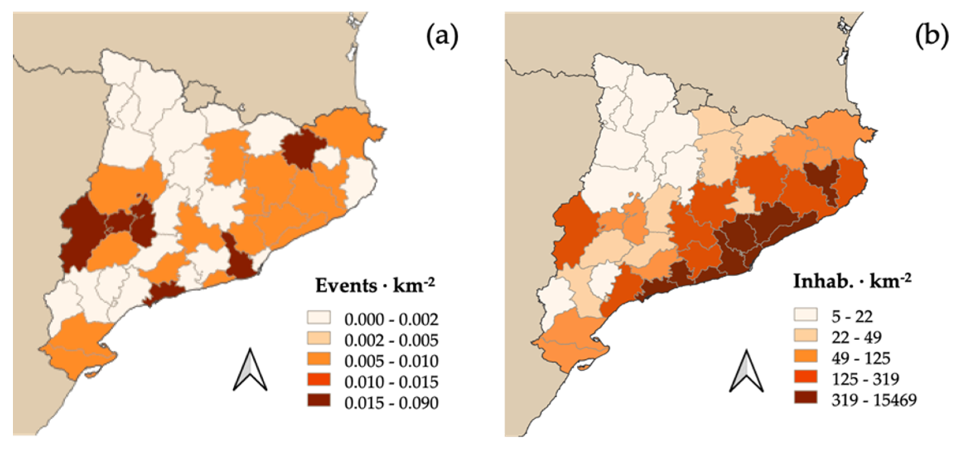
2. Motivation
3. Data and Methods
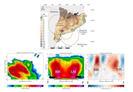
3.1. The XRAD Network and Data
3.2. Dual-Doppler Configuration
3.3. SAMURAI
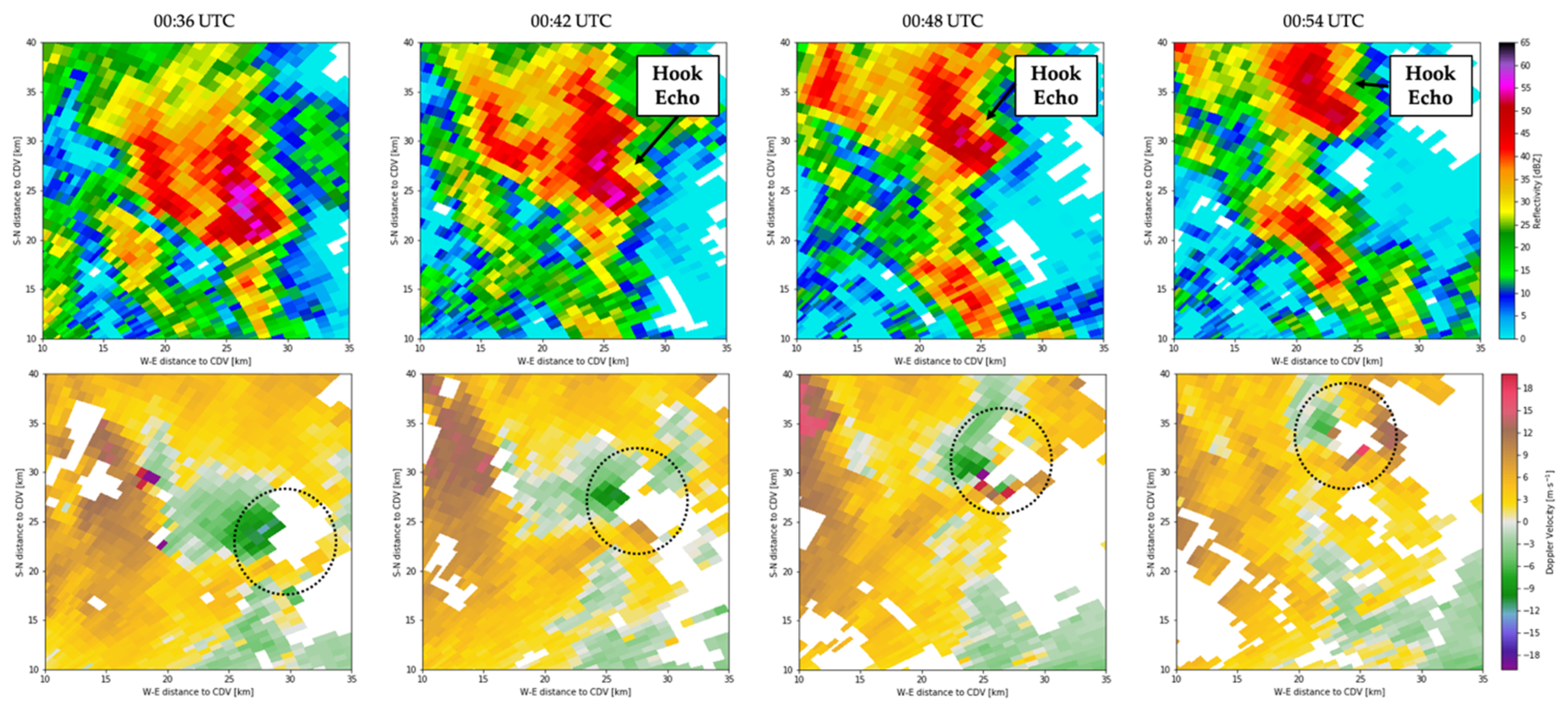
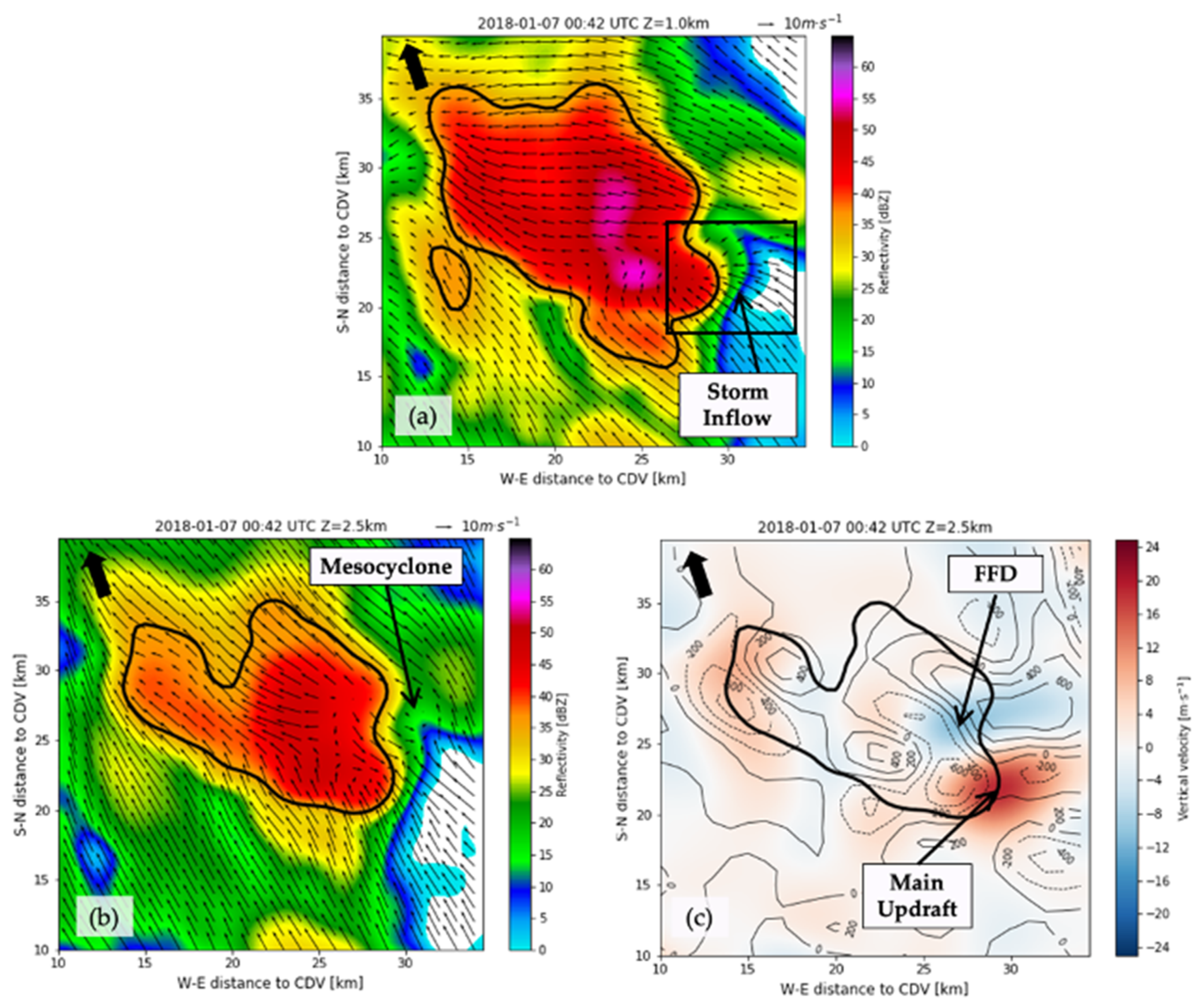
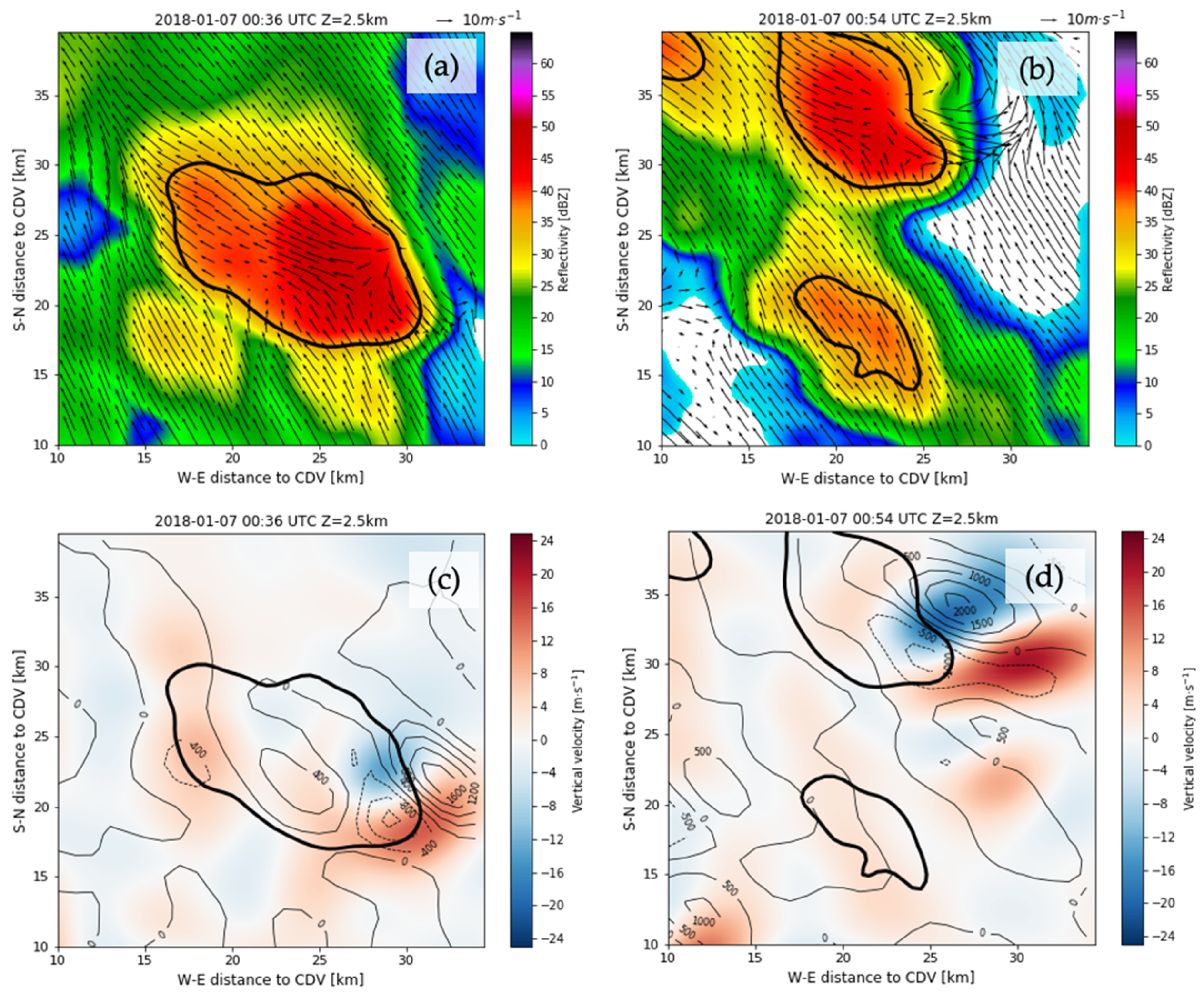
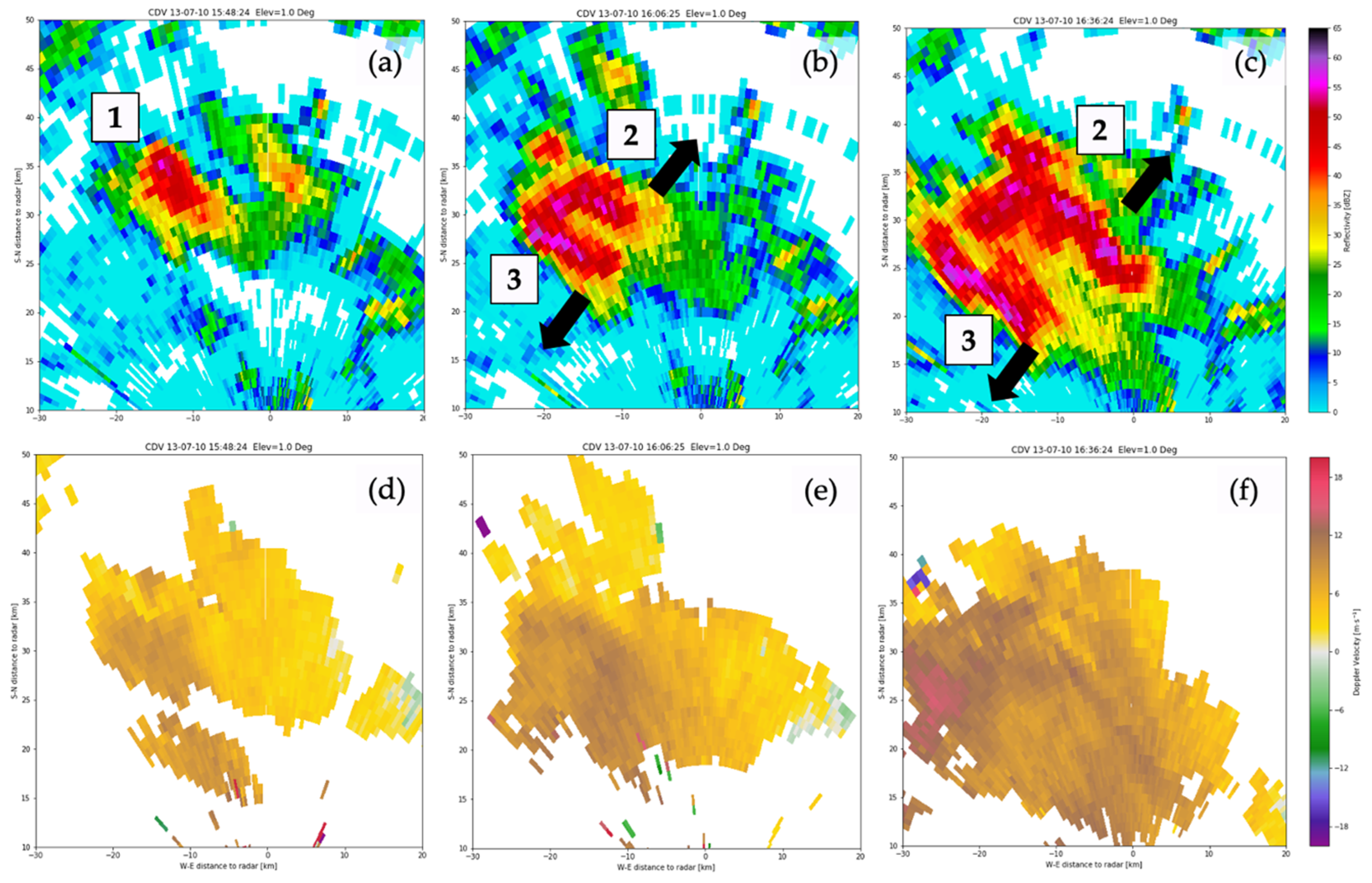
4. Results
4.1. SAMURAI Performance
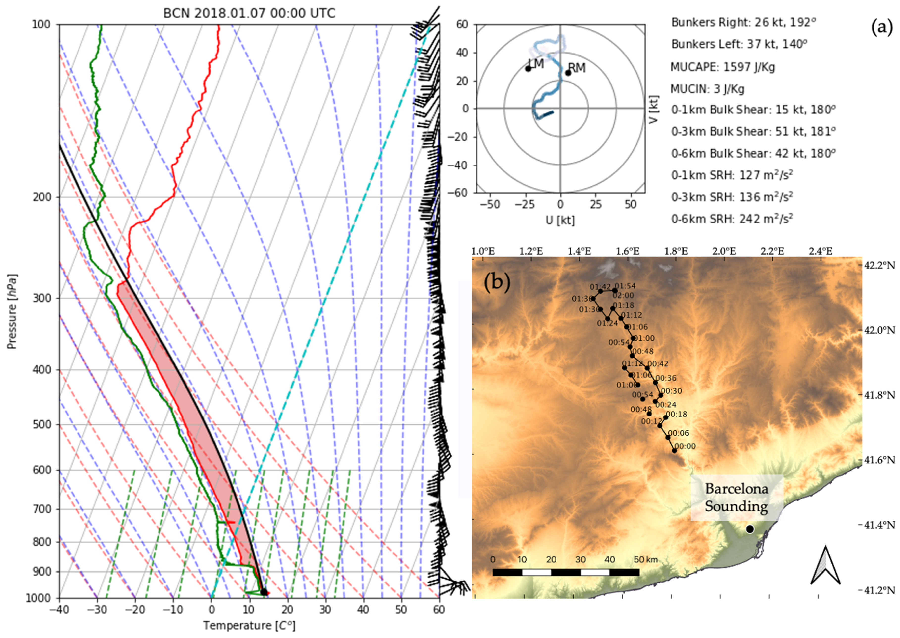
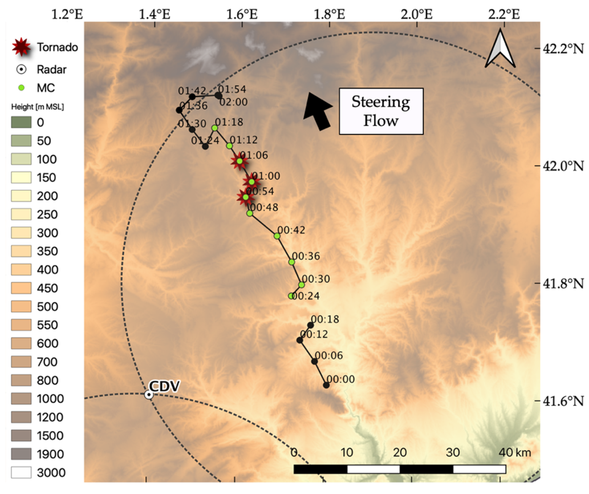
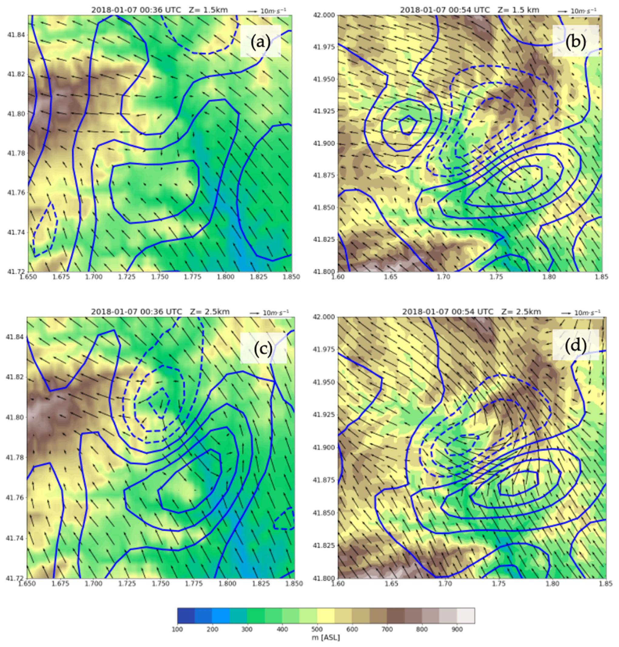
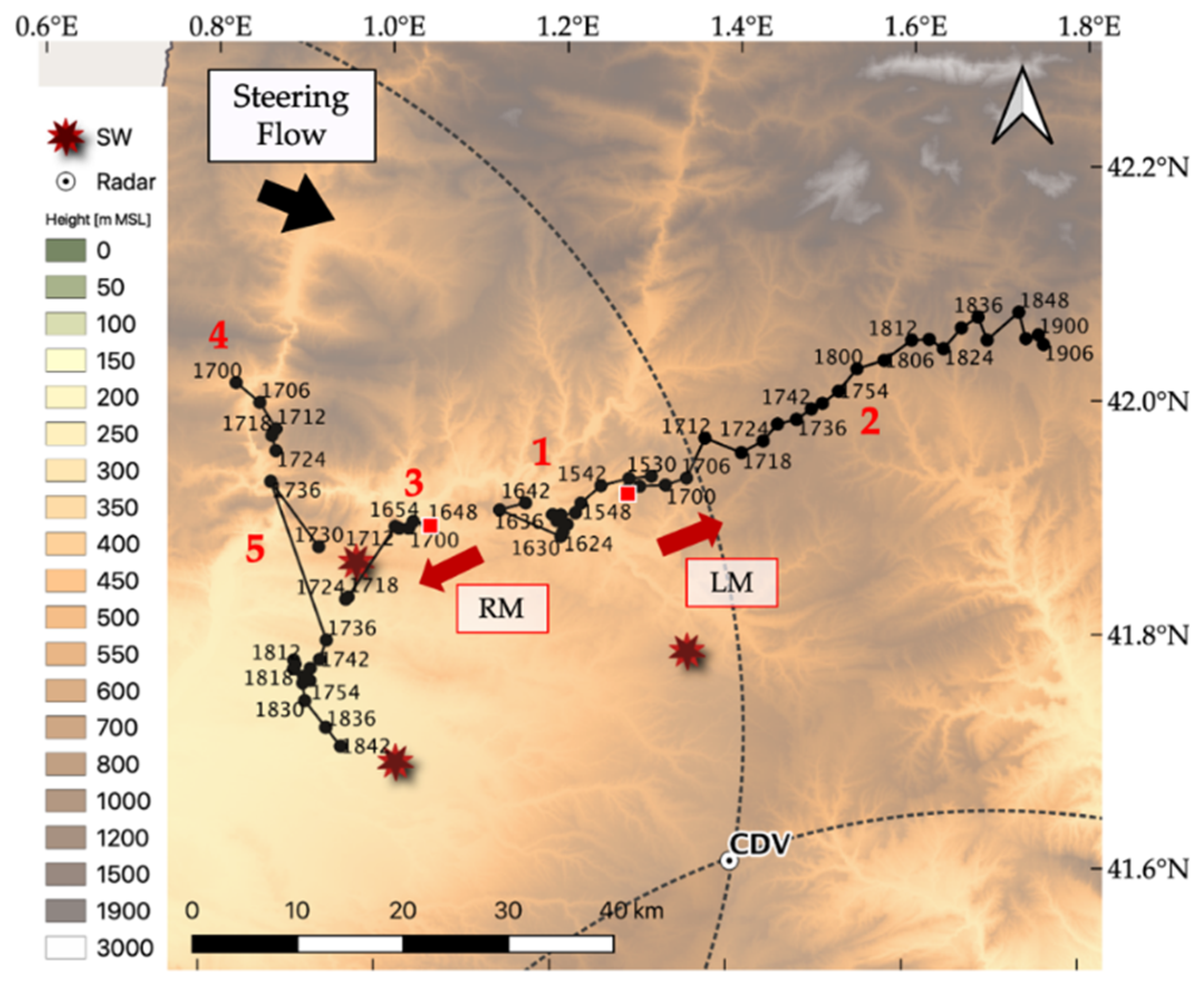
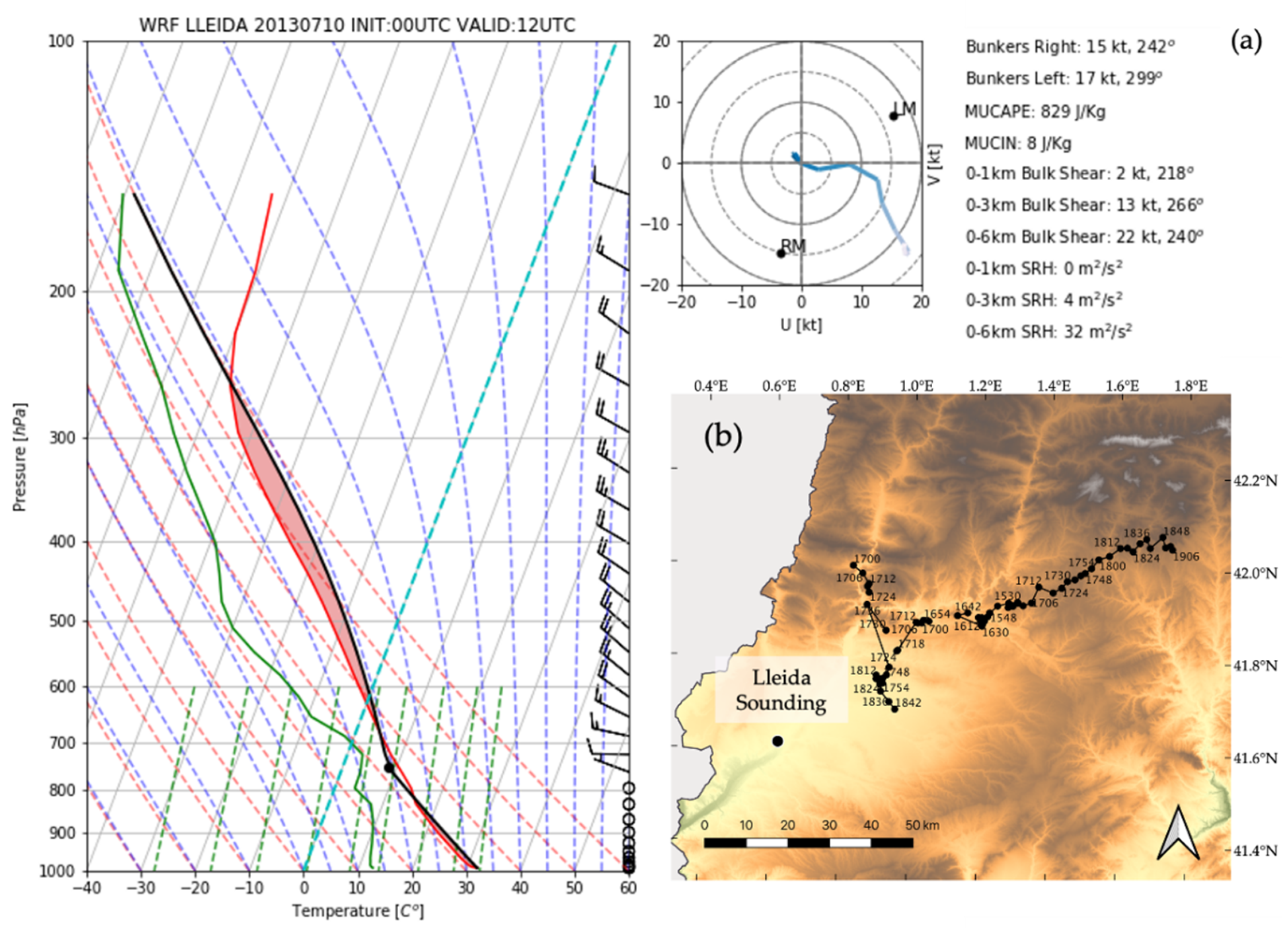
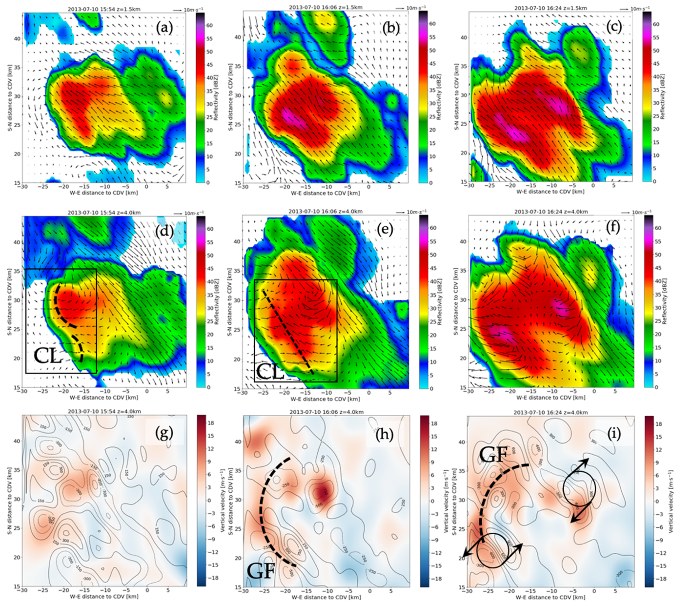
4.2. Dynamical Influence of Topography
5. Discussion and Conclusions
Author Contributions
Funding
Acknowledgments
Conflicts of Interest
References
- Farnell, C.; Rigo, T.; Pineda, N. Lightning jump as a nowcast predictor: Application to severe weather events in Catalonia. Atmos. Res. 2017, 183, 130–141. [Google Scholar] [CrossRef]
- García-Ortega, E.; López, L.; Sánchez, J.L. Atmospheric patterns associated with hailstorm days in the Ebro Valley, Spain. Atmos. Res. 2011, 100, 401–427. [Google Scholar] [CrossRef]
- Rodríguez, O.; Bech, J. Sounding-derived parameters associated with tornadic storms in Catalonia. Int. J. Climatol. 2018, 38, 2400–2414. [Google Scholar] [CrossRef]
- Homar, V.; Gaya, M.; Romero, R.; Ramis, C.; Alonso, S. Tornadoes over complex terrain: An analysis of the 28th August 1999 tornadic event in eastern Spain. Atmos. Res. 2003, 67, 301–317. [Google Scholar] [CrossRef][Green Version]
- del Moral, A.; Llasat, M.C.; Rigo, T. Connecting flash flood events with radar-derived convective storm characteristics on the Northwestern Mediterranean coast: Knowing the present for better future scenarios adaptation. Atmos. Res. 2020, 238, 104–863. [Google Scholar] [CrossRef]
- Rigo, T.; Llasat, M.C. Forecasting hailfall using parameters for convective cells identified by radar. Atmos. Res. 2016, 69, 366–376. [Google Scholar] [CrossRef]
- Klemp, J.B.; Wilhelmson, R.B. The simulation of three-dimensional convective storm dynamics. J. Atmos. Sci. 1978, 35, 1070–1096. [Google Scholar] [CrossRef]
- Rotunno, R.; Ferretti, R. Orographic effects on rainfall in MAP cases IOP 2b and IOP 8. Q. J. R. Meteorol. Soc. A J. Atmos. Sci. Appl. Meteorol. Phys. Oceanogr. 2003, 129, 373–390. [Google Scholar] [CrossRef]
- Armijo, L. A theory for the determination of wind and precipitation velocities with Doppler radars. J. Atmos. Sci. 1969, 26, 570–573. [Google Scholar] [CrossRef]
- Ray, P.S.; Sangren, K.L. Multiple-Doppler radar network design. J. Clim. Appl. Meteorol. 1983, 22, 1444–1454. [Google Scholar] [CrossRef][Green Version]
- Miller, L.J.; Strauch, R.G. A dual Doppler radar method for the determination of wind velocities within precipitating weather systems. Remote Sens. Environ. 1974, 3, 219–235. [Google Scholar] [CrossRef]
- Doviak, R.J.; Ray, P.S.; Strauch, R.G.; Miller, L.J. Error estimation in wind fields derived from dual-Doppler radar measurement. J. Appl. Meteorol. 1976, 15, 868–878. [Google Scholar] [CrossRef]
- Carbone, R.E.; Carpenter, M.J.; Burghart, C.D. Doppler radar sampling limitations in convective storms. J. Atmos. Ocean. Technol. 1985, 2, 357–361. [Google Scholar] [CrossRef][Green Version]
- Shapiro, A.; Potvin, C.K.; Gao, J. Use of a vertical vorticity equation in variational dual-Doppler wind analysis. J. Atmos. Ocean. Technol. 2009, 26, 2089–2106. [Google Scholar] [CrossRef]
- Liou, Y.-C.; Chang, Y.-J. A variational multiple–Doppler radar three-dimensional wind synthesis method and its impacts on thermodynamic retrieval. Mon. Weather Rev. 2009, 137, 3992–4010. [Google Scholar] [CrossRef]
- Potvin, C.K.; Shapiro, A.; Xue, M. Impact of a vertical vorticity constraint in variational dual-doppler wind analysis: Tests with real and simulated supercell data. J. Atmos. Ocean. Technol. 2012, 29, 32–49. [Google Scholar] [CrossRef]
- Gao, J.; Xue, M.; Shapiro, A.; Droegemeier, K.K. A variational method for the analysis of three-dimensional wind fields from two doppler radars. Mon. Wea. Rev. 1999, 127, 2128–2142. [Google Scholar] [CrossRef]
- Liou, Y.; Chang, S.; Sun, J. An application of the immersed boundary method for recovering the three-dimensional wind fields over complex terrain using multiple-doppler radar data. Mon. Wea. Rev. 2012, 140, 1603–1619. [Google Scholar] [CrossRef]
- Dahl, N.A.; Shapiro, A.; Potvin, C.K.; Theisen, A.; Gebauer, J.G.; Schenkman, A.D.; Xue, M. High-Resolution, rapid-scan dual-doppler retrievals of vertical velocity in a simulated supercell. J. Atmos. Ocean. Technol. 2019, 36, 1477–1500. [Google Scholar] [CrossRef]
- Cha, T.Y.; Bell, M.M. Comparison of Single Doppler and Multiple Doppler Wind Retrievals in Hurricane Matthew (2016). Atmos. Meas. Tech. Discuss. 2020, 1–23, in preprint. [Google Scholar]
- Potvin, C.K.; Wicker, L.J.; Shapiro, A. Assessing errors in variational dual-Doppler wind syntheses of supercell thunderstorms observed by storm-scale mobile radars. J. Atmos. Ocean. Technol. 2012, 29, 1009–1025. [Google Scholar] [CrossRef]
- Marquis, J.; Richardson, Y.; Wurman, J.; Markowski, P. Single-and dual-Doppler analysis of a tornadic vortex and surrounding storm-scale flow in the Crowell, Texas, supercell of 30 April 2000. Mon. Weather Rev. 2008, 136, 5017–5043. [Google Scholar] [CrossRef][Green Version]
- Wurman, J.; Kosiba, K.; Markowski, P.; Richardson, Y.; Dowell, D.; Robinson, P. Finescale single-and dual-Doppler analysis of tornado intensification, maintenance, and dissipation in the Orleans, Nebraska, supercell. Mon. Weather Rev. 2010, 138, 4439–4455. [Google Scholar] [CrossRef]
- Kosiba, K.A.; Wurman, J. Finescale dual-Doppler analysis of hurricane boundary layer structures in Hurricane Frances (2004) at landfall. Mon. Weather Rev. 2014, 142, 1874–1891. [Google Scholar] [CrossRef]
- Doviak, R.J.; Zrnic, D.S. Doppler Radar and Weather Observations, 2nd ed.; Dover Publications: New York, NY, USA, 1984; p. 592. [Google Scholar]
- Altube, P.; Bech, J.; Argemí, O.; Rigo, T.; Pineda, N.; Collis, S.; Helmus, J. Correction of dual-PRF doppler velocity outliers in the presence of aliasing. J. Atmos. Ocean. Technol. 2017, 34, 1529–1543. [Google Scholar] [CrossRef]
- Davies-Jones, R.P. Dual-Doppler radar coverage area as a function of measurement accuracy and spatial resolution. J. Appl. Meteorol. 1979, 18, 1229–1233. [Google Scholar] [CrossRef]
- Chong, M.; Georgis, J.-F.; Bousquet, O.; Brodzik, S.R.; Burghart, C.; Cosma, S.; Germann, U.; Gouget, V.; Houze, R.A., Jr.; James, C.N. Real-Time wind synthesis from Doppler radar observations during the Mesoscale Alpine Programme. Bull. Am. Meteorol. Soc. 2000, 81, 2953–2962. [Google Scholar] [CrossRef]
- Bousquet, O.; Chong, M. A multiple-Doppler synthesis and continuity adjustment technique (MUSCAT) to recover wind components from Doppler radar measurements. J. Atmos. Ocean. Technol. 1998, 15, 343–359. [Google Scholar] [CrossRef]
- Bousquet, O.; Tabary, P. Development of a nationwide real-time 3-D wind and reflectivity radar composite in France. Q. J. R. Meteorol. Soc. 2014, 140, 611–625. [Google Scholar] [CrossRef]
- Dolan, B.A.; Rutledge, S.A. An integrated display and analysis methodology for multivariable radar data. J. Appl. Meteorol. Climatol. 2007, 46, 1196–1213. [Google Scholar] [CrossRef]
- Wurman, J. Vector winds from a single-transmitter bistatic dual-Doppler radar network. Bull. Am. Meteorol. Soc. 1994, 75, 983–994. [Google Scholar] [CrossRef][Green Version]
- Friedrich, K.; Hagen, M. On the use of advanced Doppler radar techniques to determine horizontal wind fields for operational weather surveillance. Meteorol. Appl. 2004, 11, 155–171. [Google Scholar] [CrossRef]
- LROSE: Lidar Radar Open Software Environment. Available online: http://lrose.net (accessed on 29 November 2019).
- Aran, M.; Pena, J.; Torà, M. Atmospheric circulation patterns associated with hail events in Lleida (Catalonia). Atmos. Res. 2011, 100, 428–438. [Google Scholar] [CrossRef]
- Bech, J.; Pascual, R.; Rigo, T.; Pineda, N.; López, J.M.; Arús, J.; Gayà, M. An observational study of the 7 September 2005 Barcelona tornado outbreak. Nat. Hazards Earth Syst. Sci. 2007, 7, 129–139. [Google Scholar] [CrossRef][Green Version]
- Rodríguez, O.; Bech, J.; de Dios Soriano, J.; Gutiérrez, D.; Castán, S. A methodology to conduct wind damage field surveys for high-impact weather events of convective origin. Nat. Hazards Earth Syst. Sci. 2020, 20, 1513. [Google Scholar] [CrossRef]
- Tuovinen, J.-P.; Punkka, A.-J.; Rauhala, J.; Hohti, H.; Schultz, D.M. Climatology of severe hail in Finland: 1930–2006. Mon. Weather Rev. 2009, 137, 2238–2249. [Google Scholar] [CrossRef]
- Edwards, R.; Allen, J.T.; Carbin, G.W. Reliability and climatological impacts of convective wind estimations. J. Appl. Meteorol. Climatol. 2018, 57, 1825–1845. [Google Scholar] [CrossRef]
- Skamarock, W.C.; Klemp, J.B.; Dudhia, J.; Gill, D.O.; Barker, D.M.; Duda, M.G.; Huang, X.Y.; Wang, W.; Powers, J.G. G.:A Description of the Advanced Research WRF Version 3; NCAR Tech. Note NCAR/TN-475+ STR; CiteSeerX: State College, PA, USA, 2008; Volume 475. [Google Scholar]
- Mercader, J.; Codina, B.; Sairouni, A.; Cunillera, J. Results of the meteorological model WRF-ARW over Catalonia, using different parameterizations of convection and cloud microphysics. J. Weather Clim. West. Mediterr. 2010, 7, 75–86. [Google Scholar] [CrossRef]
- Cáceres, R.; Codina, B. Radar data assimilation impact over nowcasting a mesoscale convective system in Catalonia using the WRF model. Tethys-J. Mediterr. Meteorol. Climatol. 2018, 15, 3–17. [Google Scholar] [CrossRef]
- del Moral, A.; Rigo, T.; Llasat, M.C. A radar-based centroid tracking algorithm for severe weather surveillance: Identifying split/merge processes in convective systems. Atmos. Res. 2018, 213, 110–120. [Google Scholar] [CrossRef]
- Altube, P.; Bech, J.; Argemí, O.; Rigo, T. Quality control of antenna alignment and receiver calibration using the sun: Adaptation to midrange weather radar observations at low elevation angles. J. Atmos. Ocean. Technol. 2015, 32, 927–942. [Google Scholar] [CrossRef]
- Trapero, L.; Bech, J.; Rigo, T.; Pineda, N.; Forcadell, D. Uncertainty of precipitation estimates in convective events by the Meteorological Service of Catalonia radar network. Atmos. Res. 2009, 93, 408–418. [Google Scholar] [CrossRef]
- Vaisala USER’S MANUAL: Digital IF Receiver/Doppler Signal Processor, RVP8 (M211321EN-B); Vaisala: Vantaa, Finland, 2014; p. 524.
- Dazhang, T. Evaluation of alternative-PRF method for extending the range of unambiguous Doppler velocity. In Proceedings of the 22nd Conference on Radar Meteor, Zurich, Switzerland, 10–13 September 1984; pp. 523–527. [Google Scholar]
- May, P.T. Mesocyclone and microburst signature distortion with dual PRT radars. J. Atmos. Ocean. Technol. 2001, 18, 1229–1233. [Google Scholar] [CrossRef]
- Oye, R.; Mueller, C.; Smith, S. Software for radar translation, visualization, editing, and interpolation. In Proceedings of the Preprints, 27th Conference on Radar Meteorology, Vail, CO, USA, 9–13 October 1995; pp. 359–361. [Google Scholar]
- Lhermitte, R.M.; Miller, L.J. Doppler Radar Methodology for Observation of Convective Storms. In Proceedings of the 14th Conference on Radar Meteorology, Tucson, AR, USA, 17–20 November 1970; Bulleting of the American Meteorological Society. Volume 51, p. 772. [Google Scholar]
- Bell, M.M.; Montgomery, M.T.; Emanuel, K.A. Air–Sea enthalpy and momentum exchange at major hurricane wind speeds observed during CBLAST. J. Atmos. Sci. 2012, 69, 3197–3222. [Google Scholar] [CrossRef]
- Ooyama, K.V. Scale-Controlled objective analysis. Mon. Weather Rev. 1987, 115, 2479–2506. [Google Scholar] [CrossRef][Green Version]
- Ooyama, K.V. The cubic-spline transform method: Basic definitions and tests in a 1D single domain. Mon. Weather Rev. 2002, 130, 2392–2415. [Google Scholar] [CrossRef]
- Foerster, A.M.; Bell, M.M.; Harr, P.A.; Jones, S.C. Observations of the eyewall structure of Typhoon Sinlaku (2008) during the transformation stage of extratropical transition. Mon. Weather Rev. 2014, 142, 3372–3392. [Google Scholar] [CrossRef][Green Version]
- Foerster, A.M.; Bell, M.M. Thermodynamic retrieval in rapidly rotating vortices from multiple-Doppler radar data. J. Atmos. Ocean. Technol. 2017, 34, 2353–2374. [Google Scholar] [CrossRef]
- Gao, J.; Xue, M.; Brewster, K.; Droegemeier, K.K. A three-dimensional variational data analysis method with recursive filter for Doppler radars. J. Atmos. Ocean. Technol. 2004, 21, 457–469. [Google Scholar] [CrossRef]
- Purser, R.J.; Wu, W.-S.; Parrish, D.F.; Roberts, N.M. Numerical aspects of the application of recursive filters to variational statistical analysis. Part I: Spatially homogeneous and isotropic Gaussian covariances. Mon. Weather Rev. 2003, 131, 1524–1535. [Google Scholar] [CrossRef]
- Dixon, M.J.; Lee, W.-C.; Rilling, R.A.; Burghart, C.D.; Van Andel, J.H. CfRadial Data File Format: Proposed CF-Compliant netCDF Format for Moments Data for RADAR and LIDAR in Radial Coordinates. 2013. Available online: http://n2t.net/ark:/85065/d7ff3rbc (accessed on 21 April 2020).
- Farnell, C.; Rigo, T. The Lightning Jump, the 2018 “Picking up Hailstones” Campaign and a Climatological Analysis for Catalonia for the 2006–2018 Period. Tethys 2020, 17, 10–20. [Google Scholar]
- McDonald, J.R.; Mehta, K.C.; Smith, D.A.; Womble, J.A. The enhanced fujita scale: Development and implementation. In Forensic Engineering 2009: Pathology of the Built Environment; American Society of Civil Engineers: Reston, VA, USA, 2010; pp. 719–728. [Google Scholar]
- Bluestein, H.B.; Parker, S.S. Modes of isolated, severe convective storm formation along the dryline. Mon. Weather Rev. 1993, 121, 1354–1372. [Google Scholar] [CrossRef]
- Bunkers, M.J.; Klimowski, B.A.; Zeitler, J.W.; Thompson, R.L.; Weisman, M.L. Predicting supercell motion using a new hodograph technique. Weather Forecast. 2000, 15, 61–79. [Google Scholar] [CrossRef]
- May, R.M.; Arms, S.C.; Marsh, P.; Bruning, E.; M Leeman, J.R.; Goebbert, K.; Thielen, J.E.; Bruick, Z. MetPy: A Python Package for Meteorological Data. 2020. Available online: https://github.com/Unidata/MetPy (accessed on 21 April 2020). [CrossRef]
- Lemon, L.R.; Doswell, C.A., III. Severe thunderstorm evolution and mesocyclone structure as related to tornadogenesis. Mon. Weather Rev. 1979, 107, 1184–1197. [Google Scholar] [CrossRef]
- Markowski, P.; Richardson, Y. Mesoscale Meteorology in Midlatitudes; John Wiley and Sons: West Sussex, UK, 2011; Volume 2. [Google Scholar]
- Doswell, C.A., III. Seeing supercells as heavy rain producers. In Proceedings of the Preprints, 14th Conference on Hydrology, Dallas, TX, USA, 10–15 January 1998; Amer. Meteor. Soc. pp. 73–76. [Google Scholar]
- Johns, R.H.; Davies, J.M.; Leftwich, P.W. Some wind and instability parameters associated with strong and violent tornadoes: 2. Variations in the combinations of wind and instability parameters. GMS 1993, 79, 583–590. [Google Scholar]
- Carbunaru, D.; Stefan, S.; Sasu, M.; Stefanescu, V. Analysis of convective thunderstorm split cells in south-eastern Romania. Int. J. Atmos. Sci. 2013, 2013, 19–38. [Google Scholar] [CrossRef]
- Weisman, M.L.; Rotunno, R. The use of vertical wind shear versus helicity in interpreting supercell dynamics. J. Atmos. Sci. 2000, 57, 1452–1472. [Google Scholar] [CrossRef]
- Clark, A.J.; Schaffer, C.J.; Gallus, W.A., Jr.; Johnson-O’Mara, K. Climatology of storm reports relative to upper-level jet streaks. Weather Forecast. 2009, 24, 1032–1051. [Google Scholar] [CrossRef]
- Bousquet, O.; Tabary, P.; Parent du Châtelet, J. Operational multiple-Doppler wind retrieval inferred from long-range radial velocity measurements. J. Appl. Meteor. Climatol. 2008, 47, 2929–2945. [Google Scholar] [CrossRef]
- Collis, S.; Protat, A.; Chung, K.-S. The effect of radial velocity gridding artifacts on variationally retrieved vertical velocities. J. Atmos. Ocean. Tech. 2010, 27, 1239–1246. [Google Scholar] [CrossRef]
- Oue, M.; Kollias, P.; Shapiro, A.; Tatarevic, A.; Matsui, T. Investigation of observational error sources in multi-Doppler-radar three-dimensional variational vertical air motion retrievals. Atmos. Meas. Tech. 2019, 12, 1999–2018. [Google Scholar] [CrossRef]
- Liou, Y.; Bluestein, H.B.; French, M.M.; Wienhoff, Z.B. Single-Doppler velocity retrieval of the wind field in a tornadic supercell using mobile, phased-array, doppler radar data. J. Atmos. Ocean. Technol. 2018, 35, 1649–1663. [Google Scholar] [CrossRef]
- Miller, L.J.; Fredrick, S.M. Custom Editing and Display of Reduced Information in Cartesian Space (CEDRIC) Manual; National Center for Atmospheric Research, Mesoscale and Microscale Meteorology Division: Boulder, CO, USA, 1998; Volume 130.
- Seneviratne, S.I.; Nicholls, N.; Easterling, D.; Goodess, C.M.; Kanae, S.; Kossin, J.; Luo, Y.; Marengo, J.; McInnes, K.; Rahimi, M.; et al. Changes in climate extremes and their impacts on the natural physical environment. In Managing the Risks of Extreme Events and Disasters to Advance Climate Change Adaptation. A Special Report of Working Groups I and II of the Intergovernmental Panel on Climate Change (IPCC); Cambridge University Press: Cambridge, UK; New York, NY, USA, 2012; pp. 109–230. [Google Scholar]
- Cramer, W.; Guiot, J.; Fader, M.; Garrabou, J.; Gattuso, J.-P.; Iglesias, A.; Lange, M.A.; Lionello, P.; Llasat, M.C.; Paz, S. Climate change and interconnected risks to sustainable development in the Mediterranean. Nat. Clim. Chang. 2018, 8, 972–980. [Google Scholar] [CrossRef]


| Radar | Abbrev | Height (m ASL) | Lat, Lon (°) | Ranges (km) | Elev. (°)/num. | Radar Gate Spacing (m) |
|---|---|---|---|---|---|---|
| Puig Bernat | PBE | 610 | 41.37, 1.39 | 130–240 | 0.6–27/16 | 250 |
| Puig d’Arques | PDA | 542 | 41.89, 2.99 | 130–240 | 0.6–27/16 | 250 |
| Creu del Vent | CDV | 825 | 41.96, 1.40 | 150–250 | 0.6–27/16 | 250 |
| La Miranda | LMI | 910 | 41.09, 0.86 | 130–240 | 0.6–27/16 | 250 |
| Radar Pair | Baseline (km) | Farthest Point (km) | Resolution (km) | Total Area (103km2) | Optimal Area (103km2) | Blockage (%) |
|---|---|---|---|---|---|---|
| CDV-PBE | 47.33 | 94.66 | 1.98 | 13.30 | 10.34 | 1.48 |
| CDV-LMI | 72.60 | 145.20 | 3.04 | 31.04 | 7.99 | 1.68 |
| PBE-LMI | 90.83 | 181.66 | 3.80 | 49.02 | 5.12 | 3.01 |
| PBE-PDA | 109.01 | 218.02 | 4.57 | 70.78 | 2.82 | 0.00 |
| CDV-PDA | 136.10 | 272.20 | 5.70 | 110.30 | 0.58 | 0.00 |
| Z Radius Infl. (km) | Gaussian Filter (Δ) | Spline Cutoff (Δ) | Analysis Grid Increment (km) |
|---|---|---|---|
| 1 | 4; 4; 2 | 2; 2; 2 | 0.5; 0.5; 0.5 |
© 2020 by the authors. Licensee MDPI, Basel, Switzerland. This article is an open access article distributed under the terms and conditions of the Creative Commons Attribution (CC BY) license (http://creativecommons.org/licenses/by/4.0/).
Share and Cite
del Moral, A.; Weckwerth, T.M.; Rigo, T.; Bell, M.M.; Llasat, M.C. C-Band Dual-Doppler Retrievals in Complex Terrain: Improving the Knowledge of Severe Storm Dynamics in Catalonia. Remote Sens. 2020, 12, 2930. https://doi.org/10.3390/rs12182930
del Moral A, Weckwerth TM, Rigo T, Bell MM, Llasat MC. C-Band Dual-Doppler Retrievals in Complex Terrain: Improving the Knowledge of Severe Storm Dynamics in Catalonia. Remote Sensing. 2020; 12(18):2930. https://doi.org/10.3390/rs12182930
Chicago/Turabian Styledel Moral, Anna, Tammy M. Weckwerth, Tomeu Rigo, Michael M. Bell, and María Carmen Llasat. 2020. "C-Band Dual-Doppler Retrievals in Complex Terrain: Improving the Knowledge of Severe Storm Dynamics in Catalonia" Remote Sensing 12, no. 18: 2930. https://doi.org/10.3390/rs12182930
APA Styledel Moral, A., Weckwerth, T. M., Rigo, T., Bell, M. M., & Llasat, M. C. (2020). C-Band Dual-Doppler Retrievals in Complex Terrain: Improving the Knowledge of Severe Storm Dynamics in Catalonia. Remote Sensing, 12(18), 2930. https://doi.org/10.3390/rs12182930