Ground-Based Radar Interferometry for Monitoring the Dynamic Performance of a Multitrack Steel Truss High-Speed Railway Bridge

 ,
,  ,
, 

Abstract
1. Introduction
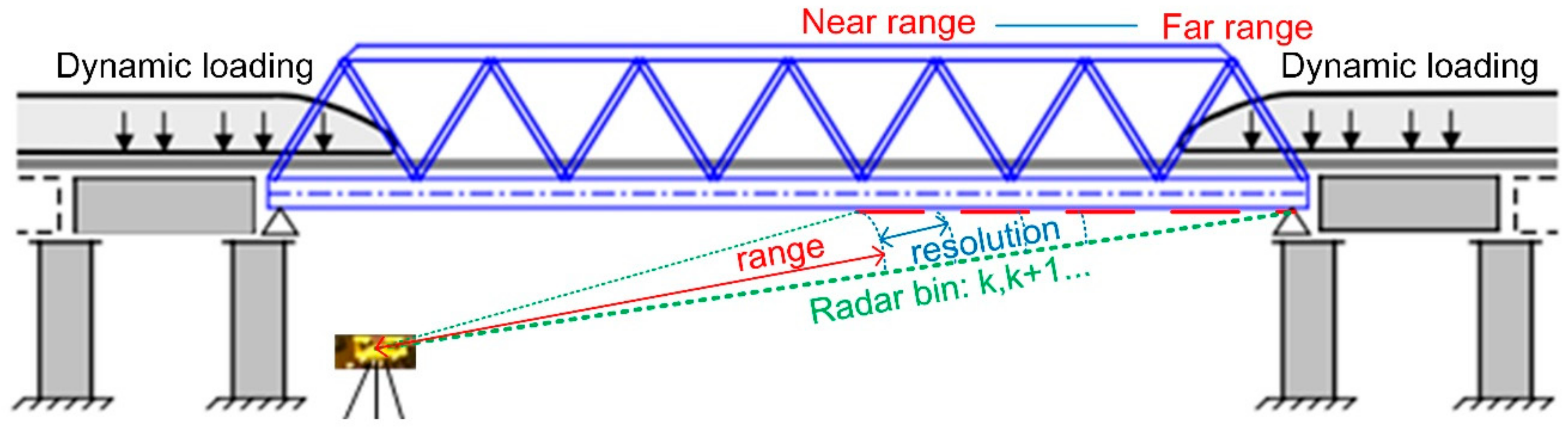
2. Ground-Based Interferometric Radar
3. Bridge Description and Experimental Setting
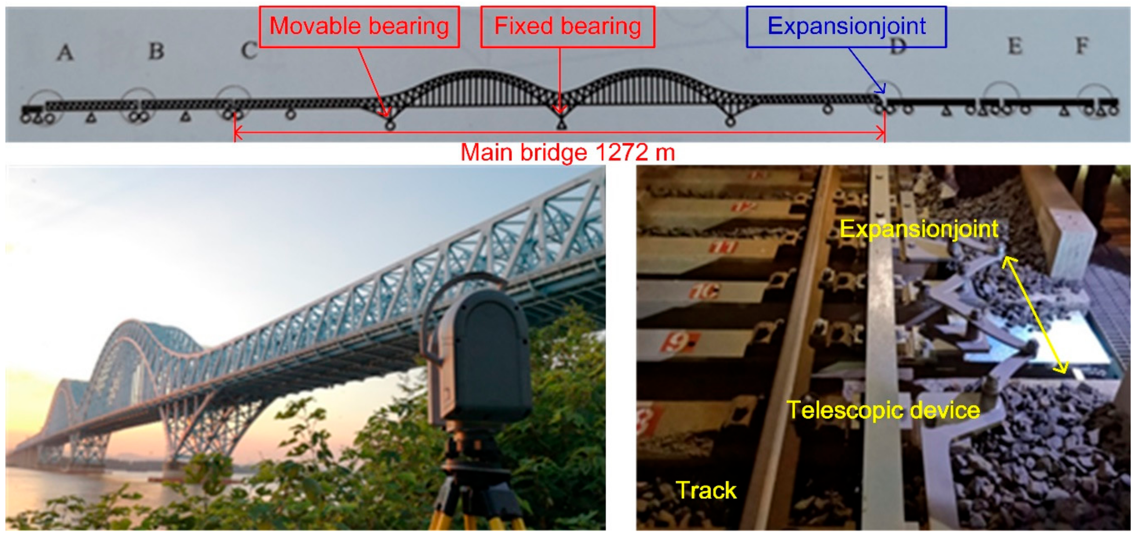
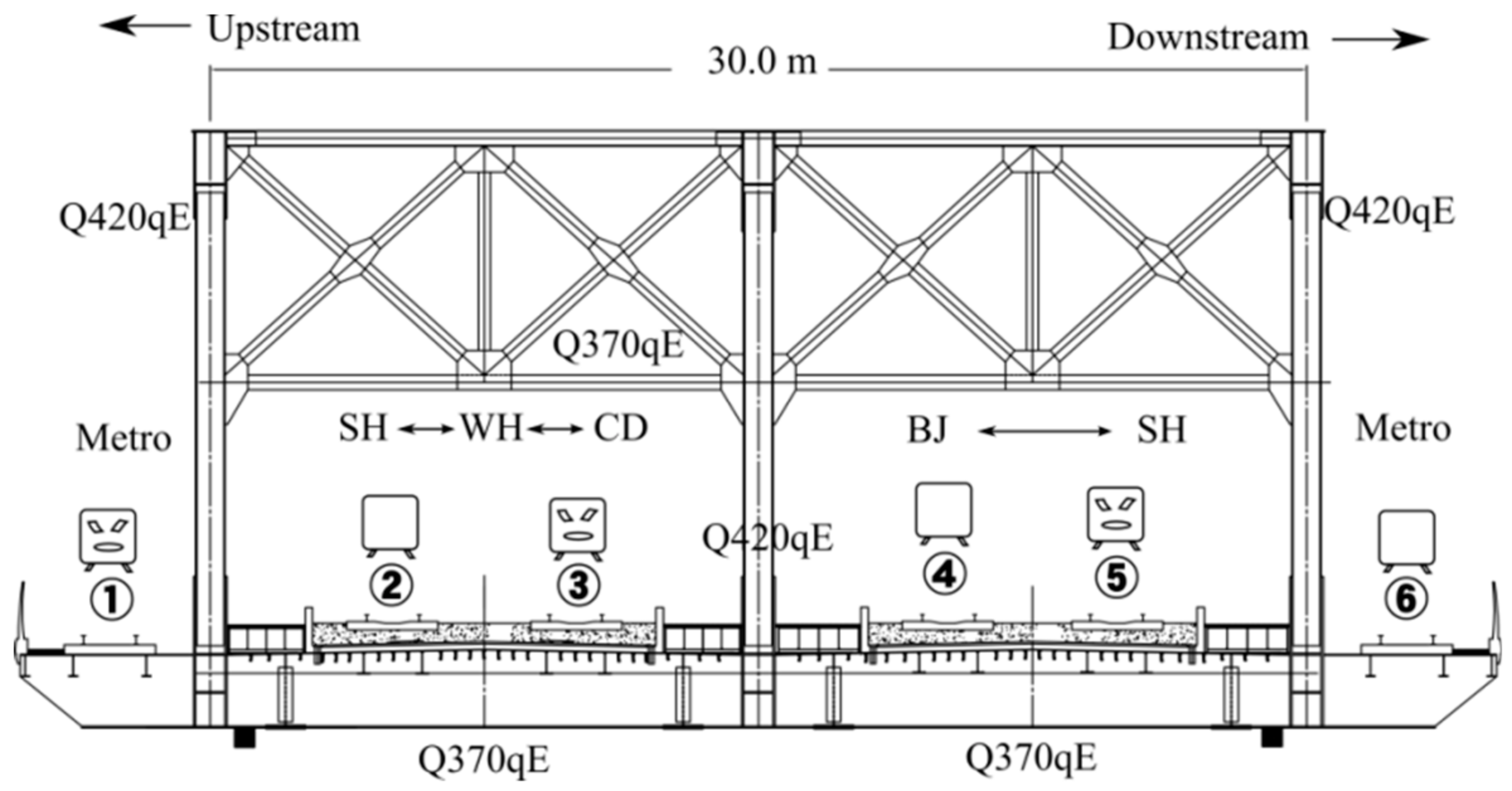
3.1. Bridge Description
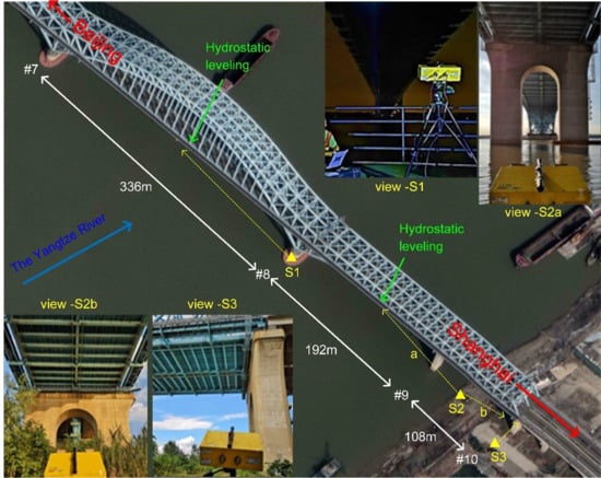
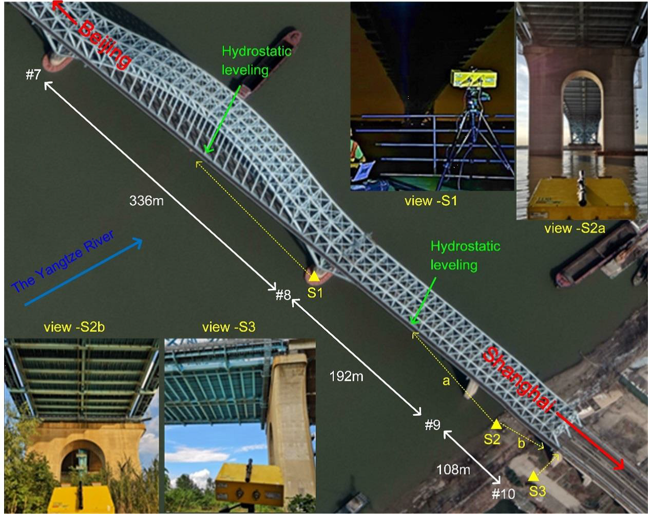
3.2. Experimental Settings
4. Results of the Bridge Dynamic Responses
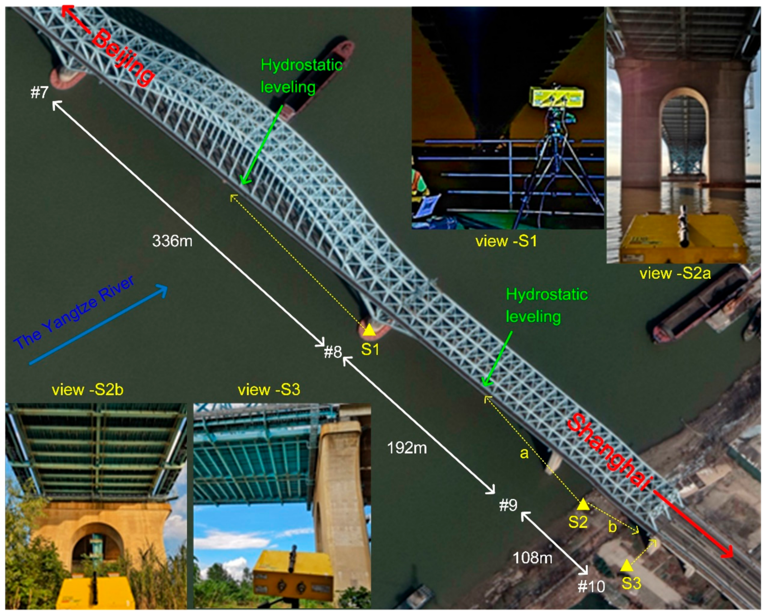
4.1. Ambient Vibration of the 336-m Span
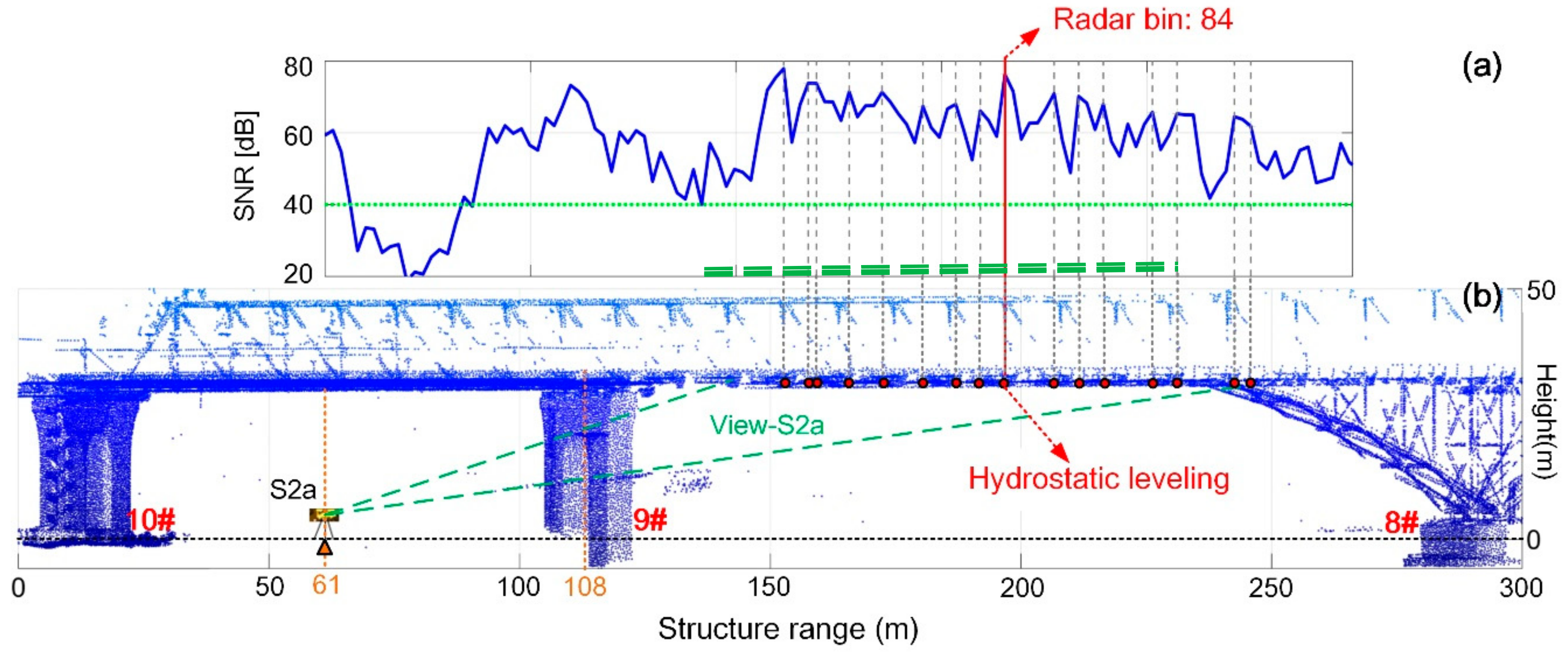
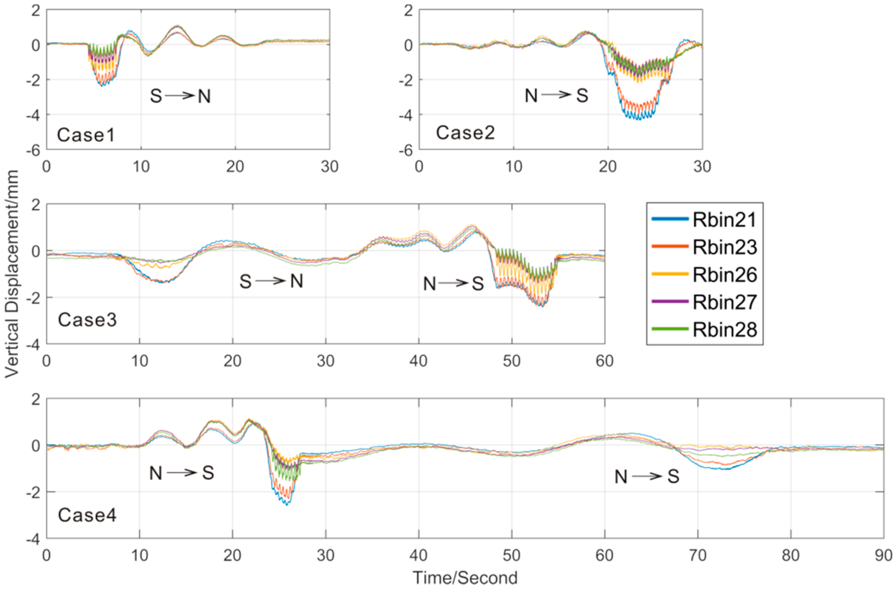
4.2. Dynamic Vibration of the 192-m Span
- (1)
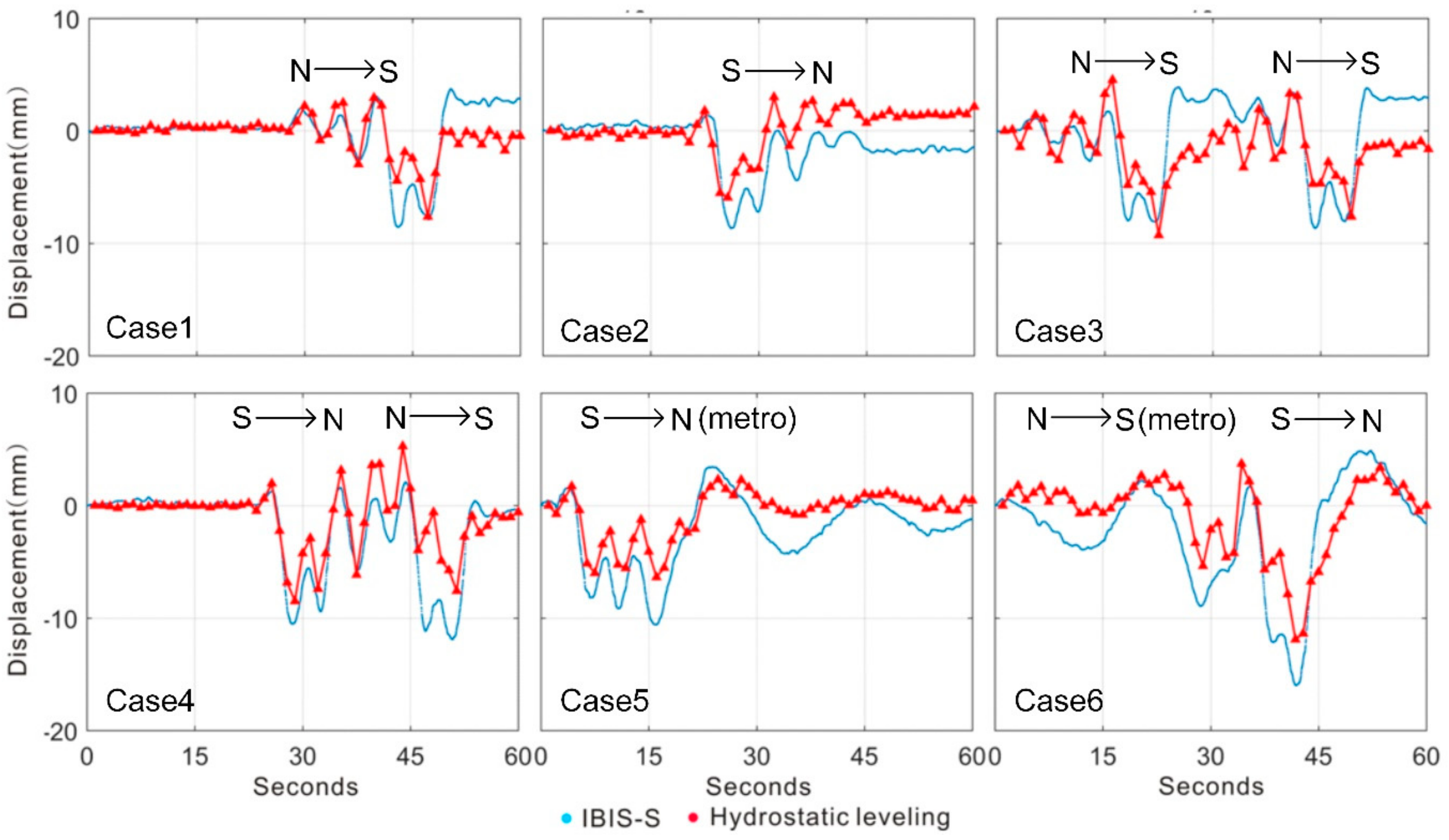
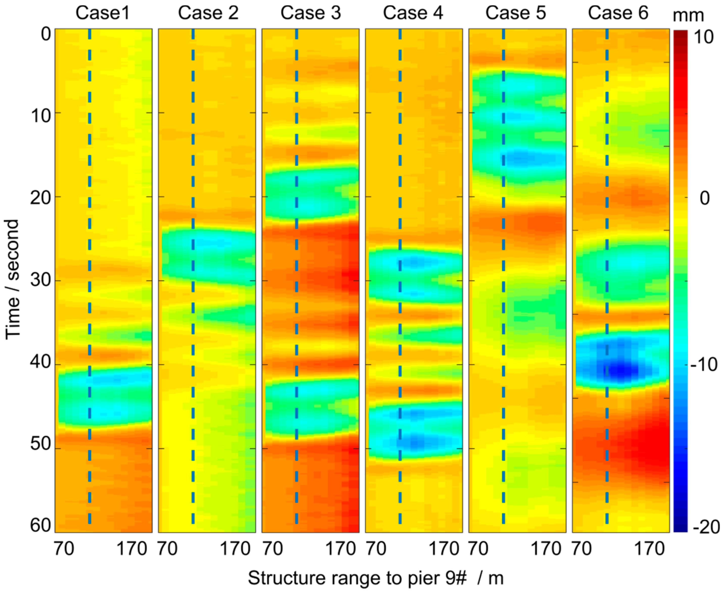
- As far as the train-induced displacement procedures are considered, the radar and hydrostatic leveling results are quite consistent in the six different load cases;
- (2)
- The hydrostatic leveling results about the train-induced displacements miss the real peak in most instances. By contrast, the radar results provide a higher detail in the description of the displacement behavior. This is due to the higher sampling frequency (53.845 Hz) with respect to leveling sensor (1 Hz). This can help the engineers to capture the maximum value of the train-induced displacements of bridge;
- (3)
- The displacements occur as soon as the given train reaches the main bridge, and they decrease to the normal state as far as the loading disappears. This is evident by calculating the duration of the loading on the main bridge. For instance, in Case 1 the displacement lasts for about 25 s. Considering the velocity of the train (237.7 km/h), the main bridge length (1272 m) and the train length (400 m, 16 carriages of 25 m each), the total time for the train passing the bridge is about 25.3 s. The same result can be achieved for the metro, considering the 6 carriages of 20 m each, with a speed of about 80 km/h;
- (4)
- The temporal evolution of the displacements is related to the direction of the passing train. When the train arrives, small displacements are detected at the beginning; then they transmit like a sine wave, while the displacement amplitude becomes larger and larger; when the train leaves the bridge, the displacements disappear quickly. The behavior is symmetric for the trains coming from north to south (N2S) and from south to north (S2N);
- (5)
- The vertical displacements achieve the maximum value when the train is running on the measuring point. In all cases, the displacement magnitude is less than 12 mm;
- (6)
- The magnitude of vertical displacement, as well as the duration, does not significantly increase when two trains are running simultaneously on the bridge. This is in agreement with the structural characteristic of NDHRB, which is a rigid bridge.
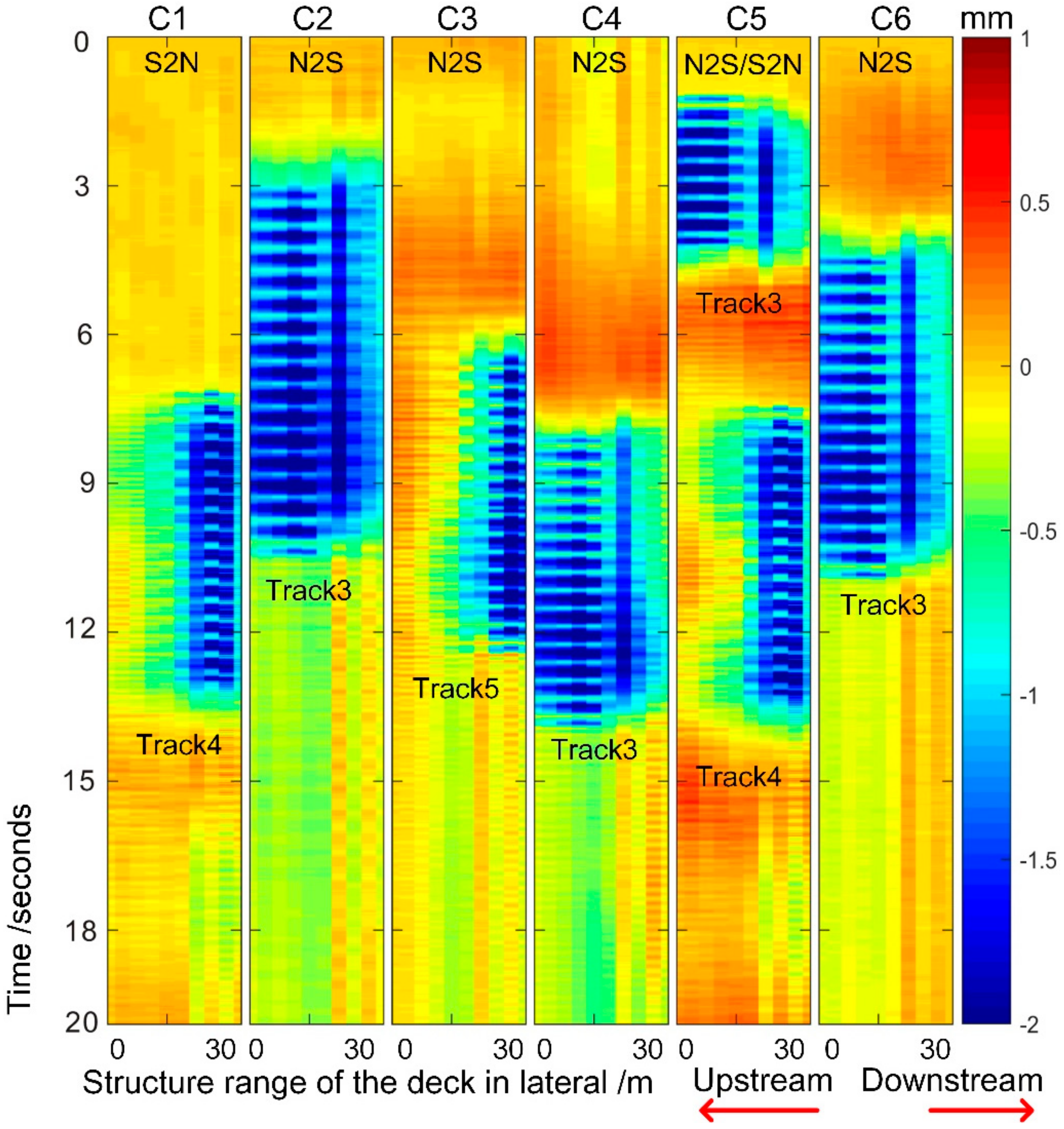
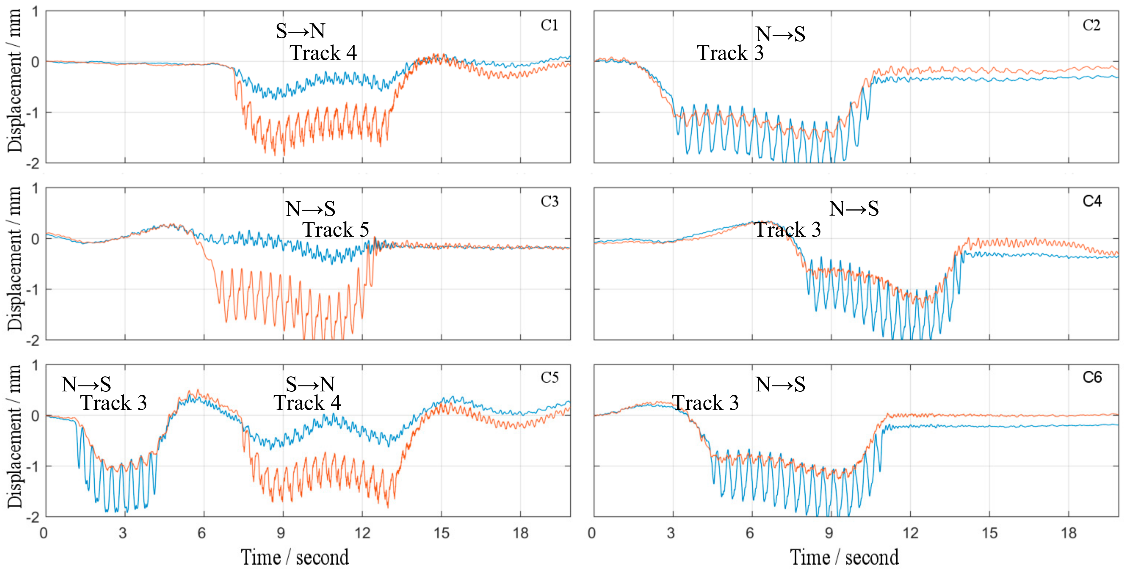
4.3. Dynamic Behavior at the Expansion Joints
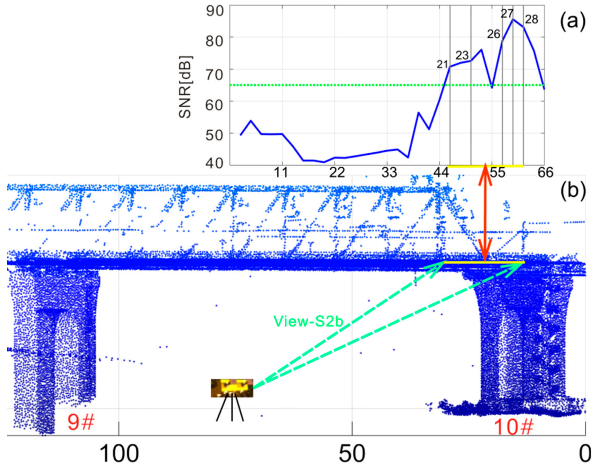
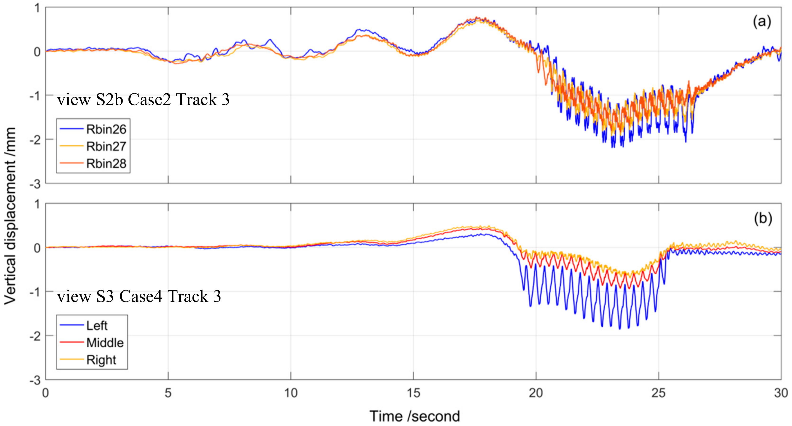
4.3.1. View-S2b and Results
4.3.2. View S3 and Results
5. Discussion
6. Conclusions
- (1)
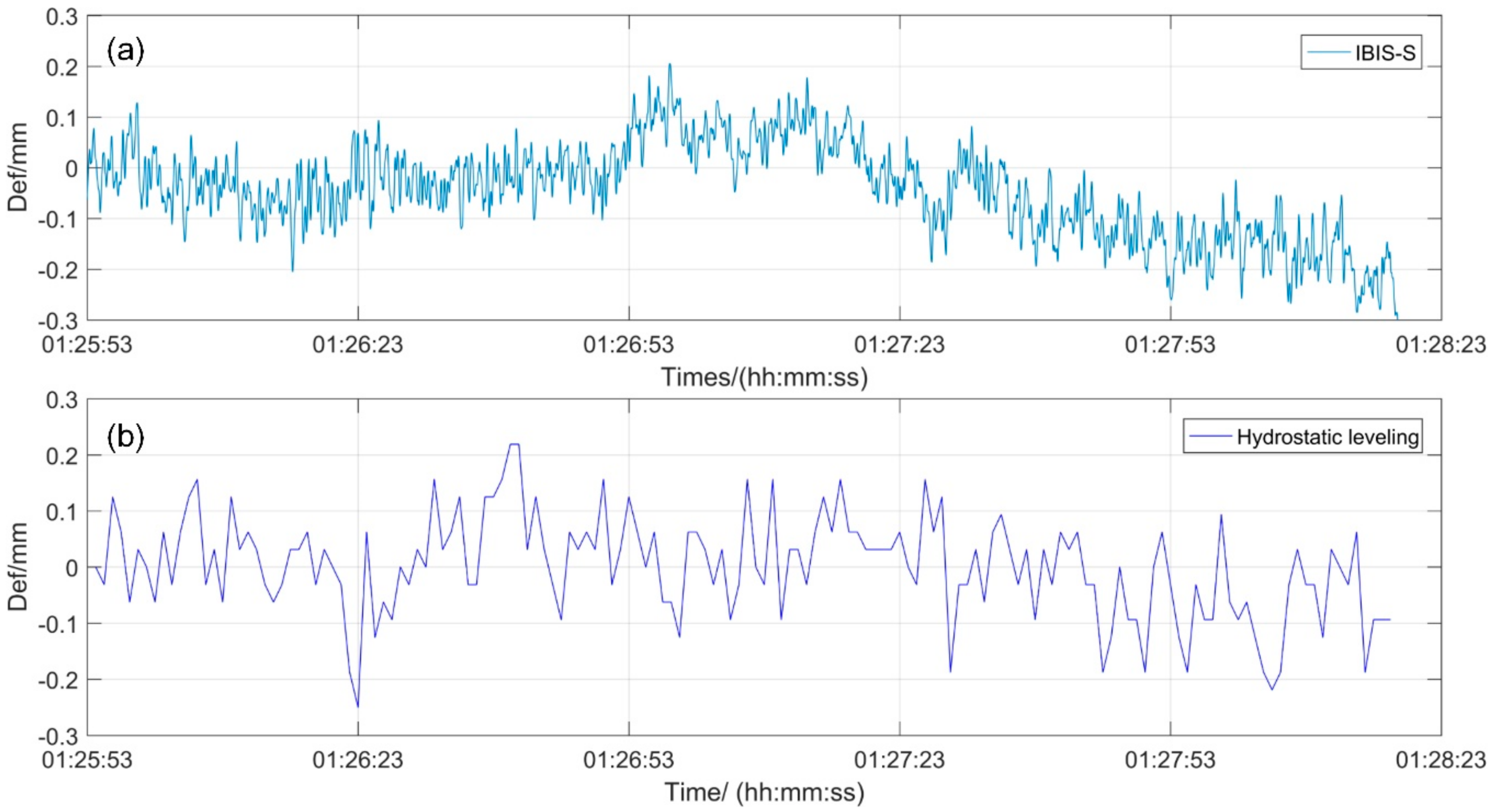
- The radar measurements at S1 show that, for a 336-m steel truss span, the magnitude of ambient vibration in the bridge vertical is within ±0.3 mm. This response agrees with the rigid characteristic of the railway bridge at hand;
- (2)
- The experimental results at S2 show that, for a 192-m steel truss span, the vertical displacements induced by high speed passing train (250 km/h) are less than 12 mm; the pattern of the displacement time history is related to the track of train and its duration depends on the period during which the train is passing on the main bridge. Good consistency in all the representative loading cases was achieved with the in-situ SHM system data. A more detailed displacement behavior is achieved from IBIS-S due to its higher sampling frequency and the maximum displacements are captured;
- (3)
- The lateral behavior of the bridge can be studied when setting the radar perpendicularly to the bridge, while the traditional way of sensor setting (parallel to the bridge) cannot. Measurements of the bridge deck perpendicularly to the bridge (S3) show that, for a multitrack steel truss bridge, the vertical displacements are not uniform in bridge lateral direction larger displacements are monitored in the track where the train is passing, while minor effects are present on other tracks.
Author Contributions
Funding
Acknowledgments
Conflicts of Interest
References
- Zhao, H.; Ding, Y.; Nagarajaiah, S.; Li, A. Behavior Analysis and Early Warning of Girder Deflections of a Steel-Truss Arch Railway Bridge under the Effects of Temperature and Trains: Case Study. J. Bridge Eng. 2019, 24. [Google Scholar] [CrossRef]
- Ding, Y.; Wang, G.; Sun, P.; Wu, L.; Yue, Q. Long-Term Structural Health Monitoring System for a High-Speed Railway Bridge Structure. Sci. World J. 2015, 2015, 250562. [Google Scholar] [CrossRef] [PubMed]
- Wang, H.; Chang, L.; Markine, V. Structural Health Monitoring of Railway Transition Zones Using Satellite Radar Data. Sensors 2018, 18, 413. [Google Scholar] [CrossRef]
- Huang, Q.; Crosetto, M.; Monserrat, O.; Crippa, B. Displacement monitoring and modelling of a high-speed railway bridge using C-band Sentinel-1 data. ISPRS J. Photogramm. Remote Sens. 2017, 128, 204–211. [Google Scholar] [CrossRef]
- Huang, Q.; Monserrat, O.; Crosetto, M.; Crippa, B.; Wang, Y.; Jiang, J.; Ding, Y. Displacement Monitoring and Health Evaluation of Two Bridges Using Sentinel-1 SAR Images. Remote Sens. 2018, 10, 1714. [Google Scholar] [CrossRef]
- Cosser, E.; Roberts, G.W.; Meng, X.; Dodson, A.H. Measuring the dynamic deformation of bridges using a total station. In Proceedings of the 11th FIG Symposium on Deformation Measurements, Santorini, Greece, 25–28 May 2003. [Google Scholar]
- De Battista, N.; Westgate, R.; Koo, K.Y.; Brownjohn, J. Wireless monitoring of the longitudinal displacement of the Tamar Suspension Bridge deck under changing environmental conditions. In Proceedings of the SPIE—The International Society for Optical Engineering, San Diego, CA, USA, 7–10 March 2011; Tomizuka, M., Yun, C.B., Giurgiutiu, V., Lynch, J.P., Eds.; Spie-Int Soc Optical Engineering: Bellingham, WA, USA, 2011; Volume 7981. [Google Scholar]
- Meng, X.; Roberts, G.W.; Dodson, A.H.; Cosser, E.; Barnes, J.; Rizos, C. Impact of GPS satellite and pseudolite geometry on structural deformation monitoring: Analytical and empirical studies. J. Geod. 2004, 77, 809–822. [Google Scholar] [CrossRef]
- Park, K.; Hwang, E. Assessment of vibration serviceability for steel cable-stayed bridges using GNSS data. Int. J. Steel Struct. 2016, 16, 1251–1262. [Google Scholar] [CrossRef]
- Dai, D.; Wang, X.; Zhan, D.; Qin, S.; Huang, Z. Dynamic measurement of high-frequency deflections of the vertical based on the observation of INS/GNSS integration attitude error. J. Appl. Geophys. 2015, 119, 89–98. [Google Scholar] [CrossRef]
- Ribeiro, D.; Calçada, R.; Ferreira, J.; Martins, T. Non-contact measurement of the dynamic displacement of railway bridges using an advanced video-based system. Eng. Struct. 2014, 75, 164–180. [Google Scholar] [CrossRef]
- Nassif, H.H.; Gindy, M.; Davis, J. Comparison of laser Doppler vibrometer with contact sensors for monitoring bridge deflection and vibration. NDT E Int. 2005, 38, 213–218. [Google Scholar] [CrossRef]
- Ferrer, B.; Mas, D.; García-Santos, J.I.; Luzi, G. Parametric Study of the Errors Obtained from the Measurement of the Oscillating Movement of a Bridge Using Image Processing. J. Nondestruct. Eval. 2016, 35, 53. [Google Scholar] [CrossRef]
- Farrar, C.R.; Darling, T.W.; MigliorI, A.; Baker, W.E.; Adams, M. Microwave interferometers for non-contact vibration measurements on large structures. Mech. Syst. Signal Process. 1999, 13, 241–253. [Google Scholar] [CrossRef]
- Monserrat, O.; Crosetto, M.; Luzi, G. A review of ground-based SAR interferometry for deformation measurement. ISPRS J. Photogramm. 2014, 93, 40–48. [Google Scholar] [CrossRef]
- Caduff, R.; Wiesmann, A.; Buehler, Y.; Pielmeier, C. Continuous monitoring of snowpack displacement at high spatial and temporal resolution with terrestrial radar interferometry. Geophys. Res. Lett. 2015, 42, 813–820. [Google Scholar] [CrossRef]
- Pieraccini, M. Monitoring of Civil Infrastructures by Interferometric Radar: A Review. Sci. World J. 2013, 2013, 1–8. [Google Scholar] [CrossRef]
- Gentile, C.; Bernardini, G. An interferometric radar for non-contact measurement of deflections on civil engineering structures: Laboratory and full-scale tests. Struct. Infrastruct. Eng. 2010, 6, 521–534. [Google Scholar] [CrossRef]
- Strozzi, T.; Werner, C.; Wiesmann, A.; Wegmueller, U. Topography Mapping with a Portable Real-Aperture Radar Interferometer. IEEE Geosci. Remote Sens. Soc. 2012, 9, 277–281. [Google Scholar] [CrossRef]
- Rödelsberg, S.; Wendolyn, L.; Gerstenecker, C.; Becker, M. Monitoring of displacements with ground-based microwave interferometer; IBIS-S and IBIS-L. J. Appl. Geod. 2010, 4, 41–54. [Google Scholar]
- Pieraccini, M.; Parrini, F.; Fratini, M.; Atzeni, C.; Spinelli, P. In-service testing of wind turbine towers using a microwave sensor. Renew. Energy 2008, 33, 13–21. [Google Scholar] [CrossRef]
- Luzi, G.; Crosetto, M.; Cuevas-González, M. A radar-based monitoring of the Collserola tower (Barcelona). Mech. Syst. Signal Process. 2014, 49, 234–248. [Google Scholar] [CrossRef]
- Luzi, G.; Crosetto, M.; Fernández, E. Radar Interferometry for Monitoring the Vibration Characteristics of Buildings and Civil Structures: Recent Case Studies in Spain. Sensors 2017, 17, 669. [Google Scholar] [CrossRef] [PubMed]
- Luzi, G.; Monserrat, O.; Crosetto, M. The Potential of Coherent Radar to Support the Monitoring of the Health State of Buildings. Res. Nondestruct. Eval. 2012, 23, 125–145. [Google Scholar] [CrossRef]
- Zhang, B.; Zhang, B.; Ding, X.; Werner, C.; Tan, K.; Jiang, M.; Zhao, J.; Xu, Y. Dynamic displacement monitoring of long-span bridges with a microwave radar interferometer. ISPRS J. Photogramm. 2018, 138, 252–264. [Google Scholar] [CrossRef]
- Dei, D.; Pieraccini, M.; Fratini, M.; Atzeni, C.; Bartoli, G. Detection of vertical bending and torsional movements of a bridge using a coherent radar. NDT E Int. 2009, 42, 741–747. [Google Scholar] [CrossRef]
- Beben, D. Experimental Study on the Dynamic Impacts of Service Train Loads on a Corrugated Steel Plate Culvert. J. Bridge Eng. 2013, 18, 339–346. [Google Scholar] [CrossRef]
- Dematteis, N.; Luzi, G.; Giordan, D.; Zucca, F.; Allasia, P. Monitoring Alpine glacier surface deformations with GB-SAR. Remote Sens. Lett. 2017, 8, 947–956. [Google Scholar] [CrossRef]
- Intrieri, E.; Bardi, F.; Fanti, R.; Gigli, G.; Fidolini, F.; Casagli, N.; Costanzo, S.; Raffo, A.; Di Massa, G.; Capparelli, G.; et al. Big data managing in a landslide early warning system: Experience from a ground-based interferometric radar application. Nat. Hazards Earth Syst. Sci. 2017, 17, 1713–1723. [Google Scholar] [CrossRef]
- Lowry, B.; Gomez, F.; Zhou, W.; Mooney, M.A.; Held, B.; Grasmick, J. High resolution displacement monitoring of a slow velocity landslide using ground based radar interferometry. Eng. Geol. 2013, 166, 160–169. [Google Scholar] [CrossRef]
- Huang, Q.; Luzi, G.; Monserrat, O.; Crosetto, M. Ground-based synthetic aperture radar interferometry for deformation monitoring: A case study at Geheyan Dam, China. J. Appl. Remote Sens. 2017, 11, 036030. [Google Scholar] [CrossRef]
- Nico, G.; Di Pasquale, A.; Corsetti, M.; Di Nunzio, G.; Pitullo, A.; Lollino, P. Use of an Advanced SAR Monitoring Technique to Monitor Old Embankment Dams; Lollino, G., Giordan, D., Thuro, K., Carranza-Torres, C., Wu, F., Marinos, P., Delgado, C., Eds.; Springer: Cham, Switzerland, 2015; pp. 731–737. [Google Scholar]
- Coppi, F.; Paolo Ricci, P.; Gentile, C. A Software Tool for Processing the Displacement Time Series Extracted from Raw Radar Data. AIP Conf. Proc. 2010. [Google Scholar] [CrossRef]
- Welch, P. The use of fast Fourier transform for the estimation of power spectra: A method based on time averaging over short, modified periodograms. IEEE Trans. Audio Electroacoust. 1967, 15, 70–73. [Google Scholar] [CrossRef]


| IBIS-S Parameters | |
|---|---|
| Central Frequency/wavelength | 17.1 GHz/1.75 cm |
| Maximum distance | 1000 m |
| Maximum range resolution | 0.5 m |
| Maximum sampling rate | 200 Hz |
| Nominal displacement accuracy | 0.02 mm |
| Cases | Track No. | Direction | Carriages | Speed (km/h) |
|---|---|---|---|---|
| Case1 | ③ | N2S | 16 | 237.7 |
| Case2 | ④ | S2N | 16 | 244.2 |
| Case3 | ③&⑤ | N2S / N2S | 16 / 16 | 244.3 |
| Case4 | ②&⑤ | S2N / N2S | 16 / 16 | 248.1 |
| Case5 | ⑥ | S2N | Metro | ~80 |
| Case6 | ①&④ | N2S / S2N | Metro / 16 | 213.1 |
| Accelerometer | RADAR | |
|---|---|---|
| Transverse/Hz | Vertical/Hz | LOS Displacement/Hz |
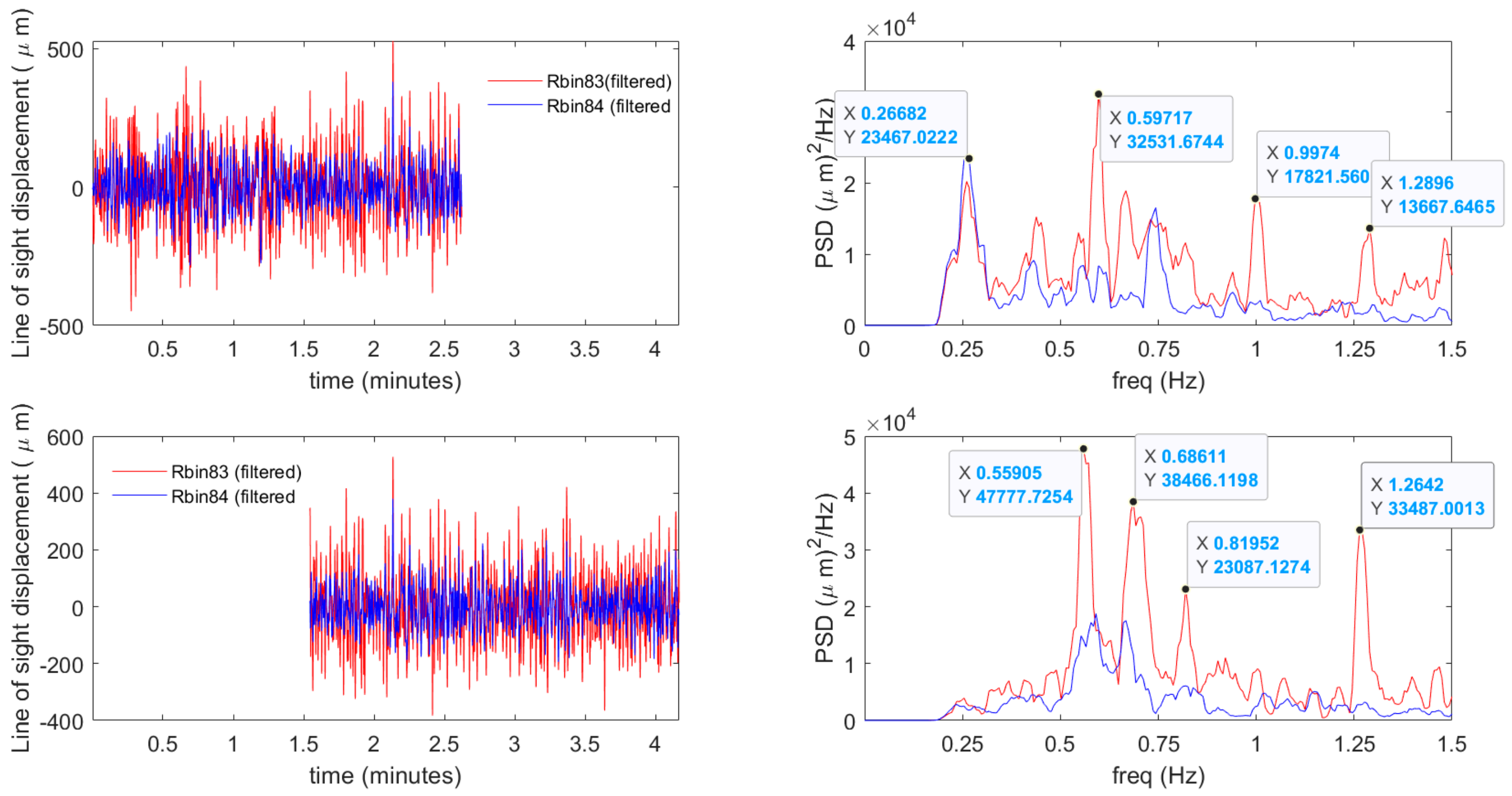
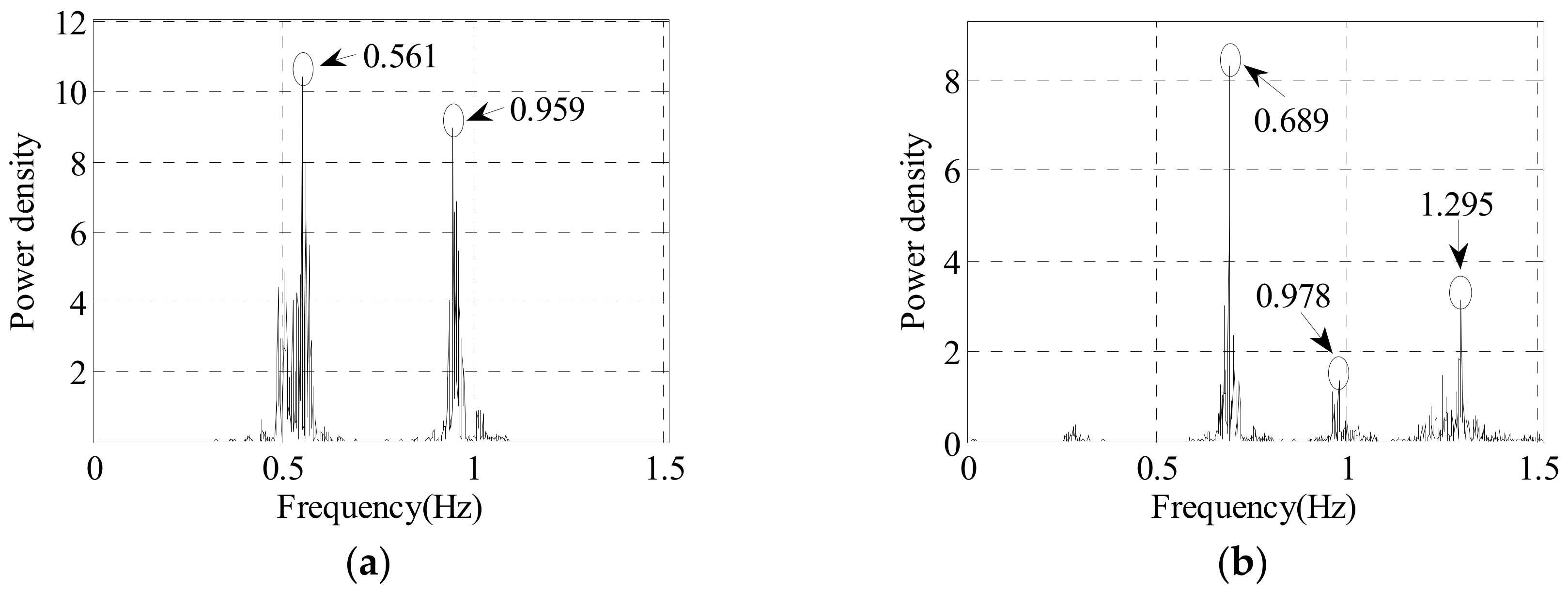
| 0.267 | ||
| 0.561 | 0.597/0.599 | |
| 0.689 | 0.686 | |
| 0.820 | ||
| 0.959 | ||
| 0.978 | 0.997 | |
| 1.295 | 1.264/1.290 | |
| Cases | Track No. | Direction | Carriages | Speed (km/h) |
|---|---|---|---|---|
| 1 | ② | S2N | 8 | 246.3 |
| 2 | ③ | N2S | 16 | 243.3 |
| 3 | ⑥/⑤ | S2N/N2S | Metro/16 | ~80/246.8 |
| 4 | ⑤/① | N2S/N2S | 8/Metro | 244.8/~80 |
| Cases | Track No. | Direction | Carriages | Speed (km/h) |
|---|---|---|---|---|
| C1 | ④ | S2N | 16 | 243.5 |
| C2 | ③ | N2S | 16 | 197.4 |
| C3 | ⑤ | N2S | 16 | 247.1 |
| C4 | ③ | N2S | 16 | 247.5 |
| C5 | ③&④ | N2S/S2N | 8/16 | 245.1/245.1 |
| C6 | ③ | N2S | 16 | 220.3 |
© 2020 by the authors. Licensee MDPI, Basel, Switzerland. This article is an open access article distributed under the terms and conditions of the Creative Commons Attribution (CC BY) license (http://creativecommons.org/licenses/by/4.0/).
Share and Cite
Huang, Q.; Wang, Y.; Luzi, G.; Crosetto, M.; Monserrat, O.; Jiang, J.; Zhao, H.; Ding, Y. Ground-Based Radar Interferometry for Monitoring the Dynamic Performance of a Multitrack Steel Truss High-Speed Railway Bridge. Remote Sens. 2020, 12, 2594. https://doi.org/10.3390/rs12162594
Huang Q, Wang Y, Luzi G, Crosetto M, Monserrat O, Jiang J, Zhao H, Ding Y. Ground-Based Radar Interferometry for Monitoring the Dynamic Performance of a Multitrack Steel Truss High-Speed Railway Bridge. Remote Sensing. 2020; 12(16):2594. https://doi.org/10.3390/rs12162594
Chicago/Turabian StyleHuang, Qihuan, Yian Wang, Guido Luzi, Michele Crosetto, Oriol Monserrat, Jianfeng Jiang, Hanwei Zhao, and Youliang Ding. 2020. "Ground-Based Radar Interferometry for Monitoring the Dynamic Performance of a Multitrack Steel Truss High-Speed Railway Bridge" Remote Sensing 12, no. 16: 2594. https://doi.org/10.3390/rs12162594
APA StyleHuang, Q., Wang, Y., Luzi, G., Crosetto, M., Monserrat, O., Jiang, J., Zhao, H., & Ding, Y. (2020). Ground-Based Radar Interferometry for Monitoring the Dynamic Performance of a Multitrack Steel Truss High-Speed Railway Bridge. Remote Sensing, 12(16), 2594. https://doi.org/10.3390/rs12162594