Article

Exploiting High-Resolution Remote Sensing Soil Moisture to Estimate Irrigation Water Amounts over a Mediterranean Region

1
Department of Civil and Environmental Engineering, University of Perugia, via G. Duranti 93, 06125 Perugia, Italy
2
National Research Council, Research Institute for Geo-Hydrological Protection, via Madonna Alta 126, 06128 Perugia, Italy
3
Observatori de l’Ebre (OE), Ramon Llull University—CSIC, 43520 Roquetes, Spain
4
isardSAT, Parc Tecnològic Barcelona Activa, Carrer de Marie Curie, 8, 08042 Barcelona, Spain
*
Author to whom correspondence should be addressed.
Remote Sens. 2020, 12(16), 2593; https://doi.org/10.3390/rs12162593
Submission received: 23 June 2020 / Revised: 15 July 2020 / Accepted: 8 August 2020 / Published: 12 August 2020

Abstract

:
Despite irrigation being one of the main sources of anthropogenic water consumption, detailed information about water amounts destined for this purpose are often lacking worldwide. In this study, a methodology which can be used to estimate irrigation amounts over a pilot area in Spain by exploiting remotely sensed soil moisture is proposed. Two high-resolution DISPATCH (DISaggregation based on Physical And Theoretical scale CHange) downscaled soil moisture products have been used: SMAP (Soil Moisture Active Passive) and SMOS (Soil Moisture and Ocean Salinity) at 1 km. The irrigation estimates have been obtained through the SM2RAIN algorithm, in which the evapotranspiration term has been improved to adequately reproduce the crop evapotranspiration over irrigated areas according to the FAO (Food and Agriculture Organization) model. The experiment exploiting the SMAP data at 1 km represents the main work analyzed in this study and covered the period from January 2016 to September 2017. The experiment with the SMOS data at 1 km, for which a longer time series is available, allowed the irrigation estimates to be extended back to 2011. For both of the experiments carried out, the proposed method performed well in reproducing the magnitudes of the irrigation amounts that actually occurred in four of the five pilot irrigation districts. The SMAP experiment, for which a more detailed analysis was performed, also provided satisfactory results in representing the spatial distribution and the timing of the irrigation events. In addition, the investigation into which term of the SM2RAIN algorithm plays the leading role in determining the amount of water entering into the soil highlights the importance of correct representation of the evapotranspiration process.

Graphical Abstract

1. Introduction

Human interventions into the natural circulation of water on the Earth’s surface can no longer be neglected in the global economy of the hydrological cycle. Abbot et al. [1] suggest that even the traditional representations of the cycle need to be adapted by involving anthropic water uses. Irrigation is a primary source of anthropogenic water consumption. It is estimated that over 70% of water withdrawals from lakes, rivers, and groundwater resources are destined for use in irrigation practices [2,3]. The continuous growth of the global population and the ever-rising living standards are expected to bring to an intensification of water depletion for improving agricultural production through irrigation practices, with higher impacts over areas already experiencing water stress conditions [4,5,6]. Climate changing scenarios coupled to the abovementioned phenomena are expected to further aggravate the problem. Hence, irrigation practices need to be adequately managed [7,8]. The knowledge of irrigation water amounts is essential not only for the important implications for food production and water scarcity, but for research purposes also. In fact, irrigation amounts often represent the missing information to adequately solve the water balance at several spatial scales [9,10].
Despite the primary role played by irrigation over human-altered basins, detailed quantitative knowledge of water amounts destined for this purpose is generally missing. Soil moisture has proven to be a key variable to retrieve information about occurred irrigation. From this perspective, several studies exploiting the SM2RAIN algorithm [11], which was originally developed to estimate rainfall from soil moisture observations and later adapted to estimate irrigation, provide promising results. Brocca et al. [12] showed the potential of the adapted version of the algorithm in reproducing irrigation amounts by exploiting coarse resolution satellite soil moisture. Jalilvand et al. [13] applied the SM2RAIN method with different settings for the evapotranspiration term to estimate irrigation water over the Miandoab plain, in Iran. Filippucci et al. [14] obtained good performances in estimating water applied for irrigation over a pilot field in Italy by exploiting in-situ soil moisture observations obtained through an advanced sensor based on Proximal Gamma-Ray spectroscopy as the SM2RAIN input. Alternative approaches exploiting soil moisture to estimate irrigation can be found in the literature. For instance, Zaussinger et al. [15] investigated the possibility to estimate the irrigation water use (IWU) over CONUS (CONtiguous United States) area through the differences between remotely sensed and modeled soil moisture. A similar approach was adopted by Zohaib and Choi [16], which showed the potential of microwave remote sensing in mapping irrigated areas and estimating IWU at a global scale by exploiting coarse resolution soil moisture observations from the ESA CCI (European Space Agency Climate Change Initiative) data set and soil moisture from ERA-5 (European ReAnalysis-5). However, soil moisture variation is not the only component of the hydrological cycle suitable to be exploited as a proxy of irrigation. In fact, irrigation practices also strongly affect the evapotranspiration process; hence, the evapotranspiration information can be useful to retrieve water amounts applied for irrigation. From this perspective, Romaguera et al. [17] exploited the differences between the remote sensing and modeled actual evapotranspiration to estimate monthly evapotranspiration rates due to irrigation over two study areas, the Horn of Africa and the province of Sichuan, in China. Peña-Arancibia et al. [18] proposed a methodology combining remote sensing data and hydrologic modeling to estimate the sources and the amounts of water consumed in the form of evapotranspiration from irrigated areas over two sub-basins of the Murray-Darling basin (Australia), which is known to be highly human-regulated. However, studies that quantitatively reproduce the irrigation amounts that actually occurred rather than showing potential applications in this sense or deriving information indirectly linked to irrigation are lacking.
The major novelty of this paper is to fill this gap. In order to do this, high-resolution (1 km) dDISPATCH (DISaggregation based on Physical And Theoretical scale CHange) downscaled versions of SMAP (Soil Moisture Active Passive) and SMOS (Soil Moisture and Ocean Salinity) soil moisture data sets have been used to force the SM2RAIN algorithm to estimate irrigation over an intensely irrigated area in the North East of Spain. The pilot area proved to be particularly suitable to investigate the detectability of the irrigation signal by remote sensing products and for irrigation mapping purposes [19,20,21,22,23]. The evapotranspiration term of the SM2RAIN equation has been improved by incorporating the guidelines about crop evapotranspiration furnished in the FAO (Food and Agriculture Organization) paper n. 56 [24]. Two experiments were carried out: one exploiting soil moisture from the SMAP at 1 km data set; and another one exploiting soil moisture from the SMOS at 1 km data set. The SMAP experiment covered the period from January 2016 to September 2017. The SMOS experiment, covering the period from January 2011 to September 2017, allowed a temporal extension back to the past of the estimated irrigation events.

2. Study Area

The pilot area is in the North East of the Iberian Peninsula. It is a 10,000 km2 tile (125 km by 80 km) located between two Spanish autonomous communities, Catalonia and Aragon. Within this area, a heavily irrigated land, on which this study is focused, is surrounded by a typical Mediterranean landscape characterized by sparse forests, shrubs, olive groves, and rainfed agricultural areas. The irrigated land is organized into four irrigation districts: the Urgell district, the Algerri Balaguer district, the Pinyana district, and the Catalan and Aragonese district (Canal de Aragón y Cataluña), whose Northern and Southern parts are fed by water coming from different reservoirs. Hence, in this study, the Catalan and Aragonese district has been divided into its Northern part (henceforth North Catalan Aragonese) and its Southern part (henceforth South Catalan Aragonese). Hence, a total of five districts were investigated. Figure 1 shows the location of the pilot site and the stations used to derive the benchmark irrigation volumes (except for the Pinyana district), the digital elevation model (DEM) of the irrigation districts, and the density of the equipment for irrigation. The DEM is derived from the EU-DEM v1.1 at 25 m resolution, delivered by the Copernicus Land Monitoring Service. The irrigation density, expressed according to three different levels, is derived from the geospatial information attached to the hydrological plan of the Ebro basin (available at the website http://www.chebro.es/contenido.visualizar.do?idContenido=42695&idMenu=4780), to which the study area belongs.
The districts differ from each other in terms of extension, dating, and irrigation techniques employed. In Urgell, flood irrigation is the most widespread technique; it is an old system in which irrigation generally occurs with a frequency of two weeks. The district has a total area equal to 887.62 km2 (8876,200 ha). The Algerri Balaguer district, with an area of 70.79 km2 (707,900 ha), can be considered the most pioneering one, as its irrigated area has been recently increased and new irrigation systems have been installed. In this district, irrigation can theoretically occur each day; drip irrigation is used for fruit trees and sprinklers for crops. In the Catalan and Aragonese district, several techniques coexist: flood irrigation (18% of the area), drip irrigation (28% of the area), and sprinkler irrigation (the most widespread technique, 54% of the area). The district has a total area equal to 1161.52 km2 (11615,200 ha); the Northern partition has an extension of 657.04 km2 (6570,400 ha), while the Southern one has an area of 504.48 km2 (5044,800 ha). No detailed information about the irrigation techniques adopted in the Pinyana district are available, but mixed techniques are supposed to be employed. The homonymous canal, which supplies water to the district, is the most ancient canal in the Catalonia autonomous community. The area of the district is equal to 149.74 km2 (1497,400 ha).

3. Materials and Methods

3.1. Remote Sensing Data

In this study two high-resolution soil moisture data sets were exploited: SMOS and SMAP at 1 km. Both products were obtained by downscaling the original resolution SMOS and SMAP data through the DISPATCH algorithm [25].
The SMOS mission was launched by the European Space Agency (ESA) at the end of 2009 [26] with the aim of collecting, over land, surface soil moisture estimates with a target accuracy of 0.04 m3/m3 [27]. The SMOS satellite is equipped with an Y-shaped passive 2D interferometric radiometer operating at L-band frequency (1.4 GHz) and provides surface soil moisture data with a spatial resolution ranging from 35 to 50 km, obtained through the Level-2 (L2) retrieval algorithm.
The SMAP mission was launched by the National Aeronautics and Spatial Administration (NASA) in January 2015 to collect hydrosphere state (surface soil moisture and freeze/thaw state) measurements at global scale [28]. The originally-designed SMAP equipment was an L-band radiometer (1.4 GHz) that, together with an L-band radar (1.26 GHz), was expected to provide soil moisture estimates at three different spatial resolutions (3 km, 9 km, and 36 km) by merging the advantages of both active and passive remote sensing. However, because of the radar failure in July 2015, only the 36 km and 9 km resolution products were delivered during the post-radar phase. Validation studies show that the retrieved surface soil moisture meets the mission target accuracy of 0.04 m3/m3 [29]. It is noteworthy that, after the identification of Sentinel-1A/Sentinel-1B SAR (Synthetic Aperture Radar) data as a suitable substitute of the SMAP radar derived data, a 3 km resolution combined product was delivered [30].
The DISPATCH method [31] allows the observed coarse resolution soil moisture to be disaggregated to finer resolutions by merging the microwave data with optical data. It is an evaporation-based downscaling algorithm that can be categorized as both theoretical and physically-based [32]. The downscaling is performed through the redistribution of the high-resolution soil moisture around the average value of the related coarser resolution product [33]. This process is allowed by the relationship existing between the soil evaporative efficiency (SEE), defined as the ratio of actual to potential evaporation, and the surface soil moisture [34]. In the DISPATCH method, the SEE is optical-derived, as it is estimated by exploiting the high-resolution (1 km) Normalized Difference Vegetation Index (NDVI) and land surface temperature (LST) data retrieved by MODIS (MODerate resolution Imaging Spectroradiometer) sensor aboard the Terra (EOS AM) and Aqua (EOS PM) satellites. The DISPATCH-derived products have been validated over several pilot areas with different climate conditions [25,35,36,37,38].
Two optical data sets have been used to estimate the crop coefficient evolution over the irrigated areas; they are the NDVI v2.2 and the Fraction of Vegetation Cover (FCover) v2 products, both at 1 km resolution, delivered by the Copernicus Global Land Service (CGLS). The products are obtained by processing the data retrieved by SPOT-VEGETATION (Satellite Pour l’Observation de la Terre - VEGETATION) and Project for On-Board Autonomy—Vegetation (PROBA-V) sensors. The VEGETATION instrument has been operational aboard the SPOT 4 and 5 Earth observation missions from April 1998 to May 2014. PROBA-V is a Belgian-led Earth observation mission developed by ESA and launched in May 2013 in order to ensure the continuity of the SPOT-VEGETATION mission observations; the VEGETATION imaging instrument has been redesigned adopting spectral channels similar to those of its former version. Further information on the PROBA-V mission can be found in Dierckx et al. [39], while the processing chain is described in Sterckx et al. [40].
Both products considered are provided at 10-day temporal frequency; the NDVI values vary between a minimum of -0.08 and a maximum of 0.92, while the FCover data set has a physical range of (0, 1). Detailed information about the products preparation, as well as validation reports, are accessible through the CGLS website (https://land.copernicus.eu/global/).

3.2. Meteorological Data

The meteorological variables used in this study were obtained through the SAFRAN (Système d’Analyse Fournissant des Renseignements Atmosphériques à la Neige) meteorological analysis system [41]. SAFRAN produces gridded data sets of rainfall rate, temperature, wind speed, and other meteorological variables; it combines a first guess coming from a numerical weather prediction model and ground-observed data through an optimal interpolation algorithm. The version of the data set used in this study is a SAFRAN originally implemented in Spain [42,43] with data until August 2014, which has been extended over the whole Iberian Peninsula (by involving Portugal) and until the end of August 2017; it is generated through minor changes to the code used for the SAFRAN implementation in France [44,45]. In this version, the ERA-Interim reanalysis, released by the European Centre for Medium-Range Weather Forecast (ECMWF), is used as a first guess for many variables, except for precipitation, whose first guess comes from observations recorded by the AEMET (Agencia Estatal de METeorología) meteorological station network, which is also the source of the ground observations for the interpolation.
The meteorological data are provided gridded on a 5 km resolution grid and at an hourly time step; hence, they have been aggregated ata daily time scale and resampled to the finer resolution (1 km) adopted in this study. The variables exploited were: the rainfall rate, the relative humidity, the temperature, and the wind speed; the first one has been used as reference precipitation in the SM2RAIN elaborations, while the others, together with the solar radiation data from the ERA-5 reanalysis [46], resampled to the same grid used for SAFRAN, were used to calculate the potential evapotranspiration according to the FAO Penman-Monteith method.

3.3. Benchmark Irrigation Volumes

The ground truth values of irrigation water considered in this study are deduced by several sources. For the experiment exploiting soil moisture from the SMAP at 1 km data set, covering the period from January 2016 to September 2017, the benchmark irrigation amounts are mainly deduced by the volumes of water flowing through the irrigation canals network and feeding the districts. These data, available in real time and as historical collections, are delivered by the Automatic Hydrologic Information System of the Ebro river basin (SAIH Ebro) at the website: http://www.saihebro.com/saihebro/index.php?url=/datos/canales. This kind of benchmark irrigation data has been used for all the pilot districts, except for the Pinyana district, which is not included in the SAIH system. The stations exploited for this purpose are shown in Figure 1 and reported in Table 1. The data for water supplying the Urgell district are missing during the period going from July 2016 to February 2017; hence, for the sub-period from January to September 2017, the data from February to September 2017 have been used, by assuming that the missing amount referred to January 2017 is negligible. For the 2016, as the missing data covers a considerable part of the high-intensity irrigation season, a secondary benchmark value taken from the Hydrological Plan of the Spanish Part of the Ebro River Basin has been considered. This data is a yearly cumulated estimation based on historical data referring to a twelve-years period (from 2000 to 2012). For the Pinyana district, monthly volumes of irrigation water have been furnished by the canal’s technical office.
The benchmark irrigation volumes were converted to the equivalent thickness of irrigation water (in mm) to be compared with satellite-derived irrigation estimates by dividing them by the area of each district. It is noteworthy that, for the Urgell district, a very small part with low irrigation density has not been considered.
Only the portion of water that actually reaches the soil can be measured through remote sensing. For this reason, the gross benchmark irrigation amounts have been reduced by considering the losses due to irrigation efficiency. The entities of the losses have been set by considering the dating of the irrigation systems, the irrigation techniques, and previous studies investigating this topic over the pilot area. Canela et al. [47] evaluated the efficiency of the flood irrigation system in Urgell, defined as the capability of the applied water to reach the root zone. The authors found lower efficiencies in the upper part of the district (mean efficiency of 66%) with respect to the lower part (mean efficiency of 90%). A mean irrigation efficiency of 77% over the Urgell was found by Cots et al. [48]. Matè et al. [49] investigated the efficiency of the flood irrigation system over selected crops within the Catalan and Aragonese district. The obtained efficiency varied between 62% for the sunflower and 89% for fruit trees. In general, it is well known that losses due to a flood irrigation system are expected to be higher with respect to those due to sprinkler systems. Drip irrigation systems should ensure the maximum efficiencies. On the basis of the abovementioned considerations, losses equal to the 30% of the delivered amounts of water have been adopted for the Urgell district, where flood irrigation is the most widespread technique. For the Catalan and Aragonese district, considering that mixed techniques are employed, the losses are assumed to be equal to 15% of the total. Losses equal to 10% of the water pumped to the Algerri Balaguer district have been assumed, as this system is the most recent one. Conversely, for the Pinyana district, which is the most ancient system among those evaluated, losses equal to the 30% of the water supplying the district have been assumed.
For the SMOS experiment, the same sources of benchmark irrigation have been used for the Catalan and Aragonese and the Algerri Balaguer districts. For the Urgell district, the prevision based on historical data, already used for 2016, has been used as a fixed value for the previous years also. It has not been possible to obtain benchmark irrigation volumes for the Pinyana district during the period 2011–2015. The net irrigation benchmark values, expressed as irrigation water thickness and taking into account of losses due to the irrigation efficiency, have been obtained through the same procedure previously described for the SMAP experiment. Table 1 summarizes the areas considered for the conversion of irrigation volumes to irrigation thicknesses, the sources of the benchmark data, and the assumed losses.

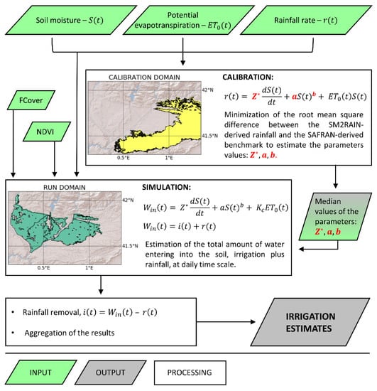
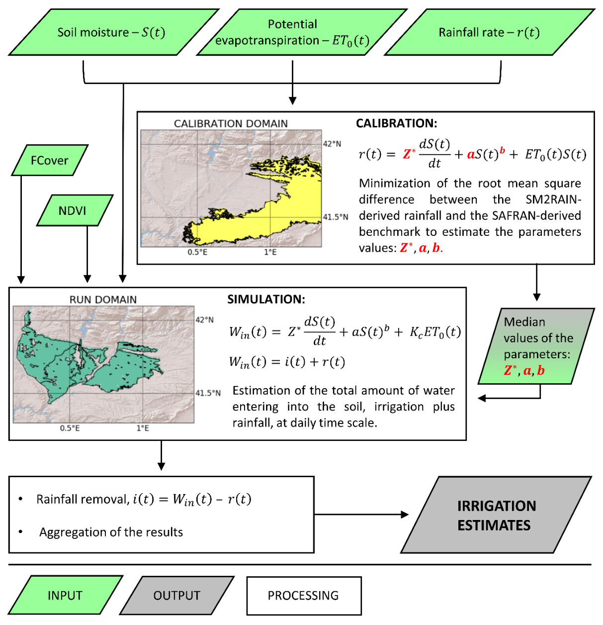
3.4. The SM2RAIN Algorithm

An adapted version of the SM2RAIN algorithm has been used to estimate the irrigation water amounts. The algorithm was originally developed to retrieve rainfall through an inversion of the water balance with soil moisture variations as input [11,50,51], then it has been adapted for quantifying irrigation [12]. Indeed, over agricultural areas, the SM2RAIN output is actually an estimate of the total amount of water entering into the soil, irrigation plus rainfall.
The soil water balance equation, in its general form, can be expressed by:
n Z d S ( t ) d t = i ( t ) + r ( t ) g ( t ) s r ( t ) e ( t ) ,
where n [−] is the soil porosity, Z [mm] is the soil layer depth, S ( t ) [−] is the relative soil moisture, t [days] is the time, i ( t ) [mm/day] is the irrigation rate, r ( t ) [mm/day] is the rainfall rate, g ( t ) [mm/day] is the drainage (the sum of deep percolation and subsurface runoff) rate, s r ( t ) [mm/day] is the surface runoff and e ( t ) [mm/day] is the actual evapotranspiration. The Equation (1) can be also written in its equivalent form:
n Z d S ( t ) d t = W i n ( t ) g ( t ) s r ( t ) e ( t ) ,
where W i n ( t ) = i ( t ) + r ( t ) [mm/day] is the total amount of water entering into the soil. By adopting the assumptions described in the following sections, Equation (2) allows the total amount of water entering into the soil, W i n ( t ) , to be determined; hence, by removing the rainfall signal, the irrigation rate can be estimated.
In the method presented in this study, the SM2RAIN algorithm has been employed in two different configurations, one for the model’s parameters calibration and another one for the irrigation estimates.
Two SM2RAIN experiments were carried out. The first one represents the core simulation of this study, which covers the period ranging from January 2016 to September 2017 and exploits SMAP at 1 km soil moisture data. The second one is an extension back to 2011 of the former analysis and exploits remote sensing soil moisture from the SMOS at 1 km data set. Both products proved to be skillful in detecting the irrigation signal over the pilot area [23].

3.4.1. Calibration

The calibration phase was performed over the dryland surrounding the irrigated land on the East side (see Figure 2). It is an area mainly constituted of rainfed cropland mixed with olive groves and shrubs, and sparse forests are also present. Over this domain, there is no irrigation; hence, the i ( t ) term is equal to zero and the total amount of water entering into the soil is represented by rainfall only, W i n ( t ) = r ( t ) . Equation (2) is rewritten in the following form:
Z * d S ( t ) d t = r ( t ) g ( t ) s r ( t ) e ( t ) ,
with Z * = n Z [mm] representing the water capacity of the soil layer. The drainage rate and the soil moisture are assumed to be related through a power law equation: g ( t ) = a S ( t ) b , with a and b drainage parameters. The rate of the surface runoff is assumed to be negligible. The actual evapotranspiration is assumed to be equal to the potential one, E T 0 ( t ) [mm/day], limited by the available water content: e ( t ) = E T 0 ( t ) S ( t ) . The potential evapotranspiration has been calculated according to the FAO Penman-Monteith method [24]:
E T 0 ( t ) = 0.408 Δ ( R n G ) + γ 900 T + 273 u 2 ( e s e a ) Δ + γ ( 1 + 0.34 u 2 ) ,
where Δ [kPa/°C] is the slope of the vapor pressure curve, R n [MJ/m2day] is the net radiation at the crop surface, G [MJ/m2day] is the soil heat flux density, T [°C] is the mean daily air temperature at 2 m height, u 2 [m/s] is the wind speed at 2 m height, e s [kPa] is the saturation vapor pressure, e a [kPa] is the actual vapor pressure and γ [kPa/°C] is the psychrometric constant. Equation (4) was obtained from the original Penman-Monteith equation [52,53] and it refers to a terrestrial surface characterized by a standard grass crop of 12 cm height, a fixed surface resistance of 70 s/m, and a fixed albedo equal to 0.23. All the components of Equation (4) have been derived from four fundamental meteorological variables: the air relative humidity, the wind speed, the air temperature, and the solar radiation.
Applying the above mentioned assumptions, Equation (3) is rewritten as:
r ( t ) = Z * d S ( t ) d t + a S ( t ) b + E T 0 ( t ) S ( t ) ,
and the reference SAFRAN rainfall rate can be used to calibrate the three model’s parameters: Z * , a , b . The calibration procedure is performed through an objective function aimed to minimize the root mean square difference between the SM2RAIN-derived rainfall, calculated using Equation (5), and the SAFRAN-derived benchmark rainfall. For both experiments performed, the calibration was carried out by adopting a 5-day temporal aggregation, which proved to be the one maximizing the performances in terms of rainfall estimation. The process provides the distributions of Z * , a , and b over the calibration domain; hence, the median values are used as fixed parameters for the irrigation estimate.

3.4.2. Irrigation Estimates

The simulation step, aimed at estimating the irrigation amounts, was carried out for the selected districts. Over the irrigated crops the total water entering into the soil is the sum of the irrigation and rainfall rates, W i n ( t ) = i ( t ) + r ( t ) . In this step, the assumptions adopted for the surface runoff and the drainage rate for the calibration process were still valid. The evapotranspiration, e ( t ) , was modeled by integrating the dual crop approach proposed in the FAO paper n. 56 [24]. According to this model, the crop evapotranspiration was obtained from the reference potential one multiplied by the crop coefficient, K c [−], which describes the crop development:
e ( t ) = K c E T 0 ( t ) ,
in the dual crop coefficient approach, the contributions of the evaporation from bare soil and the crop transpiration are evaluated separately by splitting the crop coefficient as the sum of two terms:
K c = K c b + K e ,
where K c b [−] is the basal crop coefficient, describing the plant transpiration component, and K e [−] is the soil water evaporation coefficient and represents the evaporation from the soil surface. In order to take into account of stress conditions due to limited available water for the crops, Equation (7) can be generalized in the form:
K c = K s K c b + K e ,
with K s [−] representing the water stress coefficient. The FAO guidelines provide equations to calculate K s , K c b , and K e . The multitude of the required variables and the detailed knowledge of each single crop at plot scale make the rigorous calculation of the parameters difficult over an extended and crop-composite area as that of interest of this study. Hence, for each coefficient, empirical parametrizations exploiting remotely sensed data have been developed. Optical products have proven to be useful tools for assessing crop evolution [54]. Many authors have highlighted the linear relation existing between K c b and the NDVI [55,56,57,58,59], to cite a few. In the proposed approach, K c b is obtained, for each irrigated pixel, by scaling the NDVI between its maximum and a minimum value assumed equal to 0.2, thus obtaining K c b values ranging between 0.2 and 1. Water limitation stress is taken into account by linking K s with soil moisture. Defined p as a soil moisture threshold below which stress occurs, the coefficient is calculated as:
{ K s = S ( t ) p ,     S ( t ) < p     K s = 1 ,     S ( t ) p ,
When the relative soil moisture is higher than the stress threshold, there is no stress ( K s = 1 ), while when water content drops below the threshold value, K s decreases linearly. For both the experiments carried out, p has been set equal to 0.45, meaning that stress starts when the relative surface soil moisture drops below the 45%. This threshold value was found to be the most suitable one to reproduce the long-term irrigation magnitudes. It is noteworthy that, for both experiments, the stress condition is not frequently reached; furthermore, the beginning of the stress is established through a surface soil moisture threshold, but in the root zone water can still be available. According to the FAO guidelines, K e has an upper limit linked with the fraction of soil surface wetted and exposed, where evaporation occurs, and with a maximum K c value which ensures the non-exceedance of the available energy. In this study, rather than an energy-based limitation, a water-based limitation is assumed. The evaporation from the soil surface is formulated as follows:
K e = ( 1 f c ) S ( t ) ,
where f c is the fraction of vegetation cover, for which the FCover data set is used. This assumption is equivalent to state that, over the portion of bare soil of an irrigated pixel, the evaporation is limited by the available water content. Equation (10) is consistent with the assumption made for the actual evapotranspiration over the calibration domain, where the process has been modeled through a coarser approach with respect to the modeling adopted over the irrigated areas since the transpiration part is not predominant.
Over the irrigation districts, applying the above mentioned assumptions, Equation (2) can be reformulated as follows:
W i n ( t ) = Z * d S ( t ) d t + a S ( t ) b + K c E T 0 ( t ) ,
where the SM2RAIN parameters are fixed to their median values resulting from the calibration step. By solving Equation (11) it is possible to estimate the total amount of water entering into the soil at daily time scale. Hence, the irrigation rate can be estimated by removing the rainfall rate from this amount of water, i ( t ) = W i n ( t ) r ( t ) . It is noteworthy that, when the i ( t ) term was negative, it was assumed equal to zero. The flow chart in Figure 2 provides an overview of the whole procedure employed in this study to estimate the irrigation amounts.

3.4.3. Assessment of the Parameters Uncertainty

For the experiment exploiting SMAP at 1 km soil moisture, an analysis of the uncertainty due to the model parameters was carried out. The sensitivity of the results obtained to the three SM2RAIN parameters involved in the calibration step ( Z * , a , and b ) was evaluated separately from the uncertainty linked to the soil moisture threshold, p , which determines the beginning of stress conditions. As specified in the previous section, the irrigation estimates step was carried out by fixing the parameters Z * , a , and b equal to the median values of their distributions over the calibration domain. In order to assess the model sensitivity to Z * , a , and b , a set of alternative simulations adopting random combinations of the parameters were performed; this process allowed us to build a confidence interval around the main simulation presented in this study. The 25th, 50th, and 75th percentiles of the distributions of the three SM2RAIN parameters have been chosen and combined together according to all possible combinations. A total of 27 simulations were performed; note that they were 26 plus the main one performed by adopting the median values of the parameters distribution, which corresponds to considering the 50th percentile of each parameter. The evaluation of the sensitivity to the stress threshold has been carried out by performing the main simulation (in which Z * , a , and b are fixed to their median values resulting from the calibration step) and varying p between 0.3 and 0.6 with steps of 0.01. The confidence interval around the main simulation has been built through the 30 additional simulations resulting from this procedure.

3.5. Remote Sensing and Meteorological Data Preparation

All the remotely sensed and meteorological data sets used have been resampled to the same 1 km grid; this procedure allowed us to perform the analyses described in this study with spatially coherent data. The coarser resolution data sets were first resampled to a 1 km regular grid through the nearest neighbor method, then a second resampling through linear interpolation to the points of the 1 km grid adopted in this study was performed. The data sets at 1 km resolution were only resampled to the adopted grid through linear interpolation.

4. Results

4.1. Experiment with SMAP at 1 km Soil Moisture

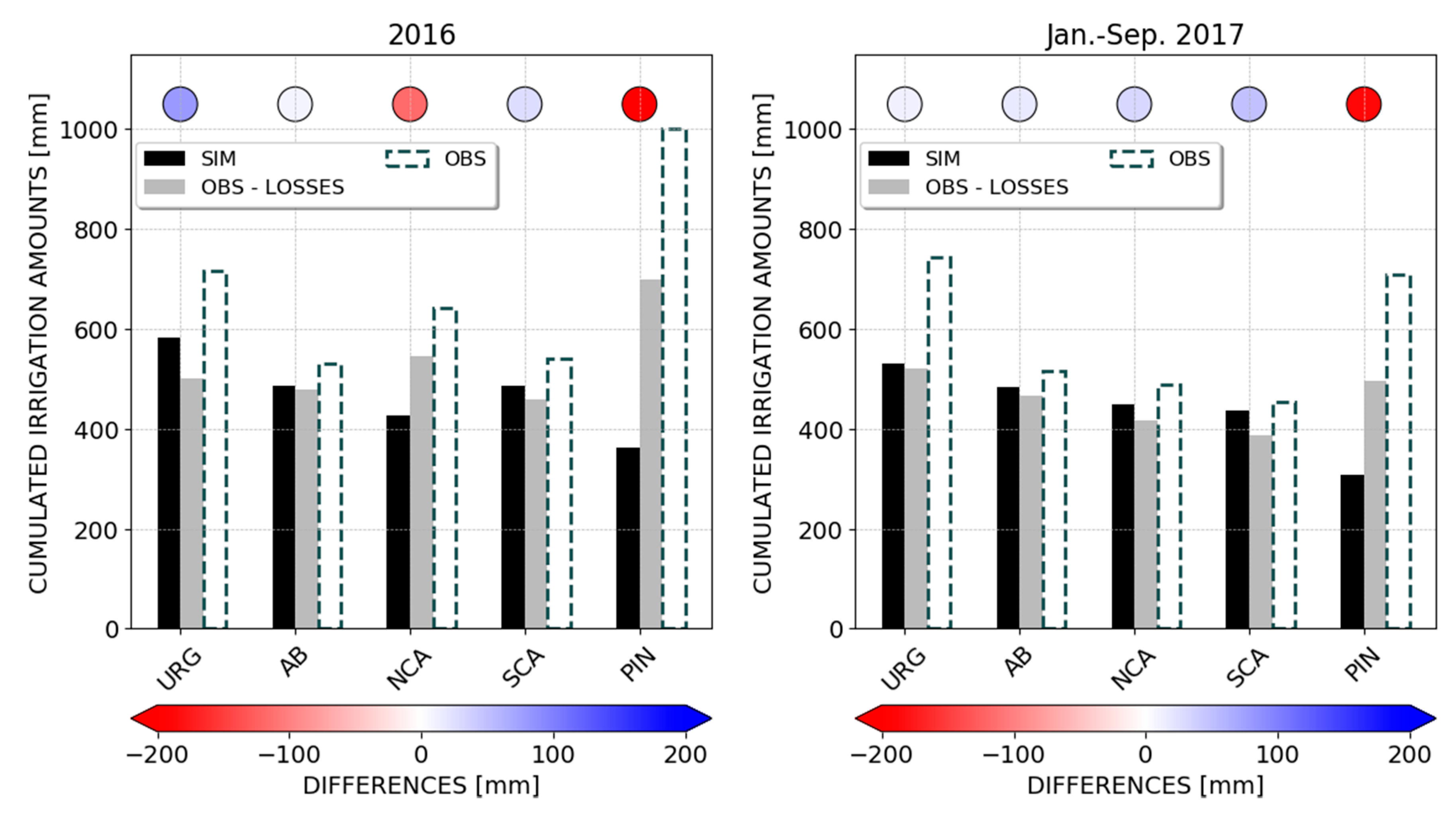
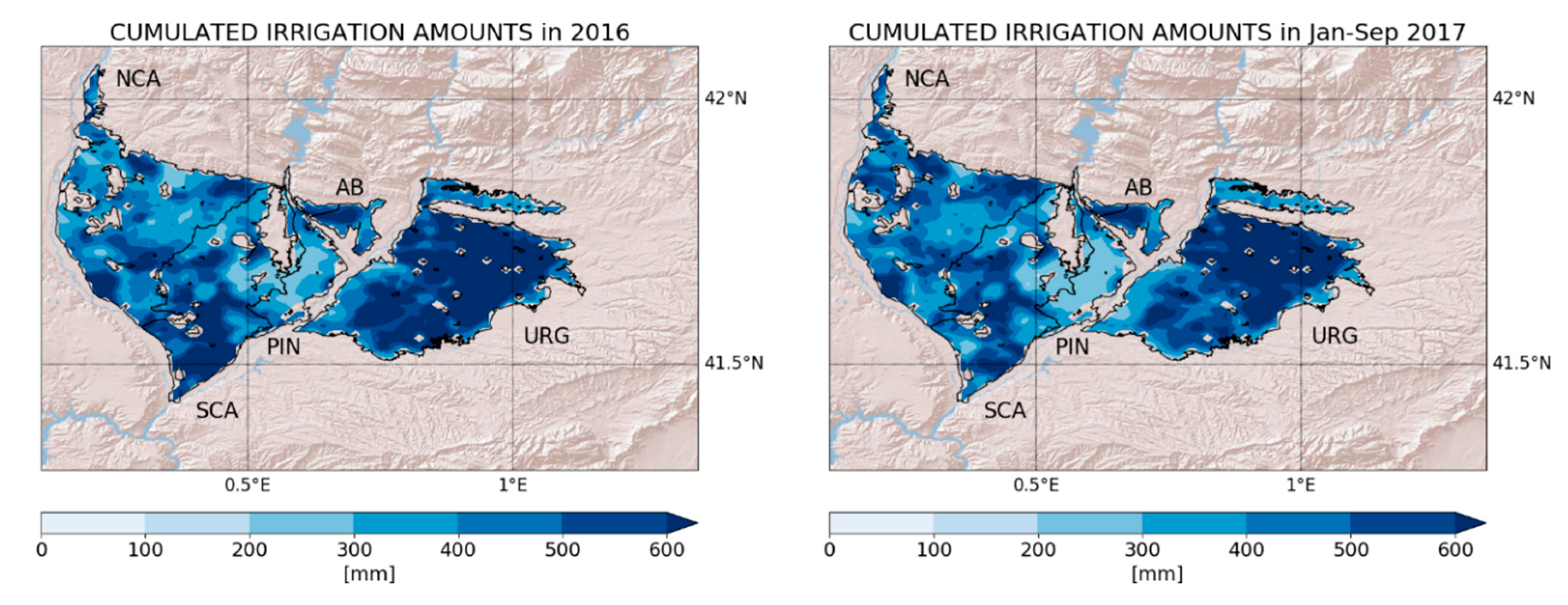
4.1.1. Irrigation Estimates

In the experiment exploiting SMAP at 1 km soil moisture, the amounts of irrigation water feeding the pilot districts during a 20-month period, from the beginning of 2016 to September 2017, were estimated and compared with benchmark data. The calibration step, performed over the dryland surrounding the irrigated areas during the same temporal span of the irrigation estimate experiment, provided the following values for Z * , a , and b : Z * = 32.930 mm, a = 0.882 mm, and b = 7.704; these values were fixed for each pixel of the irrigated domain during the irrigation estimates phase. Figure 3 shows the time series of the estimated irrigation, spatially averaged for each district, together with reference amounts and the spatial mean of rainfall from SAFRAN; the time series referring to Urgell, Algerri Balaguer, and North and South Catalan and Aragonese districts were aggregated at 5 days; for the Pinyana district, the results were aggregated monthly (in accordance to the temporal aggregation of the benchmark data) and represented through bars. An evaluation of the performance of the proposed method in estimating irrigation is given though the RMSE and the Pearson correlation coefficient ( r ), calculated by considering aggregated values of the estimated amounts against the benchmark ones with losses due to the irrigation efficiency taken into account. For the Urgell district, good accordance between estimated and benchmark irrigation can be observed, even if the analysis is limited by the missing data in the ground truth irrigation volumes. RMSE equal to 4.37 mm/5-days and r equal to 0.73 are obtained. A slightly higher RMSE, equal to 6.11 mm/5-days, was obtained over the Algerri Balaguer district, for which r remains satisfactory (0.76). Over this area, underestimates during the peaks of the irrigation season (from July to September) and false irrigation during the winter season were detected. For the North Catalan and Aragonese area, the lowest r value is obtained (0.58), while a good RMSE value, equal to 4.20 mm/5-days, can be observed. The South Catalan and Aragonese domain is where the best overall performances were obtained, with RMSE equal to 3.04 mm/5-days and r equal to 0.82. For the Pinyana district, even if the agreement between monthly increases and decreases of the estimated and observed irrigation amounts was good ( r = 0.81), the proposed method strongly underestimated reference irrigation data (RMSE = 36.85 mm/month). It is noteworthy that, although the RMSE values obtained for Pinyana and Algerri Balaguer are comparable, they have a different origin; over the Algerri Balaguer district the error was mainly determined by slight underestimates during the highest irrigation intensity periods together with false irrigation in winter, while over the Pinyana district the error was mainly determined by systematic underestimates.
A comparison between the long-term magnitudes of estimated and benchmark irrigation amounts is provided in Figure 4. For each district, the estimated irrigation amounts (black bars) are represented together with the benchmark amounts reduced by the losses due to the irrigation efficiency (light grey bars), representing the actual reference, and with the gross benchmark amounts (bars with dashed edges). The differences between the estimated and benchmark long-term magnitudes are expressed by the color of the circles above the bars; underestimates are represented in red and overestimates in blue. Except for the Pinyana district, for which strong underestimates (–337.57 mm in 2016 and −186.75 mm in January–September 2017) were obtained, the long-term magnitudes of real irrigation were well reproduced by the proposed method. For the Urgell district, the Algerri Balaguer district, and the South Catalan and Aragonese area, good agreement between simulated and observed cumulated irrigation amounts was obtained. A slight overestimate (+80 mm) over the Urgell in 2016 can be observed. Over the North Catalan and Aragonese area, the proposed method underestimated the real irrigation in 2016 (−116.97 mm), while good agreement can be observed during the period January–September 2017.
The spatial distribution of irrigation estimates obtained through the SM2RAIN algorithm and cumulated for the 2016 and for the period January–September 2017 is shown in Figure 5. Even with slightly different magnitudes, both maps show similar patterns. The Urgell district, where flood irrigation mainly occurs, shows evenly distributed high cumulated irrigation amounts. In the Algerri Balaguer district, a pattern of intense irrigation can be observed in its West side, corresponding to the original extension of the district. Over the Northern and Southern partitions of the Catalan and Aragonese district, recursive high irrigation amounts can be detected in certain areas. The estimated irrigation was evenly scarce over the whole Pinyana district. It is noteworthy that the distributions of the SM2RAIN-derived irrigation estimates are consistent with maps of actually irrigated areas over the same pilot area proposed by the authors in Dari et al. [23].
Besides the irrigation estimates, it is interesting to investigate which process among those modeled into SM2RAIN contributes the most in determining the model output. For each irrigation district, the spatially averaged contributions to the total amount of water entering into the soil (rainfall plus irrigation) of each term of the SM2RAIN equation are shown in Figure 6. The red shaded area is the drainage contribution, the blue shaded area is the soil moisture variation contribution, and the green shaded area represents the actual evapotranspiration term; the total amount of water entering into the soil is represented by the black line. The districts-averaged rainfall rates (blue bars) and estimated irrigation rates (magenta bars) are also shown. The pie charts represent, for each district, the percentages of the various contributions to the total. It is noteworthy that, while the e ( t ) and g ( t ) terms are fluxes and are always positive contributions, the n Z d S ( t ) / d t term represents a change in a stock, which can be both positive or negative. In fact, in the absence of rainfall or irrigation events, the soil moisture decreases, and thus a negative term for this component is necessary to solve the balance and equilibrate the positive drainage and evapotranspiration terms, which represent a consumption of the available water content in the control volume of soil. Furthermore, the soil moisture plays an indirect role that consists of modulating the potential evapotranspiration over bare soil. For all these reasons, the percentages of each term shown in the pie charts have been calculated only when the n Z d S ( t ) / d t term is positive, i.e., after rainfall or irrigation events; hence, only the direct contribution of soil moisture variation was considered. For all of the districts, the drainage term was negligible; it ranged between 0.2% and 0.4% of the total. This result is consistent with recent studies exploiting coarser resolution soil moisture products [13]. The direct soil moisture variation contribution varies between 38.5% and 45.7% of the total; for all the districts, the actual evapotranspiration term is the predominant one, with percentages ranging between 54.0% and 61.1% of the total.

4.1.2. Estimate of the Model Parameters Uncertainty

The main results of the assessment of the uncertainty due to the SM2RAIN parameters Z * , a , and b are shown in Figure 7. For each district, the 10-day aggregated spatial mean of the irrigation amounts estimated through the main simulation described in the preceding section by adopting fixed parameters equal to the median values of their distributions is represented through the black line. The 26 additional simulations obtained through the random combination of the 25th, 50th, and 75th percentiles of each parameter distribution are represented in light grey; the additional simulations allow to build a confidence interval useful to assess how much the proposed irrigation estimates are sensitive to the SM2RAIN model parameters Z * , a , and b . The amplitude of the confidence interval is expressed by the upper horizontal bar. Over each selected district, during the highest irrigation intensity periods, i.e., from May to September 2016 and 2017, the amplitude of the confidence interval was very small (less than 2–3 mm/10-days). Outside these time intervals, an increase up to a maximum reached at the end of 2016 can be observed. The maximum detectable amplitude varied between 7.1 mm/10-days (for the Algerri Balaguer district) and 9.7 mm/10-days (for the Pinyana district).
An additional parameter is involved in the irrigation estimate phase, p . It represents the soil moisture threshold determining the beginning of stress conditions. The results of the assessment of the sensitivity to this parameter are provided in Figure 8. The black line represents the 10-day aggregated spatial mean of estimated irrigation for each pilot district through the main simulation; the 30 additional simulations, obtained by varying the p value between 0.3 and 0.6 with steps of 0.01, are represented in light grey. The amplitude of the resulting confidence interval is expressed by the upper horizontal bar. Conversely, from the results on the model’s sensitivity to Z * , a , and b , the uncertainties linked to p were mainly observed during the highest irrigation intensity periods. This is an expected result, as the p parameter affects the crop evapotranspiration. The maximum amplitudes of the confidence interval were detected in the summer 2017 and range between 11.1 mm/10-days (for the Pinyana district) and 14.7 mm/10-days (for the South Catalan and Aragonese district).

4.2. Experiment with SMOS at 1 km Soil Moisture

An alternative experiment exploiting remotely sensed soil moisture from the SMOS at 1 km data set, performed by adopting the same flow chart described for the experiment with the SMAP at 1 km data set, has been carried out. The longer time series available for this data set allowed the irrigation estimates to be extended back to 2011. Both DISPATCH downscaled products proved to be able to detect the irrigation signal over the pilot area [23]; hence, the SMOS experiment has a dual objective, i.e., to compare the performances of the two considered products during the period covered by both the experiments (from January 2016 to September 2017) and to estimate yearly cumulated irrigation amounts before 2016. The calibration step, performed like the SMAP-based one by minimizing the root mean square difference between the SM2RAIN-derived rainfall and the rainfall rate from SAFRAN over the selected non-irrigated area, provides the following results: Z * = 22.896 mm, a = 13.770 mm and b = 3.864.
The results of the irrigation estimate are shown in Figure 9, where, for each district, the cumulated irrigation amounts estimated with SMOS at 1 km data set (orange bars) and SMAP at 1 km data set (black bars) are represented together with the benchmark values reduced by considering the losses due to irrigation efficiency (light grey bars) and with the gross benchmark values (bars with dashed edges). The colors of the circles above the bars express the magnitude of underestimates (red) or overestimates (blue) deductible from the differences between estimated irrigation amounts referred to the SMOS experiment and the actual benchmark.
For the Catalan and Araganose district (both its Northern and Southern partitions) and the Pinyana district, the experiments provided comparable long-term magnitudes of estimated irrigation amounts. It is noteworthy that, over North and South Catalan and Aragonese districts, the SMOS experiment even slightly enhanced the performances obtained with the SMAP experiment. Over the Urgell district and the Algerri Balaguer district, the SMOS experiment produced lower irrigation estimates with respect to the SMAP experiment. This issue can be explained by sources of radio-frequency interference (RFI) detected in these districts since mid-2016 and already pointed out in Dari et al. [23]. In the case of RFI problems, the worst performances of SMOS with respect to SMAP, designed with a RFI filter onboard, are a known issue [60]. Regarding the performances in reproducing the actually-occurring irrigation obtained through the SMOS experiment, the magnitudes of estimated irrigation amounts are generally consistent with the benchmark. It is noteworthy that it has not been possible to collect benchmark data referred to the period 2011–2015 for the Pinyana district. However, the similitudes of the magnitudes obtained to the SMAP experiment suggest that real irrigation in this district is confirmed to not be well reproduced by the proposed method. Over the Urgell and the Algerri Balaguer districts, the SMOS soil moisture-derived irrigation estimates adequately reproduced the observed irrigation amounts until 2016, when the abovementioned RFI problems began. Significant underestimates (up to −185.93 mm) were obtained over the Northern partition of the Catalan and Aragonese district during the period 2013–2015. This issue was not detected for the Southern partition of the district, over which the irrigation that actually occurred was always well reproduced by the experiment exploiting the SMOS at 1 km data set.

5. Discussion

In this study, a method able to reproduce the irrigation amounts that actually occurred over a semi-arid region through high-resolution soil moisture products is proposed. The pilot area, rich in terms of irrigation data, allowed the robustness of the method to be assessed.
The proposed analysis closes the gap between the potential of coarse resolution remote sensing soil moisture data to detect irrigation and the need of high-resolution products to solve the small-scale irrigation signal, thus adequately estimating irrigation, already pointed out in previous studies [12,15].
The method performs well in estimating the irrigation that actually occurred over four of the five pilot districts, despite the slightly different results. Where the method performs well, not only were the long-terms magnitudes adequately reproduced, but the irrigation timing was too. In fact, the RMSE remained low, varying between 3.04 mm/5-days for the Southern part of the Catalan and Aragonese district and 6.11 mm/5-days for the Algerri Balaguer district, while the correlation ranged between 0.58 for the Northern partition of the Catalan and Aragonese district and 0.82 of its Southern partition. It is interesting to note that non-negligible irrigation events that occurred in the winter 2016 over the North Catalan and Aragonese area are reproduced by the proposed method. During the same period, small irrigation events not reflected in the benchmark data can be detected over the Algerri Balaguer; these events can be false irrigation alarms produced by SM2RAIN or real irrigation water supplied with a certain delay with respect to the time when it has been pumped from the river. In fact, the district is equipped with three reservoirs that can furnish water to the crops later than when the same water is pumped to the district. This issue can also explain the underestimates during the summer; the water pumped to the district was used as the reference real irrigation, but it may happen that a part of it is immediately sent to the crops and another part is stored in reservoirs and dispensed later. In addition, delays between the pumping of water to the district and the water supply to the crops may negatively affect the RMSE and r values obtained for the Algerri Balaguer district.
The unsatisfactory performances in estimating irrigation events over the Pinyana district can be attributed to several complementary causes, such as a “contamination” by an adjacent non-irrigated area, as well as uncertainties associated to the benchmark irrigation volumes. In fact, the Pinyana irrigation system is the most ancient one among those examined in this study and it is possible that the actual losses due to the distribution efficiency are higher than supposed. This study also highlights the importance of a correct representation of the evapotranspiration process when the SM2RAIN method is applied over a semi-arid region, as already pointed out by Jalilvand et al. [13]. The evapotranspiration term plays the leading role in determining the total amount of water entering the soil according to the SM2RAIN equation, higher than the direct contribution of soil moisture. However, soil moisture also plays an indirect role in evapotranspiration estimation, whose effects are difficult to quantitatively estimated. Indeed, in the proposed water-limited approach, the soil moisture modulates the potential evapotranspiration over the portions of irrigated pixels not covered by vegetation and regulates the stress conditions due to water scarcity.
The assessment of the uncertainties linked to the SM2RAIN parameters show that irrigation estimates are scarcely affected by variations of the model’s parameters Z * , a , and b . In fact, when irrigation mainly occurs, the amplitude of the confidence interval around the main simulation obtained in the SMAP experiment reaches its minimum values. Conversely, larger amplitudes were detected at the end of 2016. The analysis of the uncertainties linked to the p parameter revealed meaningful sensitivity of the SMAP-derived irrigation estimates when irrigation mainly occurs, as this parameter affects the crop evapotranspiration process. In the FAO model, stress conditions are considered by determining the fraction of the total available water for crops, namely the water in the root zone, which is derived by tables with reference values for each crop. A fraction equal to 0.5 is adopted for many crops. In the proposed parametrization, the stress condition is taken into account on the basis of a surface soil moisture threshold. Hence, the entire water profile into the soil is not considered. In addition, the threshold is static in space and time. The building of a dynamic representation both in space and time for p , in which the parameter varies for different crops and in time, is among the future perspectives of this study.

6. Conclusions

This study highlights the capability to estimate the amounts of water actually applied for irrigation practices by forcing the SM2RAIN algorithm with DISPATCH downscaled high-resolution soil moisture. In order to do this, detailed modeling of the crop evapotranspiration according to the FAO method was included in the algorithm. On the basis of the results discussed above, the following conclusions can be drawn:
  • the proposed method is able to quantitatively estimate the irrigation that actually occurred over the study area, at least for four of the five irrigation districts considered;
  • the method proved to be suitable not only to estimate the long-term irrigation magnitudes, but also to represent the spatial distribution and the timing of irrigation events;
  • over semi-arid regions, the evapotranspiration process plays the leading role in determining the total amount of water entering into the soil according to the SM2RAIN equation if compared to the direct contribution of soil moisture, which, however, plays additional indirect roles;
  • the method presented in this study is less sensitive to the SM2RAIN parameters Z * , a , and b when irrigation mainly occurs. Conversely, uncertainties linked to the p parameter are at maximum during the highest irrigation intensity periods;
  • the comparable performances of the DISPATCH downscaled SMAP and SMOS data sets in detecting the irrigation signal over the pilot area ensure the reliability of the extension back to 2011, thus allowing the quantitative estimation of irrigation for a 7 year period.
The results obtained ensure the robustness of the proposed methodology. Future perspectives of this study are mainly represented by the extension of the considered spatial scale for the irrigation estimates (e.g., to the country scale) and by testing different high-resolution soil moisture products (e.g., from Sentinel-1).

Author Contributions

J.D., L.B., P.Q.-S., and R.M. conceived and designed the research. M.J.E. and V.S. provided the data. J.D. coded and performed the presented analyses and drafted the manuscript. L.B., P.Q.-S., R.M., and M.J.E. supported the interpretation of the results. All authors have read and agreed to the published version of the manuscript.

Funding

This research received no external funding.

Acknowledgments

The authors acknowledge the support from ESA under the IRRIGATION+ project. The authors wish to thank the Comunitat General de Regants del Canal de Pinyana and the SAIH Ebro for providing the irrigation volumes data used to derive the benchmark values adopted in this study.

Conflicts of Interest

The authors declare no conflict of interest.

References

  1. Abbot, B.W.; Bishop, K.; Zarnetske, J.P.; Minaudo, C.; Chapin, F.S., III; Krause, S.; Hannah, D.M.; Conner, L.; Ellison, D.; Godsey, S.E.; et al. Human domination of the global water cycle absent from depictions and perceptions. Nat. Geosci. 2019, 12, 533–540. [Google Scholar] [CrossRef]
  2. Cai, X.; Rosegrant, M.W. Global Water Demand and Supply Projections: Part 1. A Modeling Approach. Water Int. 2002, 27, 159–169. [Google Scholar] [CrossRef]
  3. Foley, J.A.; Ramankutty, N.; Brauman, K.A.; Cassidy, E.S.; Gerber, J.S.; Johnston, M.; Nathaniel, D.M.; O’Connell, C.; Ray, D.K.; West, P.C.; et al. Solutions for a cultivated planet. Nature 2011, 478, 337–342. [Google Scholar] [CrossRef] [Green Version]
  4. Vörösmarty, C.J.; Green, P.; Salisbury, J.; Lammers, R.B. Global water resources vulnerability from climate change and population growth. Science 2000, 289, 284–288. [Google Scholar] [CrossRef] [PubMed] [Green Version]
  5. Rockström, J.; Falkenmark, M.; Lannerstad, M.; Karlberg, L. The planetary water drama: Dual task of feeding humanity and curbing climate change. Geophys. Res. Lett. 2012, 39, L15401. [Google Scholar] [CrossRef]
  6. Kummu, M.; Guillaume, J.; De Moel, H.; Eisner, S.; Flörke, M.; Porkka, M.; Siebert, S.; Veldkamp, T.; Ward, P. The world’s road to water scarcity: Shortage and stress in the 20th century and pathways towards sustainability. Sci. Rep. UK 2016, 6, 38495. [Google Scholar] [CrossRef] [PubMed] [Green Version]
  7. Kharrou, M.; Page, M.L.; Chehbouni, A.; Simonneaux, V.; Er-Raki, S.; Jarlan, L.; Ouzine, L.; Khabba, S.; Chehbouni, G. Assessment of Equity and Adequacy of Water Delivery in Irrigation Systems Using Remote Sensing-Based Indicators in Semi-Arid Region, Morocco. Water Resour. Manag. 2013, 27, 4697–4714. [Google Scholar] [CrossRef]
  8. Albalasmeh, A.A.; Gharaibeh, M.A.; Alghzawi, M.Z.; Morbidelli, R.; Saltalippi, C.; Ghezzehei, T.A.; Flammini, A. Using wastewater in irrigation: The effects on infiltration process in a clayey soil. Water 2020, 12, 968. [Google Scholar] [CrossRef] [Green Version]
  9. Döll, P.; Siebert, S. Global modelling of irrigation water requirements. Water Resour. Res. 2002, 38, 81–810. [Google Scholar] [CrossRef]
  10. Wada, Y.; Wisser, D.; Bierkens, M.F.P. Global modelling of withdrawal, allocation and consumptive use of surface water and groundwater resources. Earth Syst. Dyn. 2014, 5, 15–40. [Google Scholar] [CrossRef] [Green Version]
  11. Brocca, L.; Ciabatta, L.; Massari, C.; Moramarco, T.; Hahn, S.; Hasenauer, S.; Kidd, R.; Dorigo, W.; Wagner, W.; Levizzani, V. Soil as a natural rain gauge: Estimating global rainfall from satellite soil moisture data. J. Geophys. Res. 2014, 119, 5128–5141. [Google Scholar] [CrossRef]
  12. Brocca, L.; Tarpanelli, A.; Filippucci, P.; Dorigo, W.; Zaussinger, F.; Gruber, A.; Fernández-Prieto, D. How much water is used for irrigation? A new approach exploiting coarse resolution satellite soil moisture products. Int. J. Earth Obs. Geoinf. 2018, 73, 752–766. [Google Scholar] [CrossRef]
  13. Jalilvand, E.; Tairishy, M.; Hashemi, S.A.G.; Brocca, L. Quantification of irrigation water using remote sensing of soil moisture in a semi-arid region. Remote Sens. Environ. 2019, 231, 111226. [Google Scholar] [CrossRef]
  14. Filippucci, P.; Tarpanelli, A.; Massari, C.; Serafini, A.; Strati, V.; Alberi, M.; Raptis, K.G.C.; Mantovani, F.; Brocca, L. Soil moisture as a potential variable for tracking and quantifying irrigation: A case study with proximal gamma-ray spectroscopy data. Adv. Water Resour. 2020, 136, 103502. [Google Scholar] [CrossRef]
  15. Zaussinger, F.; Dorigo, W.; Gruber, A.; Tarpanelli, A.; Filippucci, P.; Brocca, L. Estimating irrigation water use over the contiguos United States by combining satellite and reanalysis soil moisture data. Hydrol. Earth Syst. Sci. 2019, 23, 897–923. [Google Scholar] [CrossRef] [Green Version]
  16. Zohaib, M.; Choi, M. Satellite-based global-scale irrigation water use and its contemporary trends. Sci. Total Environ. 2020, 714, 136719. [Google Scholar] [CrossRef]
  17. Romaguera, M.; Krol, M.; Salama, M.; Su, Z.; Hoekstra, A. Application of a remote sensing method for estimating monthly blue water evapotranspiration in irrigated agriculture. Remote Sens. 2014, 6, 10033–10050. [Google Scholar] [CrossRef] [Green Version]
  18. Peña-Arancibia, J.L.; Mainuddin, M.; Kirby, J.M.; Chiew, F.H.S.; McVicar, T.R.; Vaze, J. Assessing irrigated agriculture’s surface water and groundwater consumption by combining satellite remote sensing and hydrologic modelling. Sci. Total Environ. 2016, 542, 372–382. [Google Scholar] [CrossRef]
  19. Escorihuela, M.J.; Quintana-Seguí, P. Comparison of remote sensing and simulated soil moisture datasets in Mediterranean landscapes. Remote Sens. Environ. 2016, 180, 99–114. [Google Scholar] [CrossRef] [Green Version]
  20. Fontanet, M.; Fernàndez-Garcia, D.; Ferrer, F. The value of satellite remote sensing soil moisture data and the DISPATCH algorithm in irrigation fields. Hydrol. Earth Syst. Sci. 2018, 22, 5889–5900. [Google Scholar] [CrossRef] [Green Version]
  21. Gao, Q.; Zribi, M.; Escorihuela, M.J.; Baghdadi, N.; Quintana-Seguí, P. Irrigation mapping using Sentinel-1 time series at field scale. Remote Sens. 2018, 10, 1495. [Google Scholar] [CrossRef] [Green Version]
  22. Bazzi, H.; Baghdadi, N.; Ienco, D.; El Hajj, M.; Zribi, M.; Belhouchette, H.; Escorihuela, M.J.; Demarez, V. Mapping Irrigated Areas Using Sentinel-1 Time Series in Catalonia, Spain. Remote Sens. 2019, 11, 1836. [Google Scholar] [CrossRef] [Green Version]
  23. Dari, J.; Quintana-Seguí, P.; Escorihuela, M.J.; Stefan, V.; Brocca, L.; Morbidelli, R. Detecting and mapping irrigated areas in a Mediterranean environment using remote sensing soil moisture and a land surface model. Remote Sens. Environ. in press.
  24. Allen, R.G.; Pereira, L.S.; Raes, D.; Smith, M. Crop Evapotranspiration: Guidelines for Computing Crop Requirements, Irrigation and Drainage Paper; FAO: Rome, Italy, 1998. [Google Scholar]
  25. Merlin, O.; Escorihuela, M.J.; Mayoral, M.A.; Hagolle, O.; Al Bitar, A.; Kerr, Y. Self-calibrated evaporation-based disaggregationof SMOS soil moisture: An evaluation study at 3 km and 100 m resolution in Catalunya, Spain. Remote Sens. Environ. 2013, 130, 25–38. [Google Scholar] [CrossRef] [Green Version]
  26. Kerr, Y.H.; Waldteufel, P.; Wigneron, J.P.; Martinuzzi, J.M.; Font, J.; Berger, M. Soil moisture retrieval from space: The Soil Moisture and Ocean Salinity (SMOS) mission. IEEE Trans. Geosci. Remote Sens. 2001, 39. [Google Scholar] [CrossRef]
  27. Kerr, Y.H.; Waldteufel, P.; Richaume, P.; Wigneron, J.P.; Ferrazzoli, P.; Mahmoodi, A.; Al Bitar, A.; Cabot, F.; Gruhier, C.; Juglea, S.E.; et al. The SMOS soil moisture retrieval algorithm. IEEE Trans. Geosci. Remote Sens. 2012, 50, 1384–1403. [Google Scholar] [CrossRef]
  28. Entekhabi, D.; Nioku, E.G.; Neill, P.E.; Kellogg, K.H.; Crow, W.T.; Edelstein, W.N.; Entin, J.K.; Goodman, S.D.; Jackson, T.J.; Johnson, J.; et al. The soil moisture activa passive (SMAP) mission. Proc. IEEE 2010, 98, 704–716. [Google Scholar] [CrossRef]
  29. Colliander, A.; Jackson, T.J.; Bindlish, R.; Chan, S.; Das, N.; Kim, S.B.; Cosh, M.H.; Dunbar, R.S.; Dang, L.; Pashaian, L.; et al. Validation of SMAP surface soil moisture products with core validation sites. Remote Sens. Environ. 2017, 191, 215–231. [Google Scholar] [CrossRef]
  30. Das, N.N.; Entekhabi, D.; Dunbar, R.S.; Chaubell, M.J.; Colliander, A.; Yueh, S.; Jagdhuber, T.; Chen, F.; Crow, W.; O’Neill, P.E.; et al. The SMAP and Copernicus Sentinel 1A/B microwave active-passive high resolution surface soil moisture product. Remote Sens. Environ. 2019, 233, 111380. [Google Scholar] [CrossRef]
  31. Merlin, O.; Walker, J.P.; Chehbouni, A.; Kerr, Y. Towards deterministic downscaling of SMOS soil moisture using MODIS derived soil evaporative efficiency. Remote Sens. Environ. 2008, 112, 3935–3946. [Google Scholar] [CrossRef] [Green Version]
  32. Peng, J.; Loew, A.; Merlin, O.; Verhoest, N.E.C. A review of spatial downscaling of satellite remotely sensed soil moisture. Rev. Geophys. 2017, 55, 341–366. [Google Scholar] [CrossRef]
  33. Merlin, O.; Rüdiger, C.; Al Bitar, A.; Richaume, P.; Walker, J.; Kerr, Y. Disaggregation of SMOS soil moisture in Southeastern Australia. IEEE Trans. Geosci. Remote Sens. 2012, 50, 1556–1571. [Google Scholar] [CrossRef] [Green Version]
  34. Merlin, O.; Chehbouni, A.; Walker, J.P.; Panciera, R.; Kerr, Y.H. A simple method to disaggregate passive microwave-based soil moisture. IEEE Trans. Geosci. Remote Sens. 2008, 46, 786–796. [Google Scholar] [CrossRef] [Green Version]
  35. Djamai, N.; Magagi, R.; Goita, K.; Merlin, O.; Kerr, Y.; Walker, A. Disaggregation of SMOS soil moisture over the Canadian Prairies. Remote Sens. Environ. 2015, 170, 255–268. [Google Scholar] [CrossRef] [Green Version]
  36. Djamai, N.; Magagi, R.; Goita, K.; Merlin, O.; Kerr, Y.; Walker, A.; Roy, A. A combination of DISPATCH downscaling algorithm with CLASS land surface scheme for soil moisture estimation at fine scale during cloudy days. Remote Sens. Environ. 2016, 184, 1–14. [Google Scholar] [CrossRef]
  37. Malbéteau, Y.; Merlin, O.; Molero, B.; Rüdiger, C.; Bacon, S. DisPATCh as a tool to evaluate coarse.scale remotely sensed soil moisture using localized in situ measurements: Application to SMOS and AMSR.E data in Southeastern Australia. Int. J. Appl. Earth Obs. Geoinf. 2015, 45, 221–234. [Google Scholar] [CrossRef]
  38. Molero, B.; Merlin, O.; Malbéteau, Y.; Al Bitar, A.; Cabot, F.; Stefan, V.; Kerr, Y.; Bacon, S.; Cosh, M.H.; Bindlish, R.; et al. SMOS disaggregated soil moisture product at 1 km resolution: Processor overview and first validation results. Remote Sens. Environ. 2016, 180, 361–376. [Google Scholar] [CrossRef]
  39. Dierckx, W.; Sterckx, S.; Benhadj, I.; Livens, S.; Duhoux, G.; Van Achteren, T.; Francois, M.; Mellab, K.; Saint, G. PROBA-V mission for global vegetation monitoring: Standard products and image quality. Int. J. Remote Sens. 2014, 35, 2589–2614. [Google Scholar] [CrossRef]
  40. Sterckx, S.; Benhadj, I.; Duhoux, G.; Livens, S.; Dierckx, W.; Goor, E.; Adriaensen, S.; Heyns, W.; Van Hoof, K.; Strackx, G.; et al. The PROBA-V mission: Image processing and calibration. Int. J. Remote Sens. 2014, 35, 2565–2588. [Google Scholar] [CrossRef]
  41. Durand, Y.; Brun, E.; Merindol, L.; Guyomarc’h, G.; Lesaffre, B.; Martin, E. A meteorological estimation of relevant parameters for snow models. Ann. Glaciol. 1993, 18, 65–71. [Google Scholar] [CrossRef] [Green Version]
  42. Quintana-Seguí, P. SAFRAN analysis over Spain. ESPRI/IPSL 2015, 10. [Google Scholar] [CrossRef]
  43. Quintana-Seguí, P.; Turco, M.; Herrera, S.; Miguez-Macho, G. Validation of a new SAFRAN-based gridded precipitation product for Spain and comparisons to Spain02 and ERA-Interim. Hydrol. Earth Syst. Sci. 2017, 21, 2187–2201. [Google Scholar] [CrossRef] [Green Version]
  44. Quintana-Seguí, P.; Le Moigne, P.; Durand, Y.; Martin, E.; Habets, F.; Baillon, M.; Canellas, C.; Franchisteguy, L.; Morel, S. The SAFRAN atmospheric analysis: Description and validation. J. Appl. Meteorol. Climatol. 2008, 47, 92–107. [Google Scholar] [CrossRef]
  45. Vidal, J.P.; Martin, E.; Franchistéguy, L.; Baillon, M.; Soubeyroux, J.M. A 50-year high-resolution atmospheric reanalysis over France with the Safran system. Int. J. Climatol. 2010, 30, 1627–1644. [Google Scholar] [CrossRef] [Green Version]
  46. Hersbach, H.; Dee, D. ERA-5 reanalysis is in production. In ECMWF Newsletter; Spring: Berlin/Heidelberg, Germany, 2016; Volume 147, p. 7. [Google Scholar]
  47. Ll, C.; Barragán, J.; Montserrat, J. Evaluación del riego por tablares en la colectividad de Linyola Canal de Urgell (Lleida). Riegos y Drenayes 1991, 50, 24–48. [Google Scholar]
  48. Cots, L.; Montserrat, J.; Borrás, E.; Barragán, J. Evaluación del uso del agua en la zona de “Les Planes” (430 ha) del término municipal de Arbeca (Colectividad n. 13 de los Canales de Urgell, Lleida). In Proceedings of the XI Jornadas Técnicas sobre Riegos, Valladolid, Spain, 2–4 June 1993; pp. 178–185. [Google Scholar]
  49. Maté, L.; Cruz, J.; Cruz, L.M. Evaluación de la Eficiencia de un Polígono de Riego en la Zona del Canal de Aragón y Cataluña y Estimación del Ahorro Potencial de Agua de Riego Debido a la Aplicación de la Técnica de Refino Láser y al Aumento del Módulo de Agua Disponible; Centro de Estudios y Experimentación de Obras Públicas: Madrid, Spain, 1994. [Google Scholar]
  50. Brocca, L.; Massari, C.; Ciabatta, L.; Moramarco, T.; Penna, D.; Zuecco, G.; Pianezzola, L.; Borga, M.; Matgen, P.; Martínez-Fernández, J. Rainfall estimation from in situ soil moisture observations at several sites in Europe: An evaluation of SM2RAIN algorithm. J. Hydrol. Hydromech. 2015, 63, 201–209. [Google Scholar] [CrossRef] [Green Version]
  51. Brocca, L.; Pellarin, T.; Crow, W.T.; Ciabatta, L.; Massari, C.; Ryu, D.; Su, C.-H.; Rudiger, C.; Kerr, Y. Rainfall estimation by inverting SMOS soil moisture estimates: A comparison of different methods over Australia. J. Geophys. Res. 2016, 121, 12062–12079. [Google Scholar] [CrossRef]
  52. Penman, H.L. Natural evaporation from open water, bare soil, and grass. Proc. R. Soc. Lond. 1948, 193, 120–146. [Google Scholar]
  53. Monteith, J.L. Evaporation and environment. Symp. Soc. Exp. Biol 1965, 19, 205–233. [Google Scholar]
  54. Simonneaux, V.; Duchemin, B.; Helson, D.; Er-Raki, S.; Olioso, A.; Chehboun, A.G. The use of high-resolution image time series for crop classification and evapotranspiration estimate over an irrigated area in central Morocco. Int. J. Remote Sens. 2008, 29, 95–116. [Google Scholar] [CrossRef] [Green Version]
  55. Ray, S.S.; Dadhwal, V.K. Estimation of crop evapotranspiration of irrigation command area using remote sensing and GIS. Agric. Water Manag. 2001, 49, 239–249. [Google Scholar] [CrossRef]
  56. Calera-Belmonte, A.; Jochu, A.; Cuesta Garcia, A.; Montoro ROdriguez, A.; Lopez Fuster, P. Irrigation management from space: Towards user-friendly products. Irrig. Drain. Syst. 2005, 19, 337–353. [Google Scholar] [CrossRef]
  57. Duchemin, B.; Hadria, R.; Er-Raki, S.; Boulet, G.; Maisongrande, P.; Chehbouni, A.; Escadafal, R.; Ezzahar, J.; Hoedjes, J.; Karroui, H.; et al. Monitoring wheat phenology and irrigation in center of Morocco: On the use of relationship between evapotranspiration, crops coefficients, leaf area index and remotely sensed vegetation indices. Agric. Water Manag. 2006, 79, 1–27. [Google Scholar] [CrossRef]
  58. Er-Raki, S.; Chehbouni, A.; Guemouria, N.; Duchemin, B.; Ezzahar, J.; Hadria, R. Combining FAO-56 model and ground-based remote sensing to estimate water consumptions of wheat crops in a semi-arid region. Agric. Water Manag. 2007, 87, 41–54. [Google Scholar] [CrossRef] [Green Version]
  59. Toureiro, C.; Serralheiro, R.; Shahidian, S.; Sousa, A. Irrigation management with remote sensing: Evaluating irrigation requirements for maize under Mediterranean climate condition. Agric. Water Manag. 2016, 184, 211–220. [Google Scholar] [CrossRef]
  60. El Hajj, M.; Baghdadi, N.; Zribi, M.; Rodríguez-Fernández, N.; Wigneron, J.P.; Al-Yaari, A.; Al Bitar, A.; Albergel, C.; Calvet, J.C. Evaluation of SMOS, SMAP, ASCAT and Sentinel-1 Soil Moisture Products at Sites in Southwestern France. Remote Sens. 2018, 10, 569. [Google Scholar] [CrossRef] [Green Version]
Figure 1. Study area: (a) location, (b) DEM of the irrigation districts according to the Copernicus EU-DEM v1.1 and (c) distribution of the irrigation density over the districts according to the Ebro Hydrological Plan.
Remotesensing 12 02593 g001
Figure 2. Flow chart of the method proposed in this study to estimate the irrigation water amounts.
Remotesensing 12 02593 g002
Figure 3. Time series of spatially averaged estimated irrigation amounts (black line), gross benchmark irrigation (dark grey dashed line), benchmark irrigation with losses taken into account (light grey shaded area), and spatially averaged rainfall from SAFRAN (light blue bars). For all the districts except Pinyana, the data are aggregated at 5 days, while for Pinyana the data are monthly aggregated and represented through bars with the same color code adopted for the other districts.
Remotesensing 12 02593 g003
Figure 4. Estimated and observed cumulated irrigation amounts during 2016 (on the left) and January–September 2017 (on the right) over the pilot districts: Urgell (URG), Algerri Balaguer (AB), North Catalan and Aragonese (NCA), South Catalan and Aragonese (SCA), and Pinyana (PIN). The black bars show the estimated irrigation amounts, the light grey bars are referred to the benchmark values reduced by considering the losses due to irrigation efficiency, and the bars with dashed edges represent the gross benchmark values. The colors of the circles indicate the differences between the estimated and benchmark amounts.
Remotesensing 12 02593 g004
Figure 5. Maps of the estimated irrigation water amounts cumulated for 2016 (left side) and for the period January–September 2017 (right side) over the pilot districts: Urgell (URG), Algerri Balaguer (AB), North Catalan and Aragonese (NCA), South Catalan and Aragonese (SCA), and Pinyana (PIN).
Remotesensing 12 02593 g005
Figure 6. 5-day aggregated time series of the contributions of the drainage, g ( t ) , of the soil moisture variation, n Z d S ( t ) / d t , and of the actual evapotranspiration, e ( t ) , to the total SM2RAIN-derived amount of water entering into the soil, W i n ( t ) . Rainfall rates from SAFRAN and the estimated irrigation rates are also shown (bar charts). All the data are spatially averaged over the related districts. The pie charts show the percentages of each contribution to the total, calculated when the soil moisture variation is positive.
Remotesensing 12 02593 g006
Figure 7. 10-day aggregated time series of the districts-averaged simulated irrigation with the related confidence interval, expressing the uncertainty due to Z * , a , and b and whose amplitude is expressed through the upper horizontal bar.
Remotesensing 12 02593 g007
Figure 8. 10-day aggregated time series of the districts-averaged simulated irrigation with the related confidence interval, expressing the uncertainty due to p and whose amplitude is expressed through the upper horizontal bar.
Remotesensing 12 02593 g008
Figure 9. Cumulated irrigation amounts estimated through the experiment with SMOS at 1 km data set (orange bars) and through experiment exploiting SMAP at 1 km data set (black bars) against benchmark values reduced by considering the losses due to irrigation efficiency (light grey bars) and gross benchmark values (bars with dashed edges). The colors of the circles indicate the differences between the SMOS-derived estimates and the benchmark amounts.
Remotesensing 12 02593 g009
Table 1. Areas considered for the conversion of irrigation volumes to irrigation thicknesses, sources of benchmark irrigation data, and assumed losses for the pilot districts.
DistrictArea [km2]Irrigation Benchmark SourceLosses
Urgell811.67Ebro Hydrological Plan/Water flowing through the irrigation canals (SAIH Ebro, stations C116 and C117)30%
Catalan and Aragonese—North657.04Water flowing through the irrigation canals
(SAIH Ebro, station C081)
15%
Catalan and Aragonese—South504.48Water flowing through the irrigation canals
(SAIH Ebro, station C101)
15%
Algerri Balaguer70.79Water pumped to the district
(SAIH Ebro, station E271)
10%
Pinyana149.74Data furnished by the canal’s technical office30%

