Article

Estimating Wheat Grain Yield Using Sentinel-2 Imagery and Exploring Topographic Features and Rainfall Effects on Wheat Performance in Navarre, Spain

by
Joel Segarra
1,2,
Jon González-Torralba
3,
Íker Aranjuelo
4,
Jose Luis Araus
1,2 and
Shawn C. Kefauver
1,2,*
1
Integrative Crop Ecophysiology Group, Plant Physiology Section, Faculty of Biology, University of Barcelona, 08028 Barcelona, Spain
2
AGROTECNIO (Center for Research in Agrotechnology), 25198 Lleida, Spain
3
Grupo AN, Campo Tajonar, 31192 Tajonar, Spain
4
Instituto de Agrobiotecnología (IdAB), CSIC-Gobierno de Navarra, 31192 Pamplona, Spain
*
Author to whom correspondence should be addressed.
Remote Sens. 2020, 12(14), 2278; https://doi.org/10.3390/rs12142278
Submission received: 4 June 2020 / Revised: 10 July 2020 / Accepted: 13 July 2020 / Published: 15 July 2020
(This article belongs to the Special Issue Remote Sensing of Plant-Climate Interactions)

Abstract

:
Reliable methods for estimating wheat grain yield before harvest could help improve farm management and, if applied on a regional level, also help identify spatial factors that influence yield. Regional grain yield can be estimated using conventional methods, but the typical process is complex and labor-intensive. Here we describe the development of a streamlined approach using publicly accessible agricultural data, field-level yield, and remote sensing data from Sentinel-2 satellite to estimate regional wheat grain yield. We validated our method on wheat croplands in Navarre in northern Spain, which features heterogeneous topography and rainfall. First, this study developed stepwise multilinear equations to estimate grain yield based on various vegetation indices, which were measured at various phenological stages in order to determine the optimal timings. Second, the most suitable model was used to estimate grain yield in wheat parcels mapped from Sentinel-2 satellite images. We used a supervised pixel-based random forest classification and the estimates were compared to government-published post-harvest yield statistics. When tested, the model achieved an R2 of 0.83 in predicting grain yield at field level. The wheat parcels were mapped with an accuracy close to 86% for both overall accuracy and compared to official statistics. Third, the validated model was used to explore potential relationships of the mapped per-parcel grain yield estimation with topographic features and rainfall by using geographically weighted regressions. Topographic features and rainfall together accounted for an average for 11 to 20% of the observed spatial variation in grain yield in Navarre. These results highlight the ability of our method for estimating wheat grain yield before harvest and determining spatial factors that influence yield at the regional scale.

Graphical Abstract

1. Introduction

Bread wheat (Triticum aestivum L.) is an important grain in Spain, representing 3% of the total of European production [1]. The majority of wheat production is located in central and southern Spain, which corresponds to the Castille and Andalusia regions. Navarre’s wheat croplands in northern Spain, where this paper focuses, also have significant production. Furthermore, Navarre hosts several Spanish agroclimates and a wide range of water regimes in a relatively compact spatial area due to its topographical heterogeneity, which can serve as a good proxy for helping to understand wheat performance across all Spanish agrosystems. Estimating wheat grain yield, mapping wheat crop lands, and studying spatial interactions that affect grain yields can be of great help for farmers and agricultural institutions. This is especially relevant in the European Union, as the Common Agricultural Policy (CAP) subsidies requirements are linked to cropland uses and member states have to verify the declared field area, the sowed crop type and harvest [2].
Regarding wheat grain yield, there are two main ways to estimate it that take advantage of remote sensing data; on the one hand empirical models based on actual field data and spectral-based vegetation indices, which have been successfully used with Sentinel-2 data and wheat grain yield estimation [3,4], and on the other hand growth models [5] involving physiological parameter estimations based on, for instance, radiative transfer models. The availability of data [6] and computer processing requirements needed for crop growth modelling make empirical models more versatile to use in practice for limited datasets, which is the case of this study. Furthermore, in order to scale field-level grain yield predictions regionally, crop type mapping is essential as it can target the fields on which to apply the grain yield prediction models. Both field-level classifications and total wheat cropland area estimations are of great interest for improving agricultural management.
Wheat grain yield estimation at the field level before harvest plays an important role in easing farmers’ management challenges and livelihoods. Studying field grain yield at the regional scale also allows for analysis of the most suitable sites for wheat cropland growth by exploring which spatial factors affect crop performance. Moreover, it can potentially be useful to estimate local and regional taxes and subsidies on agricultural production. More often than not, estimating grain yield at field level has been laborious and complex, also regarding the available remote sensing technologies in temporal frequency and spatial and spectral resolution. One challenging factor is the availability of the information regarding field-level agricultural yields, which may be considered sensitive information and hard to obtain due to market interests and other socioeconomic factors, as well as due to the limited ground measures capacity of researchers. This can jeopardize the training and validation dataset availability for crop yield models at a field level in actual agricultural contexts.
Moreover, besides crop growing conditions, such models depend on the local geomorphological contexts (i.e., topographic features) [7]. Defourny et al. [8] also stated that a significant agro-climatic gradient spanning over a large territory gradually shifts the cropping calendar of most crops, as well as the crop type distribution, and accordingly affects crop performances. Thus, regional specific approaches need to be considered when analyzing field-level performances, such as in the study here presented, where phenology is matched by combining different satellite dates for each separate ecozone in a geographically diverse region that may otherwise be captured by a single satellite scene. Several global and country/region-level initiatives assessing crop yields have been developed [9,10,11,12,13,14,15]. However, there is a reduced number of studies working with accurate field-level crop yield estimates [16] due to the difficult accessibility of actual crop yield data and its uncommon combination with field-level crop type classifications, both of which are very dependent on ground validation measurements.
Regarding the available remote sensing technologies for estimating grain yield, the launches of Sentinel-2 a and b satellites brought significant improvements towards functional wheat grain yield estimation, thanks to its improved temporal, spectral, and spatial resolution and open accessibility. Several studies showed Sentinel-2 data capacity for building crop yield models in wheat [4,17,18,19], as well as crop yields prediction in other crops such as corn [20,21] or sorghum [16,22]. Nonetheless, despite the promising results, such models have been trained and validated based on one single or, at most, a dozen fields in one or two-season periods [4,18,20,21], with clearly constrained data availability and limited regional representativeness or adaptation to geographic variability. It is also common that governments only make crop yields at the regional or district level publicly available [17,19], resulting in limitations for training field-level grain yield estimation models. Various models have been trained and validated with partial in-field grain yield measurements (i.e., partial field crop cuts) [16,22], which are limited regarding pixel errors (reduced harvested area vs. satellite spatial resolution). Added limitations in relation to the lack of representativeness of the crop cut in comparison to the whole field-level grain yield are expected in addition to difficulties when applying such models at a broader, namely regional scale. If such models aim to be applied to actual crop fields, addressing field-level yields, capturing field level variability, and obtaining such accurate data in coordination with farmers while stressing the mutual benefits of such an approach is pivotal.
Regarding cropland and crop type classification, Sentinel-2 imagery has also been used to successfully classify and map agricultural sites [23,24,25,26,27]. Moreover, the Sentinel-2 improved multispectral and temporal frequency can champion grain yield estimation [28] and crop type classification in comparison with other openly accessible satellites [29]. Thus, the use of Sentinel-2 imagery and field-level wheat grain yield data in coordination with the local farmers brings a novel approach for estimating wheat performance and allows for exploring the context effects (i.e., topographic features and rainfall) on wheat grain yield at the field-level.
Mapping wheat grain yield regionally can also contribute to furthering our understanding of spatial factors that impact crop performance. In agriculture, a relatively important limiting factor is topography, as many topographically influenced landscape attributes affect grain yield [30]. Examples of topographical features that are likely to affect yields are slope [31], altitude and aspect [32]. Besides topography, water is often the main limiting factor in agricultural performance impeding optimal yields. Therefore, understanding the spatial dynamics of rainfall can help in understanding grain yield gaps, especially in rain-fed wheat agrosystems like those prevailing in Navarre that also represent the great majority of wheat cultivation environments in Spain [33].
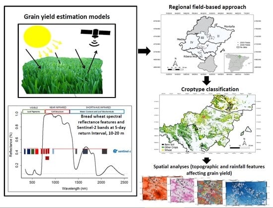
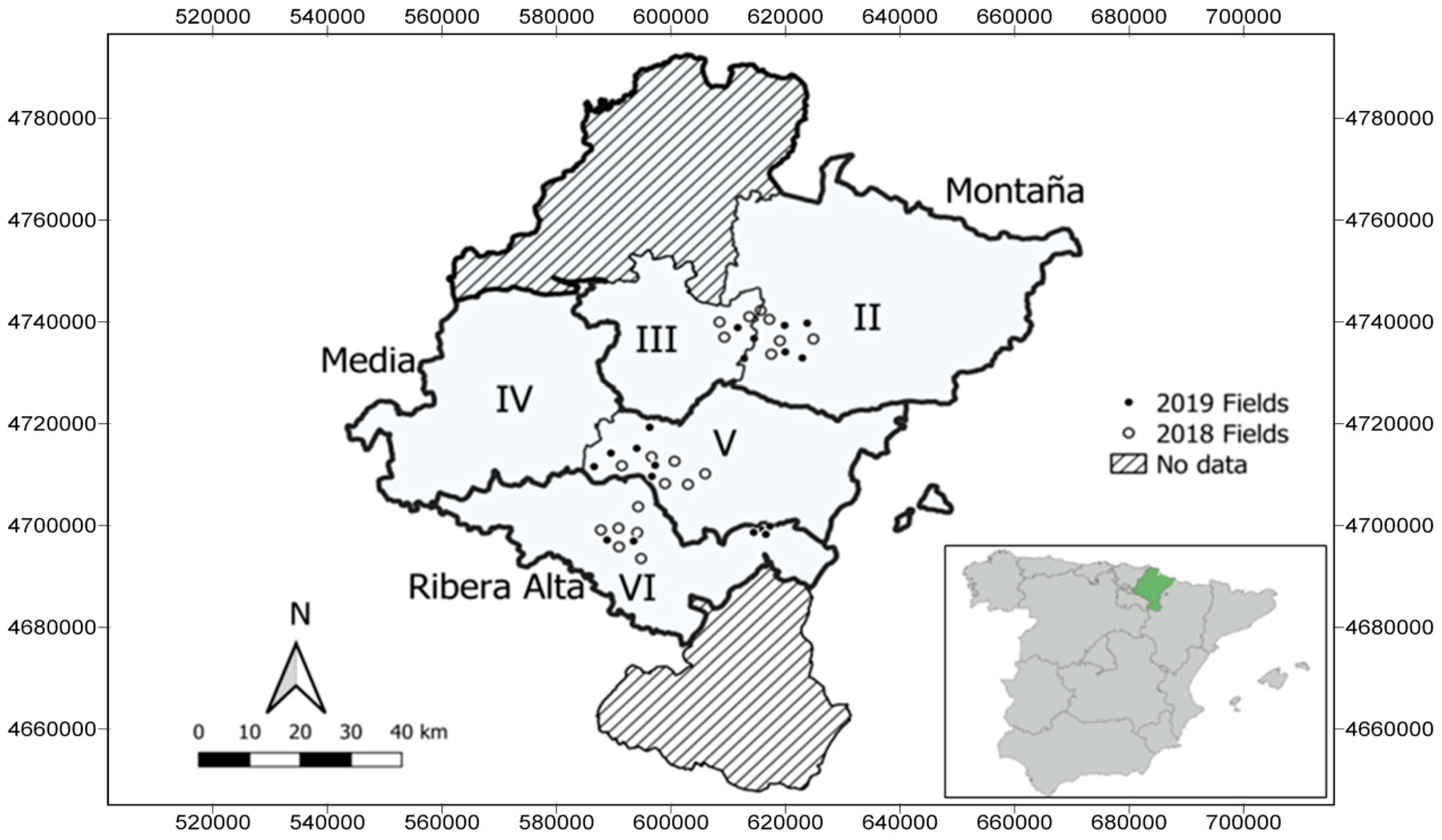
Field-level yield data for training and validation is difficult to obtain as it is often collected in sample plots (crop cuts) or obtained from governmental regional/district level datasets. The objective of this study was to use actual field-level grain yield data in coordination with the local farmers in order to develop empirical models for predicting bread wheat grain yield at the field-level using European Space Agency (ESA) Sentinel-2 imagery in Navarre (Northern Spain). We also aimed to explore different spatial factors influencing wheat grain yield regionally. In order to achieve these objectives, we developed a combination of techniques to take maximal advantage of the still novel aspects of the recent full operationality of Sentinel-2 a + b constellation in terms of its temporal, spatial, and spectral resolution. We aimed to maximize the benefits of improved Sentinel-2 temporal resolution by matching satellite data with phenology over a diverse geographical region. Increased spatial resolution improvements were used for an adequate accuracy of areal crop estimates, and also used for improving empirical models with zonal statistical summaries (maximum, minimum, mean, and median) that take advantage of the increased number of total pixels per field in small- and medium-scale agricultural parcels. We also took advantage of the improved spectral characteristics, which are pivotal for a refined crop monitoring, with stepwise multilinear equations to explore zonal statistic combinations of ten different vegetation indices calculated per field. Furthermore, wheat-growing parcels in the region were mapped using the random forest classification algorithm and the most suitable Sentinel-2 spectral reflectance bands. Finally, the model developed for estimating grain yield was applied to each of the classified wheat parcels, and then spatial topographic factors (aspect, altitude, and slope) and rainfall effects on grain yield were investigated for their correlations with grain yield across all bread wheat fields for the entire Navarre region of Spain.

2. Materials and Methods

2.1. Data

2.1.1. Study Site

The study area is the Charted Community of Navarre in Northern Spain. Navarre’s sub-regions are divided into agrarian zones, as shown in Figure 1. Montaña is divided into two zones, as well as Media, while Ribera Alta is one zone by itself. The region of study is very diverse and incorporates several of the most common Spanish agro-climates, with rainfalls averaging from 800 to 1000 mm in the northern areas, between 800 to 300 mm in the middle and under 300 mm in the southern areas. The two most cultivated rain-fed winter crops are bread wheat (Triticum aestivum L.) and barley (Hordeum vulgare L.), which occupy the 83% of winter croplands in Navarre [34]. The cultivation of bread wheat is ubiquitous throughout Navarre, except for the Northern Pyrenean and Atlantic areas with more rugged topography, lower temperatures, and excess precipitation, as well as in southern bottom-end semi-arid areas, which are too arid and thus unsuitable for growing commercially rain-fed wheat. The majority of crop lands are middle to small holdings, which has made them previously difficult to map adequately with satellite data.
The region has an advanced agricultural intensification with high agronomical standards in terms of cultivation (e.g., certified seeds and widespread access to fertilizers). The regional three-season crop rotation guidelines for bread wheat are fallow, followed by fava beans, oat or sunflower, and bread wheat again in the following third season. Rotation practices are widely encouraged by agrarian institutions. Wheat is sown between the middle to the end of October depending on the agrarian region within Navarre, harvesting happens between the end of June and the middle of July. Grains are mainly commercialized to markets through various agrarian cooperatives distributed throughout the region.

2.1.2. Field Data

During two growing seasons (2017–2018 and 2018–2019), 39 farmer-managed agricultural fields growing either the Marcopolo or Camargo varieties of bread wheat were studied. The fields were different for each season. Both Marcopolo and Camargo are winter, long-cycle genotypes. For both years, 15 fields were selected in the northern region (Montaña), 12 in the middle region (Media), and 12 in the southern region (Ribera Alta) (Figure 1). In 2017–2018 growing season, 8 fields were located in Montana, 6 in Media, and 6 in Ribera Alta; whereas in 2018–2019 season, 7 fields were located in Montana, 6 in Media, and 6 in Ribera Alta. Periodical field visits were programmed in order to follow the phenological stage of the crop and report any specific growth-related issues. As reported by the farmers the analyzed fields received a basal fertilization with either superphosphate 45% or pig slurry, top-dressing fertilization was also applied with granulated urea at the majority of fields. In the Montaña region wheat was sown around the 20th October, in the Media region around the 28th October, and in the Ribera Alta around the 30th October. The harvest was collected around the middle of July in Montaña and during the first week of July in Media and Ribera Alta. The grain yield (Kg·ha−1) per field was reported to the researchers by the participating farmers and standardized in terms of humidity.

2.1.3. Meteorological Data

Temperature data, in order to estimate the crop phenological stages through the calculation of growing degree days (GDD) in zones II, V, and VI, was obtained from 30 openly accessible regional government meteorological stations (www.meteo.navarra.es/estaciones), shown in Figure 2. Rainfall data was also obtained from the same 30 meteorological stations distributed throughout the three agricultural zones under study. The GDDs for each of the two varieties for rain-fed management in Navarre is shown in Table 1 [35].
Following average minimum and maximum mean temperatures of the 30 stations at the three zones, the accumulated GDD was calculated (Equation (1)) following calculations by Arnold [37] to estimate zonal phenological dates for 2018 and 2019 seasons. The reported dates that adjust to the phenological stage regarding GDD (Table 1) are reported in Table 2; as Camargo and Marcopolo had slightly different GDD for each stage, the average of both was considered to estimate the zonal phenological date.
G D D = j u n n o v T m a x + T m i n 2 T b a s e
where GDD is the growing degree days, j u n n o v indicates the sum throughout the season, November to June, of daily maximum and minimum temperatures (Tmax and Tmin) divided by 2, minus the base temperature, which in this case was considered to be 0 °C.

2.1.4. Sentinel-2 Imagery and Phenology

The specific dates of Sentinel-2 images for 2018 were selected as those closest to the estimated phenological date (regarding GDD calculations) per zone as detailed in Table 2 and with the minimal cloud cover thresholds; the specific Sentinel-2 images used in this study are shown in Table 3. The Sentinel-2 a + b satellite constellation’s combined global coverage every 5 days enables this level of phenology matching for the first time ever since its second satellite was launched in 2017.
Sentinel-2 multispectral bands (Table 4) were downloaded from Copernicus Open Access Hub (https://scihub.copernicus.eu/). Despite the high 5-day temporal resolution of Sentinel-2 a + b constellation, some images were discarded due to the image-wide cloud cover areas exceeding 40%. Four Sentinel-2 tiles cover the region under study. The images were downloaded for the 2018 (15-03, 30-03, 14-04, 24-04, 09-05, 19-05, 24-05, 03-06, 18-06 and 23-06) and 2019 (15-03, 20-03, 25-03, 30-03, 09-04, 29-04, 09-05, 14-05, 08-06, 18-06 and 28-06) seasons. Images were downloaded as an L1C product and were corrected to level 2A using the Sen2Cor tool on SNAP (Sentinel Application Platform), obtaining Bottom-Of-Atmosphere (BOA) and cirrus corrected reflectance images. Moreover, a cloud and cloud shadow mask were also applied with this tool.
From the Sentinel-2 multispectral data bands (Table 4), the following spectral reflectance vegetation indices (VIs), which are simple mathematic combinations of spectral bands, were calculated: the chlorophyll index green (CI green) and the chlorophyll index red edge (CI red edge), related to chlorophyll content [38]; the normalized difference water index (NDWI), related to water content [39]; the modified soil-adjusted vegetation index (MSAVI) [40] and the optimized soil adjusted vegetation index (OSAVI) [41], associated with vegetation cover; and the renormalized difference vegetation index (RDVI) [42], the ratio vegetation index (RVI) [43], the modified simple ration (MSR) [44], the normalized difference vegetation index (NDVI) [45], and the green normalized difference vegetation index (GNDVI) [46] sensitive to biomass (Table 5).

2.1.5. Polygons

The agricultural parcels delineations were obtained from Sistema de Información Geográfica de Parcelas Agrícolas (SIGPAC), a Spanish governmental application (http://sigpac.mapa.gob.es/) that allows identifying specific declared agricultural fields subjected to Common Agricultural Policy (CAP) subsidies. GPS coordinates were recorded to delineate the 39 fields used for training and validating the grain yield model. Crop type points were coordinated in fields throughout the three zones (Figure 3) by obtaining GPS coordinates from each of the classified types (wheat, bare soil, and other crops). The whole regional agricultural parcels polygons were downloaded for the attributes herbaceous crops and rain-fed for the three agrarian areas under study within Navarre. Furthermore, fields were 10-m-buffered with the ArcGis Pro 2.3.0 buffer tool in order to reduce edge effects.

2.2. Models and Analysis

2.2.1. Grain Yield Estimation

At each of the three studied phenological stages (tillering, heading, and ripening), the previously described vegetation indices were calculated per field on ArcGis Pro 2.3.0 using the downloaded Sentinel-2 imagery. Four different statistical summary extractions of each vegetation index (maximum, minimum, mean, and median) were obtained for each field at each different phenological stage, considering the regional differences outlined in Table 2 and Table 3. Mean and median were calculated with the closest available images to the phenological stage using zonal statistics, while minimum and maximum were respectively the averages of the lowest and highest pixel values between the two closest dates to the phenological stage. These calculations were performed on ArcGis Pro 2.3.0 and Microsoft Excel. First, the Raster to Point and Spatial Join tools on ArcGis were used in order to list, per field, all the pixel values; second, with the corresponding attribute tables the maximum and minimum vegetation indices pixel values between the dates were calculated with Microsoft Excel. Finally, the maximum and minimum were calculated on the points’ attribute table were converted into two rasters in ArcGis in order to perform zonal statistics and obtain maximum and minimum averages per field over the specific periods. Pearson regressions against grain yield were calculated on R studio (“cor.test”) for each phenological stage and summary (min, max, mean, and median). Following this, in order to find the combination of the best vegetation indices and statistical summary to estimate grain yield, multilinear stepwise regressions were studied at the most suitable phenological stage in R Studio (library “MASS”). The selected best model was chosen on the basis of Akaike Information Criterion, computed with the stepAIC function from the MASS library. The normal distribution of residuals and collinearity of the independent variables were studied with the library “olsrr”, the variance inflator factor (VIF) was measured as it is an efficient method to asses collinearity [47,48,49], which strongly limits stepwise selection method. Furthermore, the residuals normality Shapiro-Wilk test was calculated.
The 39 monitored fields were separated into two groups, one for training and the other one for validation of the multilinear stepwise equations. The 20 fields from 2018 season were used for modeling and the 19 fields from 2019 were used for validation. For the 2019 season, only one phenological stage, heading, was eventually analyzed, as it appeared to be the most suitable for grain yield estimation (Table 7), with the following images: Montaña, 09-05 and 14-05; Media, 14-05 and 08-06; and Ribera Alta, 29-04 and 09-05.

2.2.2. Crop Type Classification and Regional Per-Parcel Grain Yield Estimation

We performed a pixel-based supervised random forest (RF) classification to differentiate wheat fields from fields of other crops. The classified area was stratified in three zones: II, V, and VI, corresponding to three of Navarre’s agricultural zones shown in Figure 1. Each one located in Montaña, Media, and Ribera Alta areas, respectively. Following Colditz [50] and Noi and Kappas [27], which state that for RF classifications the training sample should correspond to around 0.25% of the total area, 513 points of parcels of the ground dataset in Zone II (33,345 pixels), 927 in Zone V (58,401 pixels), and 1050 in Zone VI (60900 pixels) formed the training dataset. Figure 3 indicates the points of the parcels from which the pixels from the various analyzed classes were obtained. The points collected were classified into three classes: wheat, bare soil, and other crops. As mentioned before, the target classification areas were delimitated with the available rain-fed and herbaceous crops polygons mask from SIGPAC.
Considering that the majority of cropland under study (83%) is either bread wheat or barley, we took advantage of the later ripening of bread wheat in order to differentiate it from other crops. After considering both preliminary results and phenological characteristics, differences between wheat and barley were clearer late in the season. This is a consequence of the shorter crop duration of barley, which makes it reach maturity and change color before wheat. Hence, late season Sentinel-2 images (24-05-2018, 03-06-2018 and 18-06-2018) were used for the classification as the moment of greatest contrast.
Due to their better spatial resolution (10 m) and contrasting capacities in comparison with its other bands, Sentinel-2 B3 (green), B4 (red), and B8 (near infrared) bands were used for the crop type classification. Crop classifications [26,51] and field boundary delimitation [52] were successfully mapped using B3-B4-B8 images in previous studies with Sentinel-2 data. The trained datasets were divided as follows, 2/3 for training the model and 1/3 for validation. The number of trees was 500 [53]. RF classification and object filters were computed with ArcGis Pro 2.3.0. We applied majority voting of the classified pixels within the agricultural parcels (SIGPAC), as field crops are exclusively grown in monocultures in the region of Navarre, which we confirmed during farmer visits. The pixel’s majority from the zonal statistics tool was then used to object filter the classification. With the validation data and the output of classification, a confusion matrix was computed at parcel level in order to obtain classification accuracies. At parcel level, the Fscore of each class was calculated with the Equation (2), where PA refers to producer’s accuracy while UA refers to user’s accuracy.
F s c o r e = 2 P A U A P A + U A
The most suitable multilinear stepwise regression model was extended into all the classified parcels of bread wheat in order to estimate grain yield per field for the three agricultural sub-regions. The resulting wheat cropland and grain yield average per zone were compared to the Navarre regional government’s official statistics (www.navarra.es).

2.2.3. Rainfall Interpolation and Topographic Models

A 2 m resolution digital elevation model (DEM) was obtained from Navarre’s regional Government at ftp://ftp.cartografia.navarra.es/. The downloaded tiles were mosaicked and slope and aspect were calculated from the DEM using the slope and aspect tools.
The sum of the accumulated rainfall (mm) during the wheat growing season, from November to May, at every station was gathered in a georeferenced-points dataset. This dataset was used to interpolate rainfall using two strategies: inverse distance weighting (IDW) and kriging. All DEM, topographic feature and subsequent GIS processing were completed on ArcGis Pro 2.3.0.

2.2.4. Ordinary Least Square and Geographically Weighted Regression

The ordinary least square (OLS) was used in the first term to explore the relationship between grain yield and the explanatory variables. In OLS the existence of local variation is not taken into account in the regression, hence the regression coefficient remains constant for each variable (Equation (3)).
yi = β0 + ∑k βk xik + εi
where yi is the dependent variable (grain yield), β0 is the intercept; βk is the coefficient of the independent variable (xik) and the random error is εi.
Alternatively, GWR 4.0 software, developed by Nakaya et al. [54], was used. A geographically weighted regression (GWR) model was also calculated in order to explore the relationship between grain yield and the explanatory variables (Equation (4)) taking into account the spatial factor, which is an essential feature when dealing with spatial heterogeneity, something that is especially central to the objectives of this study. GWR uses the least square method given the location as a weighting factor. The optimal bandwidth, namely the optimum number of neighbors, was determined by the Akaike Information Criterion (AIC). A multiple comparison of AIC to find the best bandwidth (the one with the lowest AIC) was computed. For OLS and GWR comparison, an ANOVA was performed to compare the accuracy of both levels. Furthermore, for both OLS and GWR, the spatial autocorrelation (Moran’s I) of residuals were tested.
yi = β0(µi,vi) + ∑k βk(µi,vi) xik + εi
where yi is the dependent variable (grain yield), (µi,vi) are the coordinates (x,y) at the location i, β0 is the intercept, βk is the coefficient of the independent variable (xik) at the specific weighted location, and εi is the random error.
A geographic variability test was performed in order to determine if the explanatory variables were spatially heterogeneous. In order to do so, two models were developed, one that considers all of the variables (slope, altitude, height, and rainfall) to be spatially heterogeneous, and on the other hand one that considers all of the variables to be spatially homogenous. If the variables were indeed spatially heterogeneous determinants of grain yield, i.e., if the coefficients varied significantly in space, then the AIC size of the second model should be larger and result in a negative diff-criterion value for this test (GWR4 manual) [55].

3. Results

3.1. Grain Yield Estimation

In Table 6 we show the Pearson’s correlation between the calculated vegetation indices and the actual grain yield at the three studied phenological stages (tillering, heading, and ripening) for the various extracted zonal statistics (min, max, mean, and median). The correlations were substantially higher at heading in comparison with tillering and ripening. The resulting correlations against grain yield were similar among the chlorophyll content, water content, vegetation cover, and biomass-sensitive vegetation indices, with no obvious results to determine better correlating indices with the Pearson’s correlation. While at heading the correlations averaged between 0.79 to 0.84 for the mean, 0.76 to 0.84 for the median, 0.72 to 0.81 for the minimum, and 0.82 to 0.84 for the maximum, at tillering the results were between 0.41 and 0.74 for the mean, 0.40 and 0.71 for the median, 0.38 and 0.63 for the minimum, and 0.43 and 0.65 for the maximum. Regarding ripening, the correlations yielded between 0.32 and 0.49 for the mean, 0.31 and 0.49 for the median, 0.38 and 0.45 for the minimum, and 0.34 and 0.45 for the maximum. Furthermore, the statistical significance of the correlations at heading was greater than that at both tillering and ripening, which demonstrated lesser (<0.05) or no significance differences in the majority of the cases.
At heading, the results from the multilinear stepwise regression (Table 7) show the most suitable combination of vegetation indices in order to estimate grain yield. In this sense, the best-suited equation uses minimum averages of MSAVI pixels and maximum averages of RDVI pixels. VIF was 2.16 for both variables. The histogram of the residuals is shown in Figure A1 in the Appendix A together with the Shapiro-Wilk normality test results, the null hypotheses of which assumes that the data is normal while the alternative assumes it is not. The p value of the test was 0.297 and the statistic 0.982.
The resulting multilinear stepwise equation (Table 7) was tested at heading for the studied fields for the following year 2019 using the corresponding calculated vegetation indices and summary statistics. The equations worked accurately as shown in Figure 4, with an R2 of 0.83 (RSE = 733.1 kg·ha−1).

3.2. Crop Type Classification

The overall classification accuracy reached 86.55%, 89.32%, and 83.14% for the II, V, and VI zones, respectively (Table 8). Wheat was well-mapped at the three classified sites with an Fscore of 88% at the agrarian sub-regions II, 91.90% at zone V, and 84.05% at zone VI. On the other hand, bare soil was reliably classified with an Fscore of 91.43% at zone II, 93.26% at zone V, and 84.06% at zone VI. The class “other crops” was the least well classified, the corresponding Fscores at the three areas where 78.15%, 78.26%, and 81.82% for the zones II, V and VI, respectively. Figure 5 shows the crop type classified map.
The estimated grain yield average for zone II corresponded to 103% of the official data, while zone V and VI correspond to 95% and 94%, respectively (Table 9). Regarding wheat crop land, the classified wheat field area can be an indicator of the crop type area. In this sense, the estimated wheat crop land area for the whole region corresponded to 85.77% of the estimate in the official statistics. Regarding each zone, the surface corresponded to 81.41%, 81.15%, and 123.16% with the zones I, V, and VI respectively. Regarding zone VI, the estimated wheat cropland was overestimated if compared with official statistics, while the opposite happened at sites I and V. We trust the area estimation indicator as the polygons used for the object-filtering are official trusted vectors, as well as the mask used for the classification itself. All Spanish cereal producers are required to declare their croplands, and thus the polygons used in this study should be fairly accurate.

3.3. Topographic Features and Rainfall Effects on Performance

OLS and GWR are both models that seek to explain the relationship between a dependent variable, in this case the calculated grain yield at all the classified wheat parcels, and explanatory independent variables, topographic features (aspect, slope, and altitude), and rainfall for this study. Table 10 presents GWR as the most suitable model for explaining these effects. In this case AIC, sigma and both R2 and adjusted R2 improved with GWR in comparison with OLS for the three zones (II, V, and VI) (Table 11). For instance, OLS yielded an adjusted R2 of 0.05, 0.06, and 0.07 for zones II, V, and VI respectively. Meanwhile, for the statistically significant (p < 0.05) independent variables (rainfall and altitude in zone II; rainfall, slope, and altitude in zone V; and rainfall, slope, and altitude in zone VI) OLS can explain a 5%, a 6%, and a 7% of grain yield variability at each zone (II, V, and VI). On the other hand, GWR presents an adjusted R2 of 0.20, 0.11, and 0.20 for zones II, V, and VI respectively; therefore 20%, 11%, and 20% of GY variability at each zone can be explained with GWR. The local R2 of each wheat field is shown in Figure 6. Furthermore, in Table 10, the ANOVA results support significant improvement (p < 0.05) when using GWR in all the three studied zones compared to the global model (OLS). The GWR model explains the effects of topographic factors (aspect, altitude, and slope) and rainfall on grain yield significantly better than the OLS model for all three zones by adding information on the spatial variation of grain yield with these local phenomena.
The autocorrelation test of both GWR and OLS for the three zones (Table 12) presents Moran’s I values closer to the expected for GWR in comparison with OLS. The complete spatial randomness of GWR residuals was accepted as the p-value is not statistically significant, making the null hypothesis, that there is not significant spatial autocorrelation, correct. In contrast with this, p-value is statistically significant for OLS and therefore shows spatial autocorrelation of OLS residues.
Regarding the rainfall interpolation, kriging interpolation outperformed IDW (RMSE = 91.90 mm and 105.08 mm respectively), hence the previous was used. Grain yield correlated positively with rainfall, namely when rainfall increased, so did grain yield. Although in GWR models the regression coefficients vary locally, the fact that in zone II the mean coefficient is 13.87 (Table 11) suggests the strong effect of the rainfall gradient distribution on wheat grain yield in this northern area. Regarding rainfall at the southern region (Zone VI), the mean coefficient is also positive and relatively high, 12.32 (Table 11). Meanwhile, the mean regression coefficient in zone V was lower at 1.73. Concerning the topographic variables, they were spatially heterogeneous except for aspect in the middle zone.

4. Discussion

Testing the applicability of empirical vegetation index models in different years of data allows for evaluating the reliability and reproducibility of that model through time. In this case the stepwise multilinear model split between the training dataset, season 2018, and validation dataset, season 2019, revealed the efficiency of this approach for at least a two-year period in Navarre. This is uncommon, as generally such empirical models are developed and validated with same-year data [16,21], something that likely happens due to the difficulty to obtain data from various growing seasons, and thus gives robustness to the techniques and analyses that we have presented here.
The full operationality of Sentinel-2 constellation reached in 2018 allowed focusing on phenological stages thanks to its improved frequency, as the results presented here show. Until this recent date, phenology-based grain yield prediction was unlikely to be assessed with alike satellites (i.e., Landsat 8). Our results suggest that heading is the most suitable phenological stage in order to study empirical relations of vegetation indices with grain yield for rain-fed wheat in Navarre. This is consistent with other ground spectral measurements for estimating wheat grain yield under rain-fed conditions as reported by Fernández-Gallego et al. [56]. Moreover, this stage was also found optimal for grain yield prediction with proximal remote sensing (i.e., UAV) and equivalent growing conditions [57]. We argue that the results here obtained showed that focusing on phenology for grain yield estimation is now possible using Sentinel-2 imagery and not only applicable with ground and proximal sensing. Furthermore, the combination of climatic (i.e., temperature, growing degree days) and satellite data has resulted in an adequate approach for estimating phenology, as previous studies have suggested [58,59], and wheat grain yield.
The minimum average of pixel values at heading stage of MSAVI and the maximum of RDVI provided the most optimal combination of vegetation indices in the stepwise multilinear regression produced in this study. The improved features of Sentinel-2 regarding spectral and spatial resolution have allowed increasing the VIs able to be calculated and the most optimal statistic summary, which with coarser spectral and spatial resolutions would be very limited. The improved capacities of these indices could be explained due to the reduced soil background influences, regarding MSAVI, and, as detailed by Rougean and Breon [42], the capacity to minimize background reflectance effects of RDVI. In this case, MSAVI together with RDVI show the ability to maintain sensitivity to total vegetation biomass for fully developed canopies corresponding to heading, while other vegetation indices might be saturated at this phenological stage. These vegetation indices have already been successfully correlated with wheat performance using remote sensing data. In the scientific literature, we find examples of RDVI, which is used for green biomass estimation as it is sensitive to vegetation coverage [60] and has also been successfully used in empirical models estimating wheat yields [61]. Around the phenological stage of heading, Bao et al. [62] reported a correlation of 0.79 (R2) between RDVI and wheat yield, while Zhao et al. [63] found a correlation of 0.76 (R2), which show the relative high correlation ability of RDVI with wheat yield. Examples are also available for MSAVI, which has shown relative high correlation with wheat yields [64,65]. Regarding the goodness of the model, the selected vegetation indices showed absence of collinearity, as a VIF of 2.16, obtained for both cases, was lower than the collinearity threshold value of 10 [
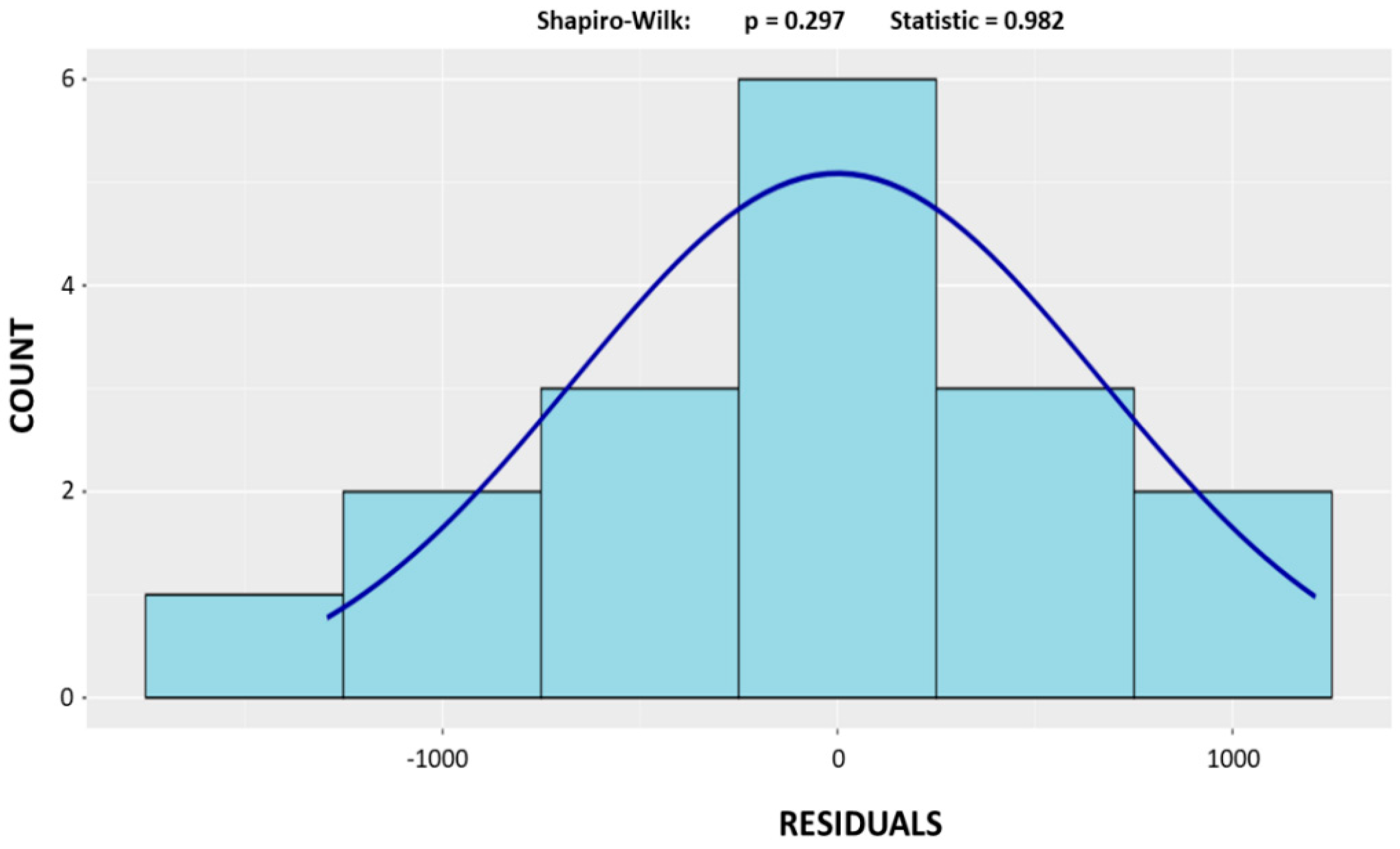
66]. Moreover, the normality of the residuals was assumed, as the Shapiro-Wilk test p value was over 0.05 (0.297) and the null hypotheses, which assumes that the data is normal, was accepted. The plot of residuals also suggested it as shown in Figure A1 of Appendix A.
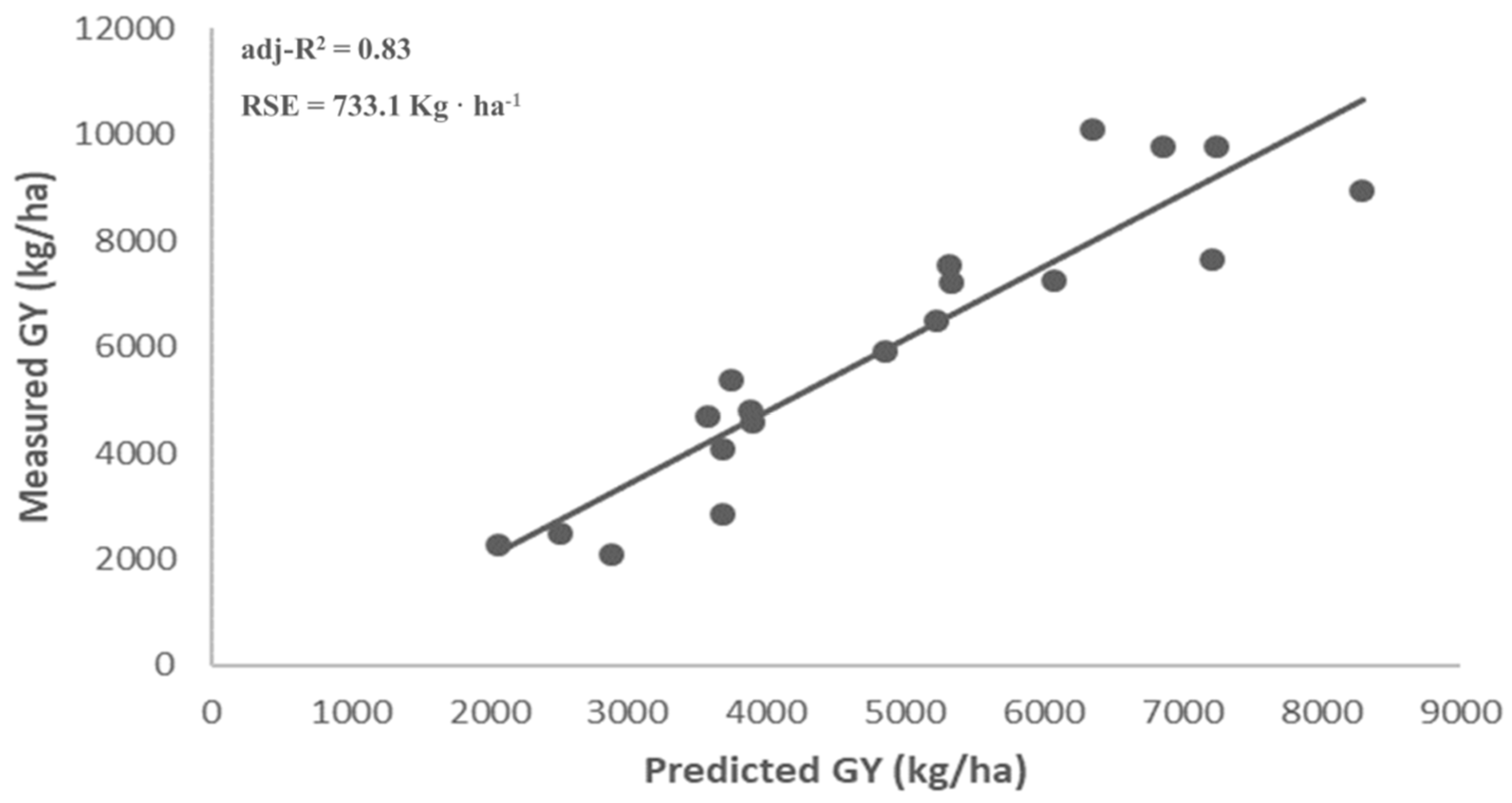
The fact that maximum and minimum pixel value averages were the most suitable statistical summary combination shows that, for studying grain yield, exploring crop canopy evolution through time may provide an improved output in comparison with single date image data. However, it shows that focusing on the phenological period of heading can provide relatively higher correlations with grain yield, explaining 83% of variability in this case. Namely, segregating phenological periods is a a useful approach in order to calculate empirical grain yield estimations in contrast with following whole season pixel values without explicitly considering phenological periods itself. Estimating the phenological stage with the GDD and focusing on the specific period, heading in this case, eases processing demands and yields accurate results, while clearly diminishing costs. Sentinel-2 spatial resolution allows for the fine evaluation of the statistical summaries and consequently more precise estimations.
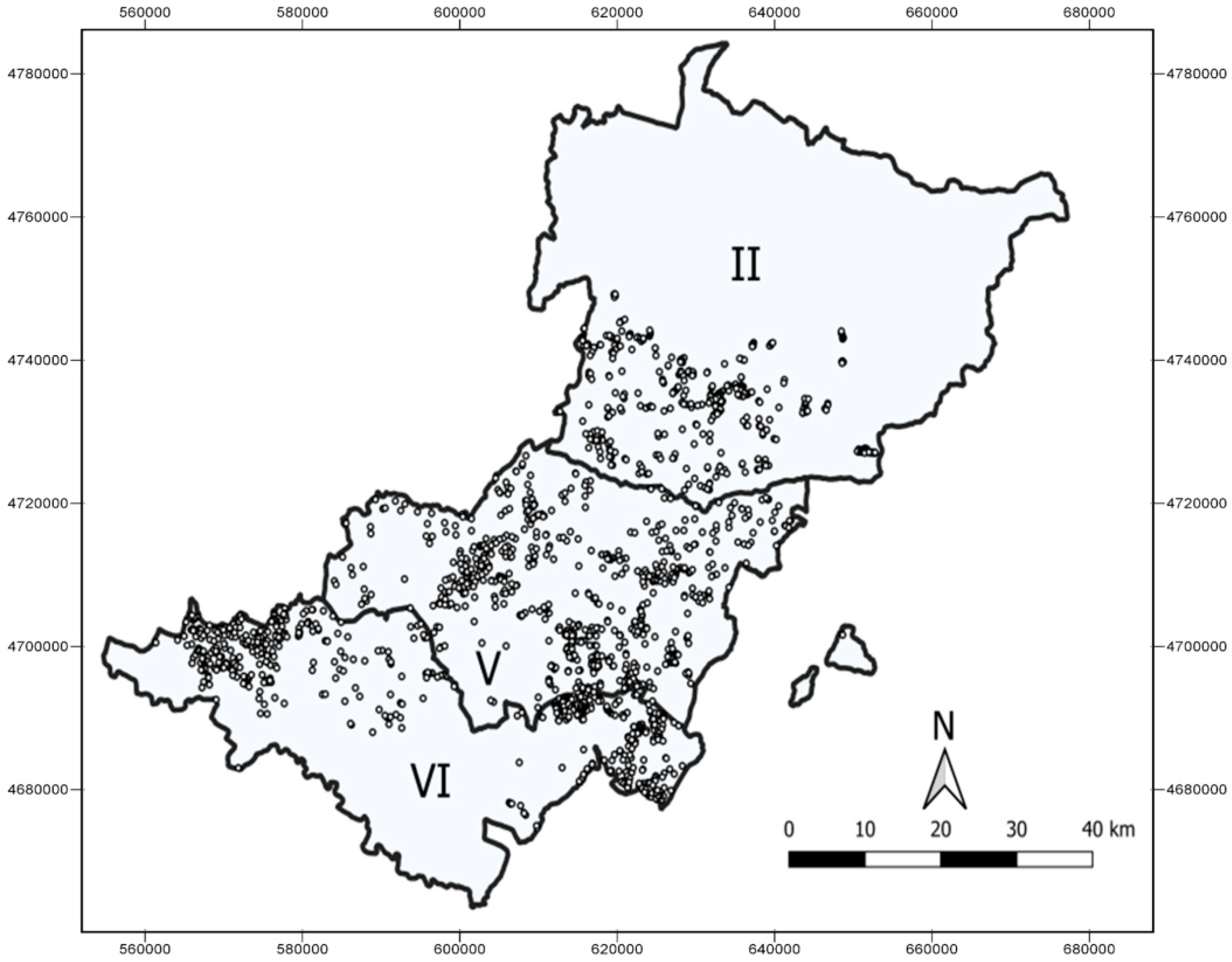
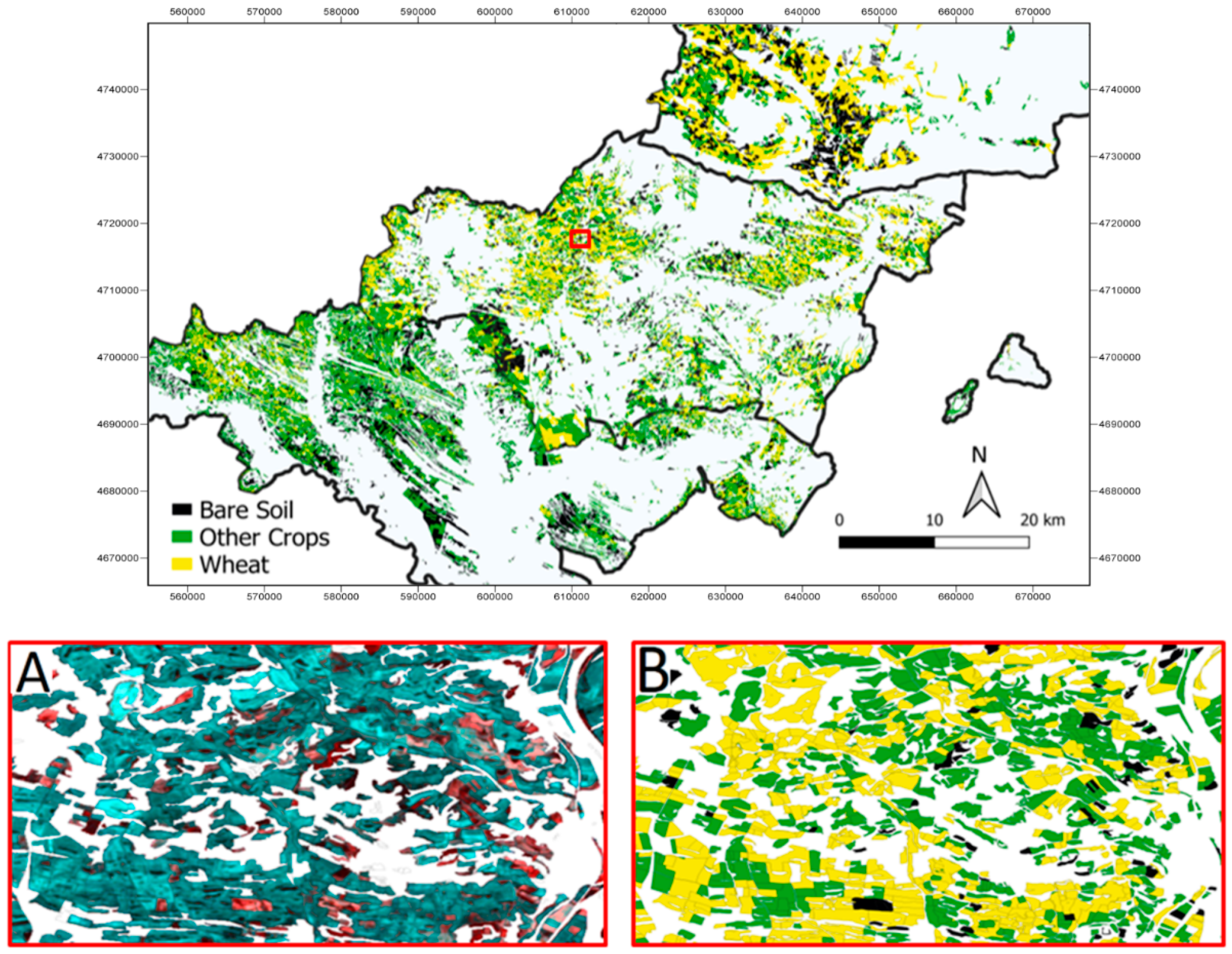
Using late-season imagery in order to take advantage of barley’s earlier senescence proved to be efficient for wheat crop land classification, again, taking maximal advantage of the S2 return interval temporal frequency to identify the optimal date for the separation of like cereal crops. Our results are congruent with the Navarre regional government’s official statistics, as Table 9 demonstrates. The average grain yield obtained after applying the grain yield stepwise equation from Table 7, for all of the classified wheat fields, showed similar results with official (i.e., after harvest) grain yield averages. Sentinel-2 spatial resolution allowed accurate mapping and estimation of grain yield, while other satellites would not have yielded such precise results regarding field delimitations, for instance. The grain yield estimation model was applied to the wheat classified parcels without considering genotypic differences within the region (both concerning classification and grain yield modelling issues) due to the fact that for the 2017–2018 season 80% of the fields across the whole of Navarre used either Camargo or Marcopolo [67]. Therefore, a general wheat genotypic homogeneity was supposed in the whole region.
In order to be able to use the yield estimation based on spectral data from Sentinel-2 to estimate the yield across the entire study area, it is necessary to also develop a pixel or better field-level image classification. The slightly lower Fscore of wheat classification accuracy in the Ribera Alta southern sub-region might be due to the limited surface area devoted to this crop type in comparison with the other two sites—a higher difficulty in accurately classifying wheat fields was observed with 13 misclassifications with a proportionally smaller number of ground data points for wheat at this site (Table 8). Moreover, it could be a consequence of the smaller size of the fields in this southern zone. Bare soil did present substantial misclassification with “other crops” in this southern zone; this likely occurred due to the major presence of barley in zone VI and the earlier senescence it features, especially considering that this zone is substantially drier. Relevant misclassifications happened with wheat and bare soil in all of the three zones. Unfortunately, ground reference points in which the cultivar was specified were only obtained for wheat, the other available ground points could not be specified among the other cultivated crops, namely barley and other minor crops such as oats were not well differentiated. Despite targeting wheat crop lands, specifically classifying each of the various crop types in the region could have improved the classification results overall. Nonetheless, the lack of this exact information did not jeopardize the classification of only the wheat crop lands too much, which showed relatively high Fscores for all of the zones and was the central aim of this study.
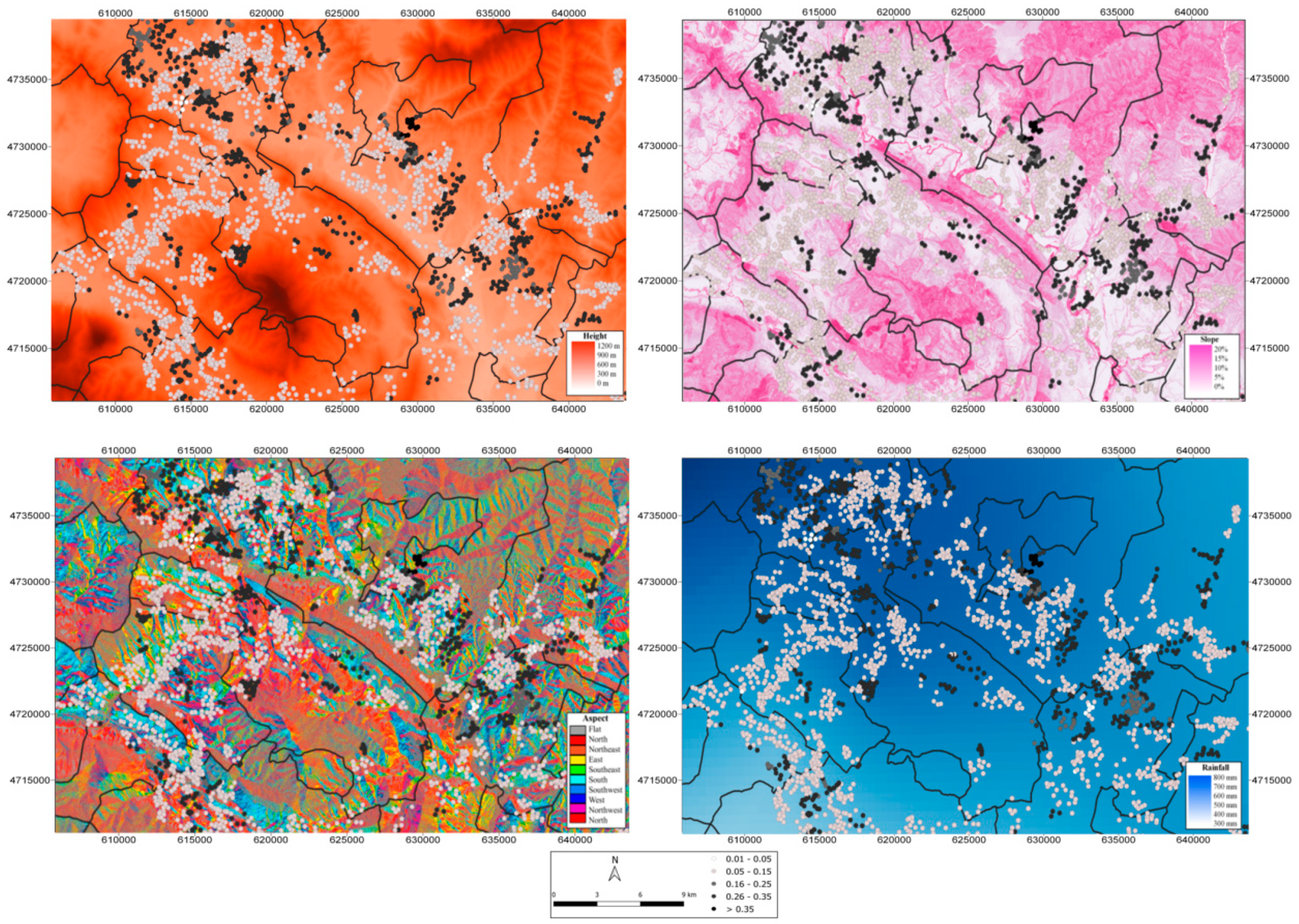
Topographic features and rainfall together accounted for an average of 11% to 20% of the observed spatial variation in grain yield in Navarre; this percentage range is consistent with other studies dealing with these factors. Regarding topography effects on wheat at the field level in central Europe, slope and altitude have been estimated to account for an average of 5% to 42.5% variation in grain yield [68], meanwhile in North America those same topographic attributes were estimated to account for an average of 39% to 65% of the variation in grain yield [69]. Moreover, Basso et al. showed that in the Mediterranean context aspect, altitude, and slope are directly linked with wheat grain yield [70] and that rainfall distribution is a major limiting factor for wheat yields [71]. It has been observed that topographic features affect grain yield more dramatically in dry years or in areas with naturally irregular rainfalls (i.e., Mediterranean rain-fed wheat croplands) [72], which explains the relatively wide range of variability of the rainfall and topographic effects on grain yield in this study as well as in the scientific literature. Thus, an increased effect of topographic features might be expected in Spanish wheat agrosystems in a climate change scenario, and these features consequently deserve attention. In this sense, the results of this study demonstrate novelty as the relations between topography and grain yield found in the scientific literature have been, on the one hand, studied in few or single fields [73], presumably due to the difficulty in obtaining precise grain yield predictions for multiple fields from both traditional methods (i.e., time consuming field-work) and from remote sensing techniques (i.e., access restrictions or coarser resolutions to correlate with grain yields and delineate fields). On the other hand, when focusing on regional-scale topographic and climatic data, previous studies have defined suitability zones solely within the agroecological landscape [74,75,76]; none have completed an estimation of the effects of those factors directly on grain yield. We here took advantage of both topographic and climatic data of Navarre, Spain to explore the potential effects on grain yield in various regions, while estimating precisely the grain yield per field at a regional level using to the best of our advantage all of the Sentinel-2 improved characteristics. We believe that studying climatic and topographic impacts on grain yield at a larger scale can provide new insights that in turn will be of interest for managing croplands systemically while advancing towards improved agroecological landscape assessments.
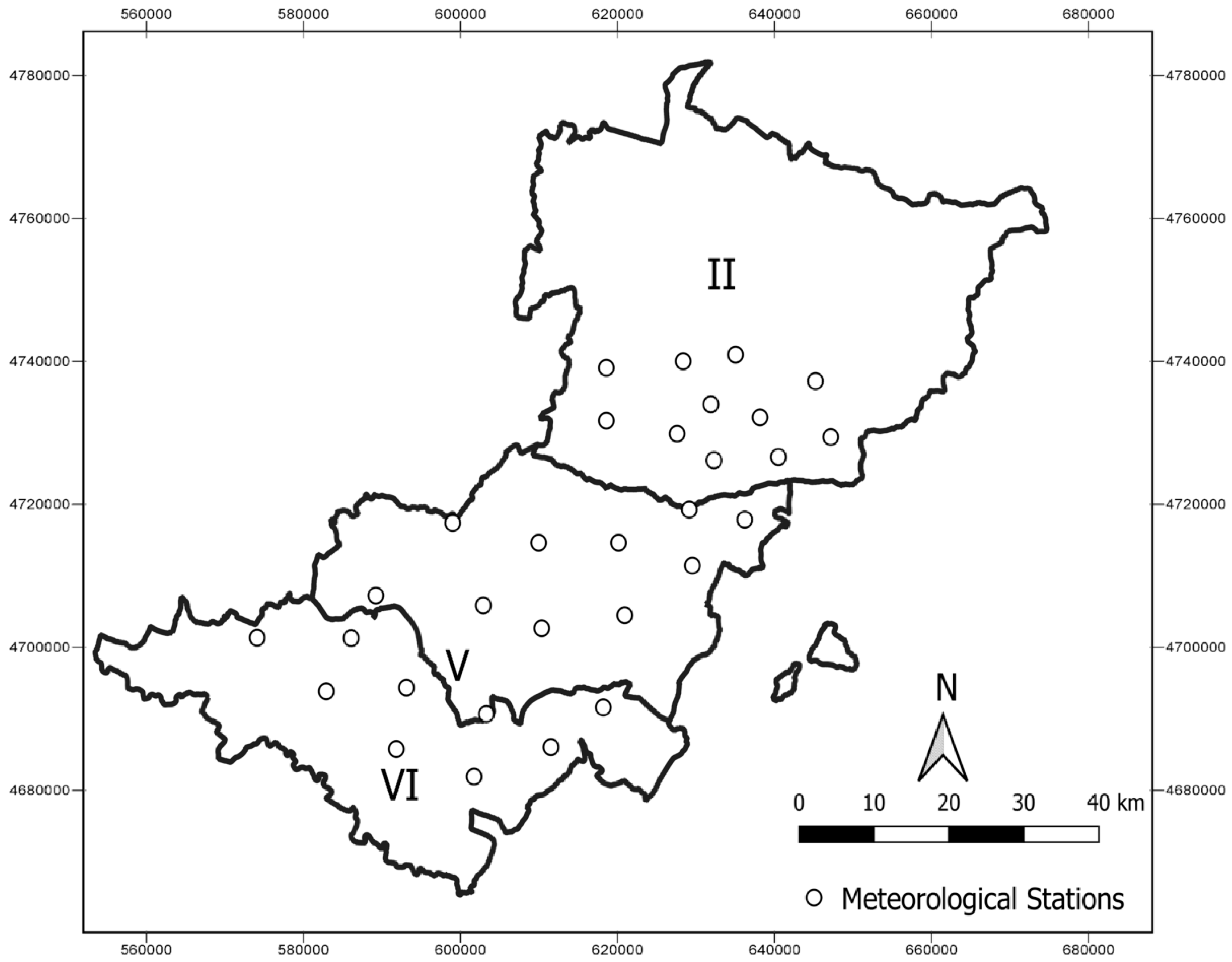
Regarding the previously-mentioned GWR results, approximately 80%, 89%, and 80% of grain yield variability are yet to be explained in each region respectively, as the tested variables cannot explain the whole of the variability. Factors such as soil type, evapotranspiration, radiation, and fertilization or farming practices, among others, could not be evaluated with the remote sensing techniques employed in this study, and might help to explain the remaining variability. Be that as it may, the mean coefficient of regression is positive for rainfall at all three zones. This suggests a relatively strong effect of the rainfall gradient distribution on wheat grain yield in the northern zone. This might be explained with the varying precipitation patterns of the area due to the rugged topography and the numerous valleys that the area includes and that may consequently affect wheat grain yield. Regarding zone VI, the result links the drier features of the southern climate and its positive strong dependence on rainfall.
In zone II, the slope showed a negative coefficient or inverse relationship (the steeper the terrain the lower the GY), while altitude and aspect were positive, hence suggesting that southern-oriented fields at higher altitudes experienced improved performance for that season. Regarding the middle zone, the regression coefficient for the slope was also negative, while the altitude coefficient was positive. In zone VI, the slope and altitude regression coefficients were negative, while aspect was positive. This suggest that at this site that grain yield decreases the higher and steeper the parcel is; while orientation, towards the South in this case, affects grain yield positively. The lower adjusted average of R2 results in zone V suggest only a moderate influence of the tested factors in comparison with the northern zone II and southern zone VI, agricultural areas. This might be due to the milder weather with sufficient rainfall, in comparison with the southern zone, and the fairly flatter ground in comparison with the rugged northern zone.

5. Conclusions

We believe that Sentinel-2′s improved temporal frequency benefitted the grain yield prediction models by adapting to phenology across ecozones in the geographically diverse region of Navarre and improved the spectral separation of bread wheat from other crop types by using precisely timed images at a moment of phenological differences. The improved Sentinel-2 spatial detail was also optimally harnessed by capturing field level variability with the use of zonal statistics as model input parameters, and contributed to improving total estimates related to both yield and crop types. Furthermore, the use of field-level grain yield data for both training and validation of the wheat grain yield estimation model proved to be an efficient approach. The matching of crop type classification and field-level grain yield estimation models are scarce in the scientific literature, as often studies either focus on classification [23,24,25,26] or grain yield estimation [17,18,19,20,21,22] alone. Notwithstanding, the combination of both as presented in this study provided improved data for a more robust model (i.e., comparison to official cropland area and regional yield statistics) and for testing its applicability in actual agricultural contexts. Moreover, another novel aspect that this research addresses is the study of large-scale field-level topographic effects on grain yield, which has not been studied extensively, as single fields or reduced-scale approaches are used in the majority of studies on this topic [73].
In addition, we have applied here various techniques to take maximal advantage of several different types of openly accessible data sources for the Navarre region in northern Spain, where no such study had been previously reported. It is especially relevant, as in 2020 the CAP in the European Union will be reformulated aiming to optimize resources and advance towards an integrated regional management. The CAP accounts for around 30% of the total European budget [77], and member states are responsible of supervising the declared croplands and harvests. The results obtained and the methodology here developed can be easily used and reproduced for both Navarre’s regional government and other European regions with equivalent data availability and frameworks, easing their expensive field works. We here used polygon databases from agricultural fields declared in the CAP subvention system, public topographic and environmental data, as well as European Union and European Space Agency-launched Sentinel-2 openly accessible imagery. Furthermore, we believe that in order to obtain field-level crop yields in actual agricultural contexts, coordination with local farmers is central to this endeavor.
In summary, this research successfully showed the ability of our relatively straightforward and potentially operational method for estimating wheat grain yield at field-level before harvest and determining the spatial factors that influence grain yield. Concerning grain yield estimation, two observations were deemed most pertinent: on the one hand this approach allows grain yield at approximately two months before harvesting (at the phenological stage of heading) to be estimated correctly, and on the other hand, it is applicable across at least a two-season period. The combination of our grain yield estimation model and crop type mapping also achieved accurate results with regards to official statistics. The techniques and models presented can be said to have successfully mapped wheat croplands and calculated regional grain yields. Furthermore, the observed spatial variation caused by topographic features (slope, aspect, and altitude) and rainfall could be attributed to explain on average 11% to 20% of spatial grain yield variation. Additional work is warranted in relation to the other genotype/varietal, environmental, or management (GxExM) factors that may account for regional grain yield variability across local to regional scales, such as those presented here for Navarre, Spain.

Author Contributions

J.L.A and S.C.K. designed and had the original idea of the study. J.S. processed the Sentinel-2 images, mapped the crop types, developed the performance estimation models and analyzed the topographic and rainfall effects on it under the supervision of J.L.A. and S.K. J.G.-T. and I.A. managed the field work in Navarre and organized the datasets. J.S. and S.C.K. wrote the paper.

Funding

This study was supported by the Spanish projects PID2019-106650RB-C21 from the Ministerio de Ciencia e Innovación and the IRUEC PCIN-2017-063 from the Ministerio de Economía y Competividad and by the project “Nuevas aplicaciones de agricultura de precisión para la monitorización del rendimiento del cultivo de trigo en Navarra” from the Government of Navarre, Spain (0011-1365-2018-000213/0011-1365-2018-000150).

Acknowledgments

We would like to acknowledge all the anonymous farmers working with wheat in Navarre that participated in this study. We would also like to thank the anonymous Reviewers for their comments and suggestions, which contributed significantly to the improvement of the revised version of the manuscript. J.L. Araus also acknowledges the support of Catalan Institution for Research and Advanced Studies (ICREA, Generalitat de Catalunya, Spain), through the ICREA Academia Program.

Conflicts of Interest

The authors declare no conflict of interest.

Appendix A

Figure A1. Histogram of the residuals of the stepwise model to assess the normality assumption.
Remotesensing 12 02278 g0a1

References

  1. Calatrava, C.A.; Spiegelberg, P.S.; Díaz, I.B.; Piferrer, S.J. Avances Nacionales de Superficies y Producciones Agrícolas; Ministerio de Agricultura, Pesca y Alimentación del Gobierno de España: Madrid, Spain, 2018. [Google Scholar]
  2. EU Regulation (EU) 1306/2013 of the European Parliament and of the Council on the financing, management and monitoring of the common agricultural policy. Off. J. Eur. Union 2013, 347, 549–607.
  3. Hunt, M.L.; Blackburn, G.A.; Carrasco, L.; Redhead, J.W.; Rowland, C.S. High resolution wheat yield mapping using Sentinel-2. Remote Sens. Environ. 2019, 233, 111410. [Google Scholar] [CrossRef]
  4. Toscano, P.; Castrignanò, A.; Di Gennaro, S.F.; Vonella, A.V.; Ventrella, D.; Matese, A. A Precision Agriculture Approach for Durum Wheat Yield Assessment Using Remote Sensing Data and Yield Mapping. Agronomy 2019, 9, 437. [Google Scholar] [CrossRef] [Green Version]
  5. Spitters, C. Crop Growth Models: Their Usefulness and Limitations. Acta Hortic. 1990, 349–368. [Google Scholar] [CrossRef]
  6. Burke, M.; Lobell, D.B. Satellite-based assessment of yield variation and its determinants in smallholder African systems. Proc. Natl. Acad. Sci. USA 2017, 114, 2189–2194. [Google Scholar] [CrossRef] [Green Version]
  7. Matsushita, B.; Yang, W.; Chen, J.; Onda, Y.; Qiu, G. Sensitivity of the Enhanced Vegetation Index (EVI) and Normalized Difference Vegetation Index (NDVI) to Topographic Effects: A Case Study in High-Density Cypress Forest. Sensors 2007, 7, 2636–2651. [Google Scholar] [CrossRef] [Green Version]
  8. Defourny, P.; Bontemps, S.; Bellemans, N.; Cara, C.; Dedieu, G.; Guzzonato, E.; Hagolle, O.; Inglada, J.; Nicola, L.; Rabaute, T.; et al. Near real-time agriculture monitoring at national scale at parcel resolution: Performance assessment of the Sen2-Agri automated system in various cropping systems around the world. Remote Sens. Environ. 2019, 221, 551–568. [Google Scholar] [CrossRef]
  9. Whitcraft, A.K.; Becker-Reshef, I.; Justice, C.O. A Framework for Defining Spatially Explicit Earth Observation Requirements for a Global Agricultural Monitoring Initiative (GEOGLAM). Remote Sens. 2015, 7, 1461–1481. [Google Scholar] [CrossRef] [Green Version]
  10. Salmon, J.M.; Friedl, M.A.; Frolking, S.; Wisser, D.; Douglas, E.M. Global rain-fed, irrigated, and paddy croplands: A new high resolution map derived from remote sensing, crop inventories and climate data. Int. J. Appl. Earth Obs. Geoin. 2015, 38, 321–334. [Google Scholar] [CrossRef]
  11. Zhang, X.; Zhang, Q. Monitoring interannual variation in global crop yield using long-term AVHRR and MODIS observations. ISPRS J. Photogramm. Remote Sens. 2016, 114, 191–205. [Google Scholar] [CrossRef]
  12. Azzari, G.; Jain, M.; Lobell, D.B. Towards fine resolution global maps of crop yields: Testing multiple methods and satellites in three countries. Remote Sens. Environ. 2017, 202, 129–141. [Google Scholar] [CrossRef]
  13. Guan, K.; Wu, J.; Kimball, J.S.; Anderson, M.; Frolking, S.; Li, B.; Hain, C.R.; Lobell, D.B. The shared and unique values of optical, fluorescence, thermal and microwave satellite data for estimating large-scale crop yields. Remote Sens. Environ. 2017, 199, 333–349. [Google Scholar] [CrossRef] [Green Version]
  14. Rembold, F.; Meroni, M.; Urbano, F.; Csak, G.; Kerdiles, H.; Perez-Hoyos, A.; Lemoine, G.; Leo, O.; Negre, T. ASAP: A new global early warning system to detect anomaly hot spots of agricultural production for food security analysis. Agric. Syst. 2019, 168, 247–257. [Google Scholar] [CrossRef] [PubMed]
  15. Sakamoto, T. Incorporating environmental variables into a MODIS-based crop yield estimation method for United States corn and soybeans through the use of a random forest regression algorithm. ISPRS J. Photogramm. Remote Sens. 2020, 160, 208–228. [Google Scholar] [CrossRef]
  16. Lambert, M.-J.; Traore, P.C.S.; Blaes, X.; Baret, P.; Defourny, P. Estimating smallholder crops production at village level from Sentinel-2 time series in Mali’s cotton belt. Remote Sens. Environ. 2018, 216, 647–657. [Google Scholar] [CrossRef]
  17. Skakun, S.; Vermote, E.; Franch, B.; Roger, J.-C.; Kussul, N.; Ju, J.; Masek, J. Winter Wheat Yield Assessment from Landsat 8 and Sentinel-2 Data: Incorporating Surface Reflectance, Through Phenological Fitting, into Regression Yield Models. Remote Sens. 2019, 11, 1768. [Google Scholar] [CrossRef] [Green Version]
  18. Fieuzal, R.; Bustillo, V.; Collado, D.; Dedieu, G. Combined Use of Multi-Temporal Landsat-8 and Sentinel-2 Images for Wheat Yield Estimates at the Intra-Plot Spatial Scale. Agronomy 2020, 10, 327. [Google Scholar] [CrossRef] [Green Version]
  19. Dedeoğlu, M.; Başayiğit, L.; Yüksel, M.; Kaya, F. Assessment of the vegetation indices on Sentinel-2A images for predicting the soil productivity potential in Bursa, Turkey. Environ. Monit. Assess. 2019, 192, 16. [Google Scholar] [CrossRef] [PubMed]
  20. Kayad, A.G.; Sozzi, M.; Gatto, S.; Marinello, F.; Pirotti, F. Monitoring Within-Field Variability of Corn Yield using Sentinel-2 and Machine Learning Techniques. Remote Sens. 2019, 11, 2873. [Google Scholar] [CrossRef] [Green Version]
  21. Schwalbert, R.; Amado, T.J.C.; Nieto, L.; Varela, S.; Corassa, G.M.; Hörbe, T.; Rice, C.W.; Peralta, N.R.; Ciampitti, I.A. Forecasting maize yield at field scale based on high-resolution satellite imagery. Biosyst. Eng. 2018, 171, 179–192. [Google Scholar] [CrossRef]
  22. Habyarimana, E.; Piccard, I.; Catellani, M.; De Franceschi, P.; Dall’Agata, M. Towards Predictive Modeling of Sorghum Biomass Yields Using Fraction of Absorbed Photosynthetically Active Radiation Derived from Sentinel-2 Satellite Imagery and Supervised Machine Learning Techniques. Agronomy 2019, 9, 203. [Google Scholar] [CrossRef] [Green Version]
  23. Belgiu, M.; Csillik, O. Sentinel-2 cropland mapping using pixel-based and object-based time-weighted dynamic time warping analysis. Remote Sens. Environ. 2018, 204, 509–523. [Google Scholar] [CrossRef]
  24. Song, X.; Yang, C.; Wu, M.; Zhao, C.; Yang, G.; Hoffmann, W.C.; Huang, W. Evaluation of Sentinel-2A Satellite Imagery for Mapping Cotton Root Rot. Remote Sens. 2017, 9, 906. [Google Scholar] [CrossRef] [Green Version]
  25. Wang, M.; Liu, Z.; Baig, M.H.A.; Wang, Y.; Li, Y.; Chen, Y. Mapping sugarcane in complex landscapes by integrating multi-temporal Sentinel-2 images and machine learning algorithms. Land Use Policy 2019, 88, 104190. [Google Scholar] [CrossRef]
  26. Cai, Y.; Lin, H.; Zhang, M. Mapping paddy rice by the object-based random forest method using time series Sentinel-1/Sentinel-2 data. Adv. Sp. Res. 2019, 64, 2233–2244. [Google Scholar] [CrossRef]
  27. Noi, P.T.; Kappas, M. Comparison of Random Forest, k-Nearest Neighbor, and Support Vector Machine Classifiers for Land Cover Classification Using Sentinel-2 Imagery. Sensors 2017, 18, 18. [Google Scholar] [CrossRef] [Green Version]
  28. Waldner, F.; Canto, G.S.; Defourny, P. Automated annual cropland mapping using knowledge-based temporal features. ISPRS J. Photogramm. Remote. Sens. 2015, 110, 1–13. [Google Scholar] [CrossRef]
  29. Segarra, J.; Buchaillot, M.L.; Araus, J.L.; Kefauver, S.C. Remote Sensing for Precision Agriculture: Sentinel-2 Improved Features and Applications. Agronomy 2020, 10, 641. [Google Scholar] [CrossRef]
  30. Da Silva, J.M.; Silva, L.L. Evaluation of the relationship between maize yield spatial and temporal variability and different topographic attributes. Biosyst. Eng. 2008, 101, 183–190. [Google Scholar] [CrossRef] [Green Version]
  31. Changere, A.; Lal, R. Slope Position and Erosional Effects on Soil Properties and Corn Production on a Miamian Soil in Central Ohio. J. Sustain. Agric. 1997, 11, 5–21. [Google Scholar] [CrossRef]
  32. Wang, K.; Huggins, D.R.; Tao, H. Rapid mapping of winter wheat yield, protein, and nitrogen uptake using remote and proximal sensing. Int. J. Appl. Earth Obs. Geoinf. 2019, 82, 101921. [Google Scholar] [CrossRef]
  33. Galán-Martín, Á.; Vaskan, P.; Antón, A.; Esteller, L.J.; Guillén-Gozálbez, G. Multi-objective optimization of rainfed and irrigated agricultural areas considering production and environmental criteria: A case study of wheat production in Spain. J. Clean. Prod. 2017, 140, 816–830. [Google Scholar] [CrossRef]
  34. Balance de la Campaña de Cereal en Navarra 2017/2018. Available online: https://uagn.es/balance-de-la-campana-de-cereal-en-navarra-2017-2018 (accessed on 14 July 2020).
  35. Goñi, J. Nuevas variedades de cereal. Navarra Agrar. 2014, 16–31. [Google Scholar]
  36. Zadoks, J.C.; Chang, T.T.; Konzak, C.F. A decimal code for the growth stages of cereals. Weed Res. 1974, 14, 415–421. [Google Scholar] [CrossRef]
  37. Charles, A. The determination and significance of the base temperature in a linear heat unit system. Proc. Am. Soc. Hortic. Sci. 1959, 74, 3. [Google Scholar]
  38. Gitelson, A.; Viña, A.; Arkebauer, T.J.; Rundquist, D.; Keydan, G.; Leavitt, B. Remote estimation of leaf area index and green leaf biomass in maize canopies. Geophys. Res. Lett. 2003, 30. [Google Scholar] [CrossRef] [Green Version]
  39. McFeeters, S.K. The use of the Normalized Difference Water Index (NDWI) in the delineation of open water features. Int. J. Remote Sens. 1996, 17, 1425–1432. [Google Scholar] [CrossRef]
  40. Qi, J.; Chehbouni, A.; Huete, A.; Kerr, Y.; Sorooshian, S. A modified soil adjusted vegetation index. Remote Sens. Environ. 1994, 48, 119–126. [Google Scholar] [CrossRef]
  41. Baret, F.; Jacquemoud, S.; Hanocq, J.F. The soil line concept in remote sensing. Remote Sens. Rev. 1993, 7, 65–82. [Google Scholar] [CrossRef]
  42. Roujean, J.L.; Bréon, F.M. Estimating PAR absorbed by vegetation from bidirectional reflectance measurements. Remote Sens. Environ. 1995, 51, 375–384. [Google Scholar] [CrossRef]
  43. Jordan, C.F. Derivation of Leaf-Area Index from Quality of Light on the Forest Floor. Ecology 1969, 50, 663–666. [Google Scholar] [CrossRef]
  44. Chen, J.M. Evaluation of Vegetation Indices and a Modified Simple Ratio for Boreal Applications. Can. J. Remote Sens. 1996, 22, 229–242. [Google Scholar] [CrossRef]
  45. Rouse Lr., J.W.; Haas, R.; Schell, J.; Deering, D. Monitoring vegetation systems in the great plains with erts. NASA Spec. Publ. 1974, 351. [Google Scholar]
  46. Louhaichi, M.; Borman, M.M.; Johnson, D.E. Spatially Located Platform and Aerial Photography for Documentation of Grazing Impacts on Wheat. Geocarto Int. 2001, 16, 65–70. [Google Scholar] [CrossRef]
  47. Dormann, C.F.; Elith, J.; Bacher, S.; Buchmann, C.; Carl, G.; Carré, G.; Márquez, J.R.G.; Gruber, B.; Lafourcade, B.; Leitão, P.J.; et al. Collinearity: A review of methods to deal with it and a simulation study evaluating their performance. Ecography 2012, 36, 27–46. [Google Scholar] [CrossRef]
  48. Harrell, F.E. Regression modeling Strategies; Springer: New York, NY, USA, 2001. [Google Scholar]
  49. Meloun, M.; Militký, J.; Hill, M.; Brereton, R.G. Crucial problems in regression modelling and their solutions. Analyst 2002, 127, 433–450. [Google Scholar] [CrossRef]
  50. Colditz, R.R. An Evaluation of Different Training Sample Allocation Schemes for Discrete and Continuous Land Cover Classification Using Decision Tree-Based Algorithms. Remote Sens. 2015, 7, 9655–9681. [Google Scholar] [CrossRef] [Green Version]
  51. Ashourloo, D.; Shahrabi, H.S.; Azadbakht, M.; Aghighi, H.; Nematollahi, H.; Alimohammadi, A.; Matkan, A.A. Automatic canola mapping using time series of sentinel 2 images. ISPRS J. Photogramm. Remote. Sens. 2019, 156, 63–76. [Google Scholar] [CrossRef]
  52. Watkins, B.; Van Niekerk, A. A comparison of object-based image analysis approaches for field boundary delineation using multi-temporal Sentinel-2 imagery. Comput. Electron. Agric. 2019, 158, 294–302. [Google Scholar] [CrossRef]
  53. Rodriguez-Galiano, V.F.; Ghimire, B.; Rogan, J.; Olmo, M.C.; Rigol-Sanchez, J.P. An assessment of the effectiveness of a random forest classifier for land-cover classification. ISPRS J. Photogramm. Remote. Sens. 2012, 67, 93–104. [Google Scholar] [CrossRef]
  54. Nakaya, T.; Fotheringham, A.S.; Charlton, M.; Brunsdon, C. Semiparametric Geographically Weighted Generalised Linear Modelling in GWR 4.0. Geocomputation 2009. Available online: http://mural.maynoothuniversity.ie/4846/1/MC_Semiparametric.pdf (accessed on 14 July 2020).
  55. Nakaya, T.; Charlton, M.; Lewis, P.; Brundson, C.; Yao, J.; Fotheringham, S. GWR4 User Manual; Windows Applications for Geographically Weighted Regressions Modelling. GWR4 Dev. Team. 2016. Available online: https://sgsup.asu.edu/sites/default/files/SparcFiles/gwr4manual_409.pdf (accessed on 14 July 2020).
  56. Fernandez-Gallego, J.A.; Kefauver, S.C.; Vatter, T.; Gutiérrez, N.A.; Nieto-Taladriz, M.; Araus, J.L. Low-cost assessment of grain yield in durum wheat using RGB images. Eur. J. Agron. 2019, 105, 146–156. [Google Scholar] [CrossRef]
  57. Hassan, M.A.; Yang, M.; Rasheed, A.; Yang, G.; Reynolds, M.; Xia, X.; Xiao, Y.; He, Z. A rapid monitoring of NDVI across the wheat growth cycle for grain yield prediction using a multi-spectral UAV platform. Plant. Sci. 2018, 282, 95–103. [Google Scholar] [CrossRef]
  58. Boken, V.K.; Shaykewich, C.F. Improving an operational wheat yield model using phenological phase-based Normalized Difference Vegetation Index. Int. J. Remote Sens. 2002, 23, 4155–4168. [Google Scholar] [CrossRef]
  59. Song, Y.; Wang, J.; Yu, Q.; Huang, J. Using MODIS LAI Data to Monitor Spatio-Temporal Changes of Winter Wheat Phenology in Response to Climate Warming. Remote Sens. 2020, 12, 786. [Google Scholar] [CrossRef] [Green Version]
  60. Rodrigues, F.; Ortiz-Monasterio, I.; Zarco-Tejada, P.; Schulthess, U.; Gerard, B. High resolution remote and proximal sensing to assess low and high yield areas in a wheat field. Prec. Agric. ’15 2015, 191–198. [Google Scholar] [CrossRef]
  61. Wang, L.; Zhou, X.; Zhu, X.; Dong, Z.; Guo, W. Estimation of biomass in wheat using random forest regression algorithm and remote sensing data. Crop J. 2016, 4, 212–219. [Google Scholar] [CrossRef] [Green Version]
  62. Bao, Y.; Gao, W.; Gao, Z. Estimation of winter wheat biomass based on remote sensing data at various spatial and spectral resolutions. Front. Earth Sci. China 2009, 3, 118–128. [Google Scholar] [CrossRef] [Green Version]
  63. Zhao, C.; Bao, Y.; Cheng, M.; Huang, W.; Liu, L. Use of Landsat TM and EOS MODIS imaging technologies for estimation of winter wheat yield in the North China Plain. Int. J. Remote Sens. 2011, 33, 1029–1041. [Google Scholar] [CrossRef]
  64. Liaqat, M.U.; Cheema, M.J.M.; Huang, W.; Mahmood, T.; Zaman, M.; Khan, M.M. Evaluation of MODIS and Landsat multiband vegetation indices used for wheat yield estimation in irrigated Indus Basin. Comput. Electron. Agric. 2017, 138, 39–47. [Google Scholar] [CrossRef]
  65. Xie, Q.; Huang, W.; Dash, J.; Song, X.; Huang, L.; Zhao, J.; Wang, R. Evaluating the potential of vegetation indices for winter wheat LAI estimation under different fertilization and water conditions. Adv. Space Res. 2015, 56, 2365–2373. [Google Scholar] [CrossRef]
  66. Hair, J.F.; Anderson, R.E.; Tatham, R.L.; Black, W.C. Multivariate Data Analysis, 3rd ed.; Macmillan: New York, NY, USA, 1995. [Google Scholar]
  67. Goñi, J.; Caballero, A. Nuevas variedades de cereal. Navarra Agrar. 2017, 11–21. [Google Scholar]
  68. Kumhálová, J.; Moudrý, V. Topographical characteristics for precision agriculture in conditions of the Czech Republic. Appl. Geogr. 2014, 50, 90–98. [Google Scholar] [CrossRef]
  69. Green, T.R.; Salas, J.D.; Martinez, A.; Erskine, R.H. Relating crop yield to topographic attributes using Spatial Analysis Neural Networks and regression. Geoderma 2007, 139, 23–37. [Google Scholar] [CrossRef]
  70. Basso, B.; Cammarano, D.; Chen, D.; Cafiero, G.; Amato, M.; Bitella, G.; Rossi, R.; Basso, F. Landscape Position and Precipitation Effects on Spatial Variability of Wheat Yield and Grain Protein in Southern Italy. J. Agron. Crop. Sci. 2009, 195, 301–312. [Google Scholar] [CrossRef]
  71. Basso, B.; Fiorentino, C.; Cammarano, D.; Cafiero, G.; Dardanelli, J. Analysis of rainfall distribution on spatial and temporal patterns of wheat yield in Mediterranean environment. Eur. J. Agron. 2012, 41, 52–65. [Google Scholar] [CrossRef]
  72. Ferrara, R.M.; Trevisiol, P.; Acutis, M.; Rana, G.; Richter, G.; Baggaley, N. Topographic impacts on wheat yields under climate change: Two contrasted case studies in Europe. Theor. Appl. Clim. 2009, 99, 53–65. [Google Scholar] [CrossRef]
  73. Kravchenko, A.N.; Bullock, D.G. Correlation of corn and soybean grain yield with topography and soil properties. Agron. J. 2000, 92, 75–83. [Google Scholar] [CrossRef]
  74. Motuma, M.; Suryabhagavan, K.V.; Balakrishnan, M. Land suitability analysis for wheat and sorghum crops in Wogdie District, South Wollo, Ethiopia, using geospatial tools. Appl. Geomat. 2016, 8, 57–66. [Google Scholar] [CrossRef]
  75. Pilevar, A.R.; Matinfar, H.R.; Sohrabi, A.; Sarmadian, F. Integrated fuzzy, AHP and GIS techniques for land suitability assessment in semi-arid regions for wheat and maize farming. Ecol. Indic. 2020, 110, 105887. [Google Scholar] [CrossRef]
  76. Fekadu, E.; Negese, A. GIS assisted suitability analysis for wheat and barley crops through AHP approach at Yikalo sub-watershed, Ethiopia. Cogent Food Agric. 2020, 6, 1–21. [Google Scholar] [CrossRef]
  77. Comission, E. EU Budget: The Common Agricultural Policy beyond 2020. Available online: https://ec.europa.eu/commission/presscorner/detail/en/MEMO_18_3974 (accessed on 14 July 2020).
Figure 1. In the bottom right corner is shown a map of Spain with Navarre highlighted in green. On the main map the fields of study are point-marked in white for the seasons 2018 and in black for 2019. The three Navarre’s sub-regions: the northern (Montaña), the middle (Media), and the Southern (Ribera Alta) are also indicated. The agrarian zones are indicated with roman numerals: in Montaña zones II and III, in Media zones V and IV, and in Ribera Alta zone VI. UTM (Universal Transverse Mercator) coordinates are expressed in meters.
Remotesensing 12 02278 g001
Figure 2. Meteorological station locations from which temperature and rainfall data was obtained for the three zones (II, V and VI). UTM coordinates are expressed in meters.
Remotesensing 12 02278 g002
Figure 3. Three stratified areas corresponding to three agrarian zones, II in Montaña, V in media, and VI in Ribera Alta. The stratification for crop type classification and the corresponding training points. UTM coordinates are expressed in meters.
Remotesensing 12 02278 g003
Figure 4. Stepwise equation validation, correlation of predicted against actual 2019 grain yield (GY). The adjusted R2 correlation of the estimated GY (kg·ha−1) with the stepwise equation developed for the previous season against reported grain yields in 2019.
Remotesensing 12 02278 g004
Figure 5. Crop type map output obtained from Sentinel-2 imagery and RF classification for the three segregated zones. The zoom-in shows the false color B3-B4-B8 image (A) and a closer classification output (parcels filtered) (B). UTM coordinates are expressed in meters.
Remotesensing 12 02278 g005
Figure 6. GWR local R2 distribution showed on the four analyzed parameters (altitude, slope, aspect, and rainfall maps, in order from top to bottom) zoomed in to zone II (north). GWR: geographically weighted regression. UTM coordinates are expressed in meters.
Remotesensing 12 02278 g006
Table 1. Growing degree days (GDD) and Zadoks scale [36] for the two analyzed varieties.
Phenology (Zadocks Scale)Camargo (GDD)Marcopolo (GDD)
Tillering (26–30)598563
Heading (55–59)10601150
Ripening (75–99)17831819
Table 2. Estimated phenological day of year regarding GDD average (Table 1) for the seasons analyzed (2018 and 2019).
Montaña (II)Media (V)Ribera Alta (VI)
Tillering30-03-2018; 28-03-201903-04-2018; 29-03-201918-03-2018; 22-03-2019
Heading10-05-2018; 08-05-201917-05-2018; 15-05-201926-04-2018; 29-04-2019
Ripening25-06-2018; 27-06-201919-06-2018; 20-06-201905-06-2018; 06-06-2019
Table 3. Closest Sentinel-2 images available to the estimated phenological dates in 2018 (Table 2), used for building the prediction model.
Montaña (II)Media (V)Ribera Alta (VI)
Tillering30-03-2018; 14-04-201830-03-2018; 14-04-201815-03-2018; 30-03-2018
Heading09-05-2018; 19-05-201819-05-2018; 24-05-201824-04-2018; 09-05-2018
Ripening18-06-2018; 23-06-201818-06-2018; 23-06-201803-06-2018; 18-06-2018
Table 4. Spectral bands and spatial resolutions of the Sentinel-2 Multispectral Instrument (MSI). Novelty in spectral coverage includes three red-edge spectral bands and the vegetation red-edge (RE) at 20 m as well as improved SWIR (Short-Wave InfraRed) coverage at 20 and 60 m spatial resolutions. Broadband spectral coverage of the visible and near infrared are provided at 10 m spatial resolution.
MSI BandSpatial Resolution (m)Central Wavelength (nm)
B1: Coastal Aerosol60443
B2: Blue10490
B3: Green10560
B4: Red10665
B5: Red-Edge20705
B6: Red-Edge20740
B7: Red-Edge20783
B8: NIR10842
B8A: Vegetation RE20865
B9: Water Vapour60945
B10: SWIR Cirrus601375
B11: SWIR201610
B12: SWIR202190
Table 5. Vegetation indices calculation regarding Sentinel-2 bands, B refers a specific band, among those reported in Table 4. The acronyms refer to: chlorophyll index green (CI green), chlorophyll index red edge (CI red edge), normalized difference water index (NDWI), the modified soil-adjusted vegetation index (MSAVI), optimized soil adjusted vegetation index (OSAVI), renormalized difference vegetation index (RDVI), ratio vegetation index (RVI), modified simple ration (MSR), normalized difference vegetation index (NDVI), and the normalized difference vegetation index (GNDVI).
S-2 FormulaMeasuresReference
CI Green(B7/B3) − 1Chl contentGitelson et al. (2003)
CI Red Edge(B7/B5) − 1Chl contentGitelson et al. (2003)
NDWI(B8 − B11)/(B8 + B11)Water contentMcFeeters et al. (1996)
OSAVI1.16 · (B8 − B4)/(B8 + B4 + 0.16)Vegetation coverBaret et al. (1993)
MSAVI[2 · B8 + 1 − √ (2 · (B8 + 1)2 − 8 · (B8 − B4))]/2Vegetation coverQi et al. (1994)
MSR(B8 /B4 − 1)/[√(B8/ B4 + 1)]BiomassChen et al. (1996)
NDVI(B8 − B4)/(B8 + B4)BiomassRouse Lr. (1974)
GNDVI(B8 − B3)/(B8 + B3)BiomassLouhaichi (2001)
RDVI(B8 − B4)/√(B8 + B4)BiomassRoujean (1995)
RVIB8/B4BiomassJordan (1969)
Table 6. Pearson correlation coefficients (R). Relationship of vegetation indices (VIs) and grain yield at three phenological stages and four statistical approaches. Statistical significance is indicated by ** and * at 99% and 95%, respectively.
MEANTilleringHeadingRipeningMEDIANTilleringHeadingRipening
Cl Green0.410.81 **0.32Cl Green0.400.80 **0.31
Cl Red Edge0.61 *0.79 **0.46 *Cl Red Edge0.59 *0.76 **0.44 *
GNDVI0.63 *0.82 **0.41GNDVI0.60 *0.80 **0.41
MSAVI0.74 **0.83 **0.44MSAVI0.71 **0.81 **0.43
MSR0.61 *0.82 **0.49 *MSR0.59 *0.82 **0.47 *
NDVI0.65 *0.83 **0.48 *NDVI0.61 *0.82 **0.49 *
NDWI0.69 **0.84 **0.49 *NDWI0.66 **0.84 **0.49 *
OSAVI0.66 **0.83 **0.47 *OSAVI0.64 **0.81 **0.48 *
RDVI0.68 **0.83 **0.42RDVI0.67 **0.82 **0.44
RVI0.59 *0.81 **0.48 *RVI0.57 *0.81 **0.47 *
MINTilleringHeadingRipeningMAXTilleringHeadingRipening
Cl Green0.380.72 **0.40Cl Green0.430.82 **0.34
Cl Red Edge0.59 *0.75 **0.41 *Cl Red Edge0.61 *0.83 **0.41 *
GNDVI0.56 **0.75 **0.41GNDVI0.63 *0.83 **0.41
MSAVI0.63 **0.81 **0.40 *MSAVI0.63 *0.84 **0.40 *
MSR0.61 *0.77 **0.39MSR0.60 *0.83 **0.39
NDVI0.62 **0.77 **0.38 *NDVI0.65 *0.81 **0.42 *
NDWI0.63 **0.79 **0.39 *NDWI0.65 **0.83 **0.41 *
OSAVI0.62 **0.79 **0.41OSAVI0.64 *0.84 **0.45
RDVI0.63 *0.80 **0.45 *RDVI0.62 **0.84 **0.45 *
RVI0.53 *0.77 **0.38RVI0.56 *0.83 **0.42
Table 7. Multilinear stepwise equation estimating grain yield (GY) using two (MIN MSAVI and MAX RDVI) variables. Stepwise equation estimate, p-value and variance inflation factor (VIF) are shown together with the summarized equation. The model was developed with data from the 2018 wheat growing season at the indicated fields shown in Figure 1.
ParameterEstimatepVIF
Intercept−1290<0.05
MIN MSAVI7085<0.052.16
MAX RDVI10805<0.012.16
Model Summary
GY = −1290 + 7085*MIN_MSAVI + 10805*MAX_RDVI
Table 8. Confusion matrixes for the pixel-based crop type classification at the three stratified agrarian regions under study. Zone II in the northern Montaña region, zone V in the Media region, and zone VI in the Ribera Alta Southern region. The confusion matrix was calculated after the object filtering of fields. Thus, the number indicates the classification accuracy of fields and not pixels. UA indicates users’ accuracy and PA producers’ accuracy. The overall accuracy at the bottom right of each zone is highlighted in bold.
ZONE IIBare SoilOther CropsWheatTotalUA [%]
Bare Soil48525587.27
Other Crops03443889.47
Wheat210667884.62
Total504972171
PA [%]96.0069.3891.67 86.55
ZONE VBare SoilOther CropsWheatTotalUA [%]
Bare Soil90819990.91
Other Crops25456188.53
Wheat21513214988.59
Total9477138309
PA [%]95.7470.1395.65 89.32
ZONE VIBare SoilOther CropsWheatTotalUA [%]
Bare Soil8723311376.99
Other Crops31171013090.00
Wheat4168710781.30
Total94156100350
PA [%]92.5575.0087.00 83.14
Table 9. Statistics for grain yield (GY), total wheat crop land surface studied, and farmer field average surface from both the official regional Government of Navarre (www.navarra.es) and the calculated results for the season 2017–2018 at the regions Montaña (zone II), Media (zone V), and Ribera Alta (zone VI).
ZoneEstimated GY Average (kg·ha−1)Official GY Average (kg·ha−1)Wheat Crop Land Surface Estimation (ha)Official Wheat Crop Land Surface (ha)Field Surface Average (ha)
II5142 ± 12234992690684837.37 ± 3.82
V4553 ± 13044804958911,8175.24 ± 2.27
VI3697 ± 10933932302024524.92 ± 2.92
Total 19,51522,752
Table 10. ANOVA test of GWR improvements over OLS for each agrarian zone: zone II in the northern Montaña region, zone V in the Media region, and zone VI in the Ribera Alta Southern region. GWR: geographically weighted regression and OLS: ordinary least squares. F refers to the F-test value.
ZONE-IISum of SquareDegree of FreedomMean SquareFp-Value
Global Residuals7,843,015,749.313147.00
GWR Improvements1,747,830,060.01239.727,291,131.57
GWR Residuals6,095,185,689.302907.282,096,525.173.48<0.05
ZONE-VSSDFMSF
Global Residuals1,137,248,334.912439.15
GWR Improvements401,137,210.77338.371,185,498.75
GWR Residuals736,111,124.142100.78350,529.113.38<0.05
ZONE-VISSDFMSF
Global Residuals1,023,577,071.922013.50
GWR Improvements300,131,748.19277.421,081,867.74
GWR Residuals723,445,323.731736.08416,711.972.59<0.05
Table 11. Comparison between OLS and GWR for the four studied factors (aspect, altitude, slope, and rainfall) at the three agrarian zones: zone II in the northern Montaña region, zone V in the Media region, and zone VI in the Ribera Alta Southern region. GWR: geographically weighted regression and OLS: ordinary least squares. SE refers to standard error.
Zone IIOLSGWR
VariableEstimateSEt (Est/SE)p-valueMean Coeff.SE
Intercept4103.53546.37.510.002984.72 *393.62
Rainfall0.910.731.250.0013.87 *5.47
Slope−7.036.5−1.080.07−14.45 *78.07
Altitude−3.020.47−6.430.000.69 *1.03
Aspect−0.70.332.120.140.14 *1.65
R-squared0.070.29
Adj R-Squared0.050.20
Sigma1647.831433.43
AIC70,931.9267,218.33
Zone V
VariableEstimateSEt (Est/SE)p-valueMean Coeff. SE
Intercept7883.911028.727.660.005035.23 *372.81
Rainfall0.830.282.960.001.73 *0.71
Slope−16.187.02−2.310.05−31.22 *9.04
Altitude−0.880.33−2.670.001.09 *0.47
Aspect−0.390.23−1.700.07−1.020.33
R-squared0.080.15
Adj R-Squared0.060.11
Sigma823.04676.04
AIC65,362.145772.26
Zone VI
VariableEstimateSEt (Est/SE)p-valueMean Coeff. SE
Intercept3031.821521.121.990.047812.44 *897.18
Rainfall2.830.2610.880.0112.32 *6.56
Slope−61.8212.81−4.830.01−43.79 *16.43
Altitude1.70.592.880.00−0.97 *11.56
Aspect−0.020.19−0.110.110.25 *0.95
R-squared0.090.30
Adj R-Squared0.070.20
Sigma847.87698.28
AIC60,831.8433,865.58
* Indicates that the coefficients vary significantly throughout the space (geographically variability test).
Table 12. Moran’s I spatial autocorrelation for both OLS and GWR residuals at the three zones: Zone II in the northern Montaña region, zone V in the Media region, and zone VI in the Ribera Alta Southern region. GWR: geographically weighted regression and OLS: ordinary least squares.
RESIDUAL ZONE-IIOLSGWRRESIDUAL ZONE-VOLSGWRRESIDUAL ZONE-VIOLSGWR
Moran’s I0.133−0.015Moran’s I0.111−0.002Moran’s I0.071−0.023
Expected I−0.002−0.002Expected I−0.004−0.004Expected I−0.005−0.005
z-score27.2094.644z-score9.0333.909z-score8.8773.909
p-value<0.01>0.05p-value<0.01>0.05p-value<0.01>0.05

