Abstract
Changes in the underlying conductivity around hypocenters are generally considered one of the promising mechanisms of seismo-electromagnetic anomaly generation. Parkinson vectors are indicators of high-conductivity materials and were utilized to remotely monitor conductivity changes during the MW 6.5 Jiuzhaigou earthquake (103.82°E, 33.20°N) on 8 August 2017. Three-component geomagnetic data recorded in 2017 at nine magnetic stations with epicenter distances of 63–770 km were utilized to compute the azimuths of the Parkinson vectors based on the magnetic transfer function. The monitoring and background distributions at each station were constructed by using the azimuths within a 15-day moving window and over the entire study period, respectively. The background distribution was subtracted from the monitoring distribution to mitigate the effects of underlying inhomogeneous electric conductivity structures. The differences obtained at nine stations were superimposed and the intersection of a seismo-conductivity anomaly was located about 70 km away from the epicenter about 17 days before the earthquake. The anomaly disappeared about 7 days before and remained insignificant after the earthquake. Analytical results suggested that the underlying conductivity close to the hypocenter changed before the Jiuzhaigou earthquake. These changes can be detected simultaneously by using multiple magnetometers located far from the epicenter. The disappearance of the seismo-conductivity anomaly after the earthquake sheds light on a promising candidate of the pre-earthquake anomalous phenomena.
1. Introduction
Seismo-electromagnetic anomalies have been observed in a wide frequency band in several previous studies [1,2,3,4,5,6,7,8,9,10,11,12,13,14,15,16,17,18]. Fraser-Smith et al. [5] found that the magnetic field in a frequency band of 0.01–0.5 Hz was significantly enhanced 3 hours before the Loma Prieta earthquake. Molchanov et al. [15] observed similar anomalous enhancements in a band of relatively high frequency (0.1–1 Hz) 4 hours before the MS 6.9 Spitak earthquake. Enhancements were observed in a relatively-low frequency band of 0.005–0.03 Hz about 1.5–1.0 months before the Biak earthquake [11]. Telesca et al. [19] investigated 270 events with magnitude between 4.0 and 6.5 in Japan, and concluded that associated anomalies distributed in a frequency band ranging between 0.001 Hz and 10 Hz appeared from several days to 2 months before earthquakes. Chen et al. [2] reported similar seismo-geomagnetic anomaly characteristics in the frequency and temporal domain using magnetic data recorded in Taiwan. With advantage of studies in a long time, the ultra-low-frequency (ULF) band mainly ranging between 0.005 Hz and 0.01 Hz is promising for detecting seismo-electromagnetic anomalies [2,5,7,11,15]. Although the causal mechanisms of seismo-electromagnetic anomalies remain unclear, stressed rocks [20,21], small conductivity fluctuations [22], piezomagnetism effects [23,24] and positive hole effect [25] are potential reasons for their occurrence.
Parkinson vectors (induction vectors) [26,27] are indicators of high-conductivity materials underground. These vectors are computed by using three-component geomagnetic data and are generally directed toward the ocean [28,29]. This magnetic coast effect is caused by an induction field excited by the significant discrepancy in electrical conductivity between sea water and rocks. Thus, Parkinson vectors can be also utilized to study the discrepancy in electrical conductivity on land [30,31]. Chen et al. [32] computed Parkinson vectors utilizing 20 different frequency bands at a magnetic station on Taiwan Island to study changes in conductivity at depths from 5 km to 100 km with a step of 5 km through the skin effect. When the influences of high-conductivity materials underground from sea water and inhomogeneous electric structure are removed [32], the direction of Parkinson vectors can be related and/or direct to earthquakes [32,33,34,35] due to that stress accumulation in seismogenic zones leads to changes in underlying electric conductivity [35,36,37]. Meanwhile, frequency bands of Parkinson vectors anomaly are related to the depths of hypocenters. In contrast, Chen et al. [38] found that Parkinson vectors can also point away from the epicenters before earthquakes. This is caused by positive and negative strain changes that appear alternately short-term before an earthquake [39]. The Parkinson vectors can point toward an epicenter at a stage of negative strain. Alternatively, the Parkinson vectors can point backward an epicenter at a stage of positive strain. An intersection area can be determined by using the toward direction together with the backward direction of Parkinson vectors from three stations. The intersection is located about 32 km away from the epicenter one day before the earthquake [38]. These studies suggest that the Parkinson vectors are sensitive to the locations of earthquakes and can be observed by multiple geomagnetic stations simultaneously.
On 8 August 2017, at 13:19:49 UT, the dislocation of a strike-slip thrust fault caused a destructive earthquake (33.20°N, 103.82°E) in Jiuzhaigou (MW = 6.5 and depth = 20.0 km from China Earthquake Networks Center (CENC)) [40], in north Sichuan province, China. Nine geomagnetic stations (i.e., Dao-Fu (DF), Da-Wu (DW), Gui-De (GD), Jiang-You (JY), Ma-Bian (MB), Ping-Di (PD), Song-Pan (SP), Xi-Chang (XC) and Zhou-Qu (ZQ); Table 1), which are distributed with epicentral distances ranging between 63 km and 770 km (Figure 1a), are selected for our study. These stations routinely monitor variations of the geomagnetic field in three (i.e., north-south, east-west, and vertical) components with a sampling interval of 1 second. The geomagnetic data within a low-noise observation duration (i.e., local time between 11:00 PM and 5:00 AM shown in Figure 1b) each day in 2017 are utilized to compute Parkinson vectors by using three promising frequency bands (0.001–0.005 Hz, 0.005–0.01 Hz, 0.01–0.05 Hz) to avoid artificial disturbances. These data are utilized to investigate the seismo-conductively anomalies associated with the Jiuzhaigou earthquake based on the Parkinson vectors.

Table 1.
Locations, epicentral distances and azimuths to the epicenter of the nine selected stations in this study.
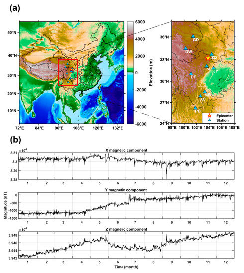
Figure 1.
The map (a) illustrates the distribution of stations (the blue triangles), and the yellow star denotes the epicenter of Jiuzhaigou earthquake. The curves (b) displays the magnetic data of the X, Y and Z components within a low-noise observation duration (i.e., 11:00 PM–05:00 AM) per day in 2017 at the Songpan (SP) station.
2. Methodology
Parkinson [26] proposed a short-term relationship among D (declination), H (horizontal) and Z (vertical) components (or X (north-south), Y (east-west) and Z components) in the geomagnetic field. Changes in these components can form a plane that is called “preferred plane” [26]. The reverse inclination of the plane reflects the direction of the high-conductivity structure, and the larger dip of the plane indicates greater difference in conductivity. The Parkinson vector [27] was proposed to indicate the inclination of the plane pointing toward the region where the conductivity is higher than nearby in the southern hemisphere. In practice, the vectors are derived from the magnetic transfer function [29]:
where Z(f), X(f) and Y(f) are the power spectrums at the particular frequency of f, while A(f) and B(f) are the coefficients of the magnetic transfer function. Each comprises the real part (Ar(f) and Br(f)) and the imaginary part (Au(f) and Bu(f)) and is written as follows:
The azimuth Pa(f) and magnitude Pm(f) of the Parkinson vectors can be calculated utilizing Ar(f) and Br(f) through the following formulas:
We computed the X(f), Y(f) and Z(f) values using a moving window of 3 hours with a step of one minute, while Ar(f) and Br(f) were calculated from every two minutes. The center of the window moves from 00:30 AM to the end of 3:30 AM. Note that f in a frequency band of 0.005–0.01 Hz is utilized for explanation in the text. In addition, f values in a relatively low frequency band (0.001–0.005 Hz) and a relatively high frequency band (0.01–0.05 Hz) were considered for an overview of the seismo-conductivity anomalies in a wide band. A total of 179 Parkinson vectors were obtained in one day.
When the Parkinson vectors are utilized to investigate the seismo-conductivity anomaly before an earthquake, the influences from the underlying inhomogeneous electrical structure around the stations have to be considered. Because locations of high conductivity materials underground can be considered to be persistent [32,38] within in one year, the background azimuth distribution was constructed by utilizing the entire Pa(f) at each station in 2017. Meanwhile, to mitigate noise and the influences of periodic variations (i.e., semi-diurnal, diurnal and semi-moon variations) on the geomagnetic data, and to have sufficient capacity of earthquake forecast in the time scale, the monitoring distributions were computed utilizing Pa(f) within a 15-day moving window (also see [32,38]) to examine the relationship between Pa(f) and earthquakes. Note that the background and monitoring distributions were binned by 10°. The count of Pa(f) in each bin is divided by the total number of Pa(f) as normalization on the background and monitoring distributions for fair comparison. The normalized background distribution was subtracted from the normalized monitoring distributions to mitigate the influence of underlying inhomogeneous electrical structures at each station. The difference obtained was further divided by the normalized background distribution in each bin to compute the anomalous proportion. The division is utilized to fairly determine the anomalous proportion in each bin. The anomalous proportions both in a particular direction and in the reverse direction are replaced by the largest value due to that the Parkinson vectors can point toward or away from the epicenters during earthquakes [38]. Finally, the anomalous proportions are further divided by the maxima of them as the normalized anomalous proportions in each day that is benefit for fair comparison among different time and distant stations. Note that those processes limit the normalized anomalous proportions ranged between 0% and 100%. A radiation map was constructed by using the normalized anomalous proportions to reveal anomaly in distinct directions referring to a station in the spatial domain. We assumed that the conductivity anomaly can dominate the Parkinson vectors that are derived from areas with distance less than 400 km (also see [29]). We superimposed these radiation maps retrieved from the stations as an integrated map to mitigate disturbances from unknown factors via formula (6),
where AVEi is the average value in the ith grid (0.1° × 0.1°) for the integrated map; Vs,i is the value of the normalized anomalous proportions in the ith grid for the s station that is located within the distance of 400 km from the ith grid; n is the total number of the stations with a distance less than 400 km from the ith grid. Note that grids in an integrated map, which are covered by at least 3 stations (i.e., n >= 3), are considered. Thus, an interaction area with the high-level anomaly is the location of the conductivity anomaly that would relate to earthquakes.
The normalized anomalous proportion of 80% is determined as the anomaly in this study. The determination suggests that the probability of presence of anomaly at each station in one day is 0.2. The 80% probability of presence of anomaly in an integrated map is 0.008 (= 0.23) due to a coverage of at least 3 stations that can be considered to be a rare event. Once the 80% probability of the presence of an anomaly in an integrated map continues for 10 days in an area, the probability of the presence of an anomaly is rather small (0.00810). We thus have the confidence to admit the anomaly.
3. Analysis Applied to the Geomagnetic Data in the Frequency Band of 0.005–0.01 Hz
We utilized the geomagnetic data retrieved from the three (i.e., JY, SP, and ZQ) stations that were closest to the epicenter of the Jiuzhaigou earthquake as an example to demonstrate the analytical processes employed in investigating the associated conductivity anomaly. Figure 2 shows the background distributions of the Parkinson vectors calculated by the entire study period of 2017 at the JY, SP and ZQ stations. The Parkinson vectors that were computed from the geomagnetic data at these stations did not direct toward an ocean due to that these stations are located far away from the sea water. Instead they directed toward high-conductivity materials around due to inhomogeneous electrical structure. At the SP station, the azimuths of the Parkinson vectors in the background are mainly distributed at approximately 85° toward the east. In contrast, the azimuths at the JY and ZQ stations are distributed at approximately 260° and 250°, respectively, toward the west. Those azimuths yielded an intersection in a region close to (104.00°E, 32.00°N) that agrees with the existence of a high-conductivity layer beneath the eastern Songpan-Ganzi block [41].
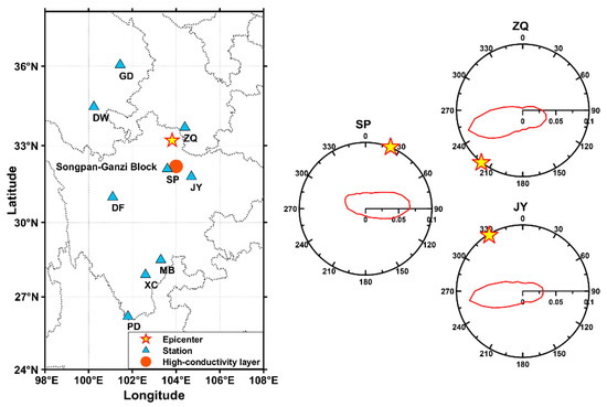
Figure 2.
The background distributions of the Parkinson vectors at the SP, ZQ and JY stations are illustrated as an example. The circle center indicates the location of each station, the radius denotes the normalized proportion of the Parkinson vectors at particular azimuths. The pentagrams show the azimuth of the epicenter relative to each station.
Figure 3 details the normalized anomalous proportions in the three selected stations from 90 days before to 15 days after the Jiuzhaigou earthquake. About 90–80 days and 60–50 days before the earthquake, the normalized anomalous proportions >80% at the SP station were respectively distributed at azimuths of about 240° and 340°, which yields a difference about 40° larger than the epicenter-to-SP azimuth and SP-to-epicenter azimuth, respectively (Figure 3a). The normalized anomalous proportions > 80% were distributed at azimuths of about 200° 40–15 days and 80–70 days before the earthquake that roughly agrees with the epicenter-to-SP azimuth (i.e., the back azimuth) (Figure 3a). About 15 days before the earthquake, the normalized anomalous proportions > 80% appeared at the azimuth of about 20° that were directed toward the epicenter of the Jiuzhaigou earthquake (Figure 3a).
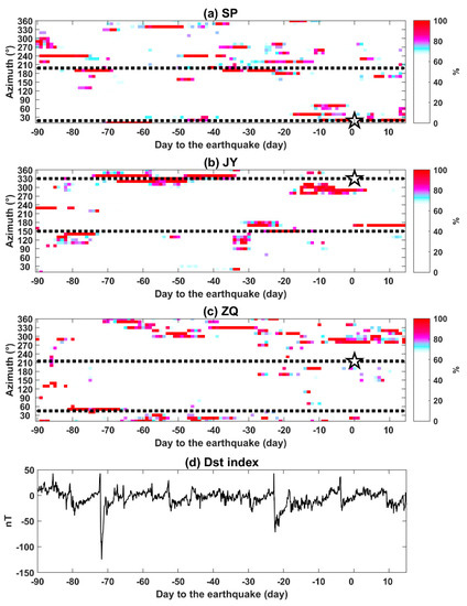
Figure 3.
The normalized anomalous proportions at the (a) SP, (b) JY, (c) ZQ stations and (d) Dst index from 90 days before to 15 days after the Jiuzhaigou earthquake. The black dash lines denote the azimuths toward either the earthquake azimuths (with the pentagram on the day of the earthquake) or the anti-earthquake azimuths. The black line in (d) shows the variations of the Dst index.
Regarding the JY station, the normalized anomalous proportions >80% were distributed at azimuths of about 150° 85–75 days and 30–20 days before the earthquake that roughly agree with the epicenter-to-JY azimuth (Figure 3b). About from 75 to 35 days before the earthquake, the normalized anomalous proportions >80% were distributed at the azimuth of about 320° to 340°, which yields within 10° related to the JY-to-epicenter azimuth (Figure 3b). About from 20 to 0 days before the earthquake, the normalized anomalous proportions >80% were distributed at the azimuth of about 300°, which yields a difference about 30° larger than the JY-to-epicenter azimuth (Figure 3b). In terms of the ZQ station, the normalized anomalous proportions > 80% were distributed at 280° and they agree with neither the ZQ-to-epicenter azimuth nor the epicenter-to-ZQ azimuth during the earthquake (Figure 3c). About 80 to 75 days before the earthquake, the normalized anomalous proportions > 80% appeared at the azimuth of about 45° that were agree with ZQ-to-epicenter azimuth (Figure 3c). An enhancement at about 10° close to the ZQ-to-epicenter azimuth appeared a few days before the earthquake (Figure 3c). Analytical results in Figure 3 suggest that the Parkinson vectors were sometimes directed toward the station-to-epicenter azimuth or the epicenter-to-station azimuth before the Jiuzhaigou earthquake. This roughly agrees with the observation in Chen et al. [37]. However, some enhancements (such as the normalized anomalous proportions > 80% at 280°–360° in Figure 3c) were caused by unknown factors that are difficult to be mitigated by using geomagnetic data retrieved from one station. If the anomaly is true, it can be observed by multiple stations, simultaneously. Thus, we constructed an integration map to eliminate unwanted influence and examine whether the anomaly can be observed by multiple stations.
The radiation maps at the three selected stations one day before the Jiuzhaigou earthquake are shown in Figure 4a–c. The epicenter was located close to the normalized anomalous proportions >80% for each station. However, the directions with the normalized anomalous proportions >80% were irrelevant to the epicenter that also existed in Figure 4a–c. If the conductivity anomaly existed, multiple stations were simultaneously able to observe it. To mitigate the unwanted influence from unknown factors and determine a location for the conductivity anomaly associated with the earthquake, these radiation maps were superimposed as an integrated map shown in Figure 4d. An intersection area that was located about 50–150 km away from the epicenter in the north was relevant to the earthquake. Meanwhile, those irrelevant directions that arose from various unknown factors were mitigated by using the integration method through considering other stations.
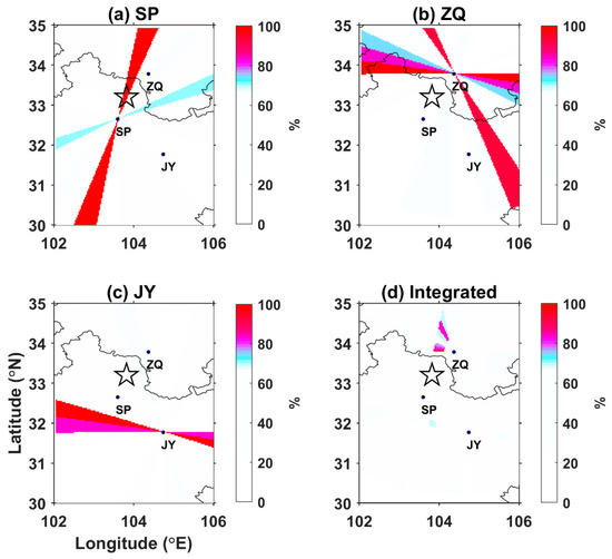
Figure 4.
The radiation maps of normalized anomalous proportions in the (a) SP, (b) JY, (c) ZQ stations, and (d) the integrated map on 7 August 2017 (one day before the earthquake). The (d) is the sum of (a), (b) and (c) divided by three. The open star represents the epicenter of the Jiuzhaigou earthquake.
We thus superimposed the entire (nine) radiation maps as an integrated map from 30 days before to 15 days after the Jiuzhaigou earthquake (Figure 5 and Figure S1). The intersections with a significant anomaly can be observed in a location (i.e., 104.00°E, 33.86°N) about 70 km away from the epicenter 17 days before the earthquake. The intersections repeat within a duration of 10 days and become insignificant 7 days before and until several days after the earthquake. Note that the probability of the presence of an anomaly is about 0.0003210 due to a coverage of 5 stations continuing for 10 days. The probability suggests that the presence of anomaly associated the Jiuzhaigou earthquake is a rare event in the time and spatial domain and cannot be usually observed in this area. Seismo-conductivity anomaly not only can be observed in the Taiwan island both also the Himalayan-China seismic regions. Note that other interactions with anomaly were also observed in the study area during the same period. However, they were generally temporary, lasting only a few days, and/or were dominated by other factors that are discussed in the following paragraphs.
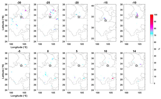
Figure 5.
The integrated seismo-conductivity anomaly maps of all nine stations at 0.005–0.01 Hz. The open star denotes the epicenter of the MW 6.5 Jiuzhaigou earthquake.
An interesting phenomenon that some sporadic anomalies start to appear far from the epicenter (i.e., 103.00°E-106.00°E, 34.00°N-36.00°N) from 30 days before the earthquake, and gradually become closer to the epicenter (Figure S1). 17 days before the earthquake, the anomalies mainly exist at the area (i.e., 104.00°E, 33.86°N) about 70 km away from the epicenter. This suggests that the stress is gradually concentrated from far distance to close the epicenter. The processes of the stress concentration roughly agree with the evolutions of crustal deformation before earthquakes observed by utilizing Global Navigation Satellite System data in Chen et al. [37,42,43]. As a result, the seismo-conductivity anomaly is a promising candidate of the pre-earthquake anomalous phenomena.
4. Discussion
We take the Dst index during the study period into account (Figure 3d). Magnetic storms occurred on 16 July 2017 (lasting for 5 days; 23-19 days before the earthquake) and 4 August 2017 (lasting for 2 days; 4–3 days before the earthquake). Meanwhile, relatively-small influence can be observed from 21 to 25 July (i.e., 18 days to 14 days before the earthquake). Although there are some magnetic disturbances from the space, the durations of those disturbances are generally limited within 1–5 days that is significantly different with the time durations (10 days for the median frequency band, 25 days for the lowest frequency band, and 12 days for the highest frequency band) of the conductivity anomaly associated with the Juizhaigou earthquake. This suggests that the conductivity anomaly reported in this study are not dominated by the disturbances from the space but probably related with the Juizhaigou earthquake.
To examine the relationships between the depths and the frequency bands proposed in Chen et al. [32], the integrated maps are constructed by using the anomalous proportions from the Parkinson vectors in the other two frequency bands (0.001–0.005 Hz in Figure 6 and Figure S2; 0.01–0.05 Hz in Figure 7 and Figure S3). The intersections with the seismo-conductivity anomaly appear around the location (105.00°E, 33.50°N) that can be observed from integrated maps using a relatively-low frequency band of 0.001–0.005 Hz from 20 days before and 5 days after the Jiuzhaigou earthquake. In addition, the anomalous intersection (105.00°E, 33.50°N) can be also observed in the integrated maps using a relatively-high frequency band of 0.01–0.05 Hz from 13 days to 1 day before the Jiuzhaigou earthquake. These suggest that the seismo-conductivity anomaly does not exist in a narrow band (i.e., 0.005–0.01 Hz) but in a wide one (i.e., 0.001–0.05 Hz) (also listed in Table 2). The seismo-conductivity anomalies are detectable by magnetometers with a sampling interval of 1 minute. On the other hand, the studied frequency bands and hypocenter depths are independent. The relationships proposed in Chen et al. [32] would be caused by earthquakes with similar depths of about 20 km in the Taiwan region.
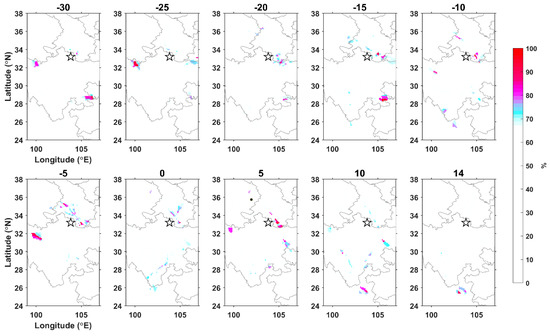
Figure 6.
The integrated seismo-conductivity anomaly maps of all nine stations at 0.001–0.005 Hz. The black star denotes the epicenter of the Jiuzhaigou earthquake.
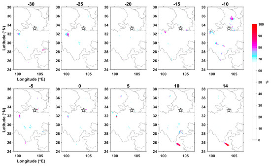
Figure 7.
The integrated seismo-conductivity anomaly maps of all nine stations at 0.01–0.05 Hz. The black star denotes the epicenter of the Jiuzhaigou earthquake.
Table 2.
The locations and time spans of the seismo-conductivity anomalies of the Jiuzhaigou earthquake obtained from different frequency bands.
Two interesting phenomena are identified from the observation of the seismo-conductivity anomaly from low to high frequency bands (Figure 5, Figure 6 and Figure 7 and Figures S1–S3). When we take the skin effect into consideration [44], a relatively-low (high) frequency reflects changes in conductivity at a relatively greater (smaller) depth. The appearance of the seismo-conductivity anomaly for the relatively low frequency band leads to its eventual occurrence in the high frequency bands (i.e., 20 days before for the lowest band, 17 days before for the median band and 13 days before for the highest band). This suggests that the seismo-conductivity anomaly associated with the Jiuzhaigou earthquake originates from a large depth and extends upwards to shallower levels. The extension agrees with the theory of seismogenic processes that stress builds in the lower crust before affecting upper curst triggering the dislocation of faults [45,46,47].
However, the disappearance and/or decrease of the seismo-conductivity anomaly a few days before the earthquake can be observed from the integrated maps among three studied frequency bands (Figure 5, Figure S1, Figure 7 and Figure S3; i.e., 7 days before for the median band and 1 day before for the highest band). This disappearance and/or decrease suggests that another physical mechanism dominates the seismogenic zone a few days before the earthquake occurs. Previous studies suggest that seismo-electromagnetic anomalies are dominated by the accumulation of earthquake-related stress in the crust [20,21,22,23,24]. In contrast, an increase of micro-cracks along faults has been observed and reported in previous studies [48,49,50,51]. The increase of micro-cracks suggests that at this time the status of the earthquake-related stress accumulation driving the variations of susceptibility and conductivity [20,21] has changed. The numbers of micro-cracks release accumulation of earthquake-related stress, and this mitigates the seismo-conductivity anomaly a few days before earthquakes. This lack of seismo-anomaly a few days before earthquakes can also be observed by using the total electron content (TEC) in the ionosphere [52]. Although upward propagation of acoustic-gravity waves [53,54] is one of the potential mechanisms of the TEC anomaly, the TEC can also be driven by the seismo-electromagnetic anomalies on the Earth’s surface [55]. Note that the seismo-conductivity anomaly can be observed from 20 days before to 5 days after the earthquake for the lowest frequency band. This would be caused by the elevated temperature of the plastic deep crust where rock is too ductile to crack [45,56]. As for the anomalies that happened at epicentral direction after the earthquake (i.e., Figure 3a), they would be caused by the stress along the fault not been fully released after the event.
Although the seismo-conductivity anomaly appears with a duration of about 10 (from 17 days to 7 days before the earthquake) days close to the epicenter of the Jiuzhaigou earthquake, other anomalies located in different places are also considered in Figure 5. The intersections with the seismo-conductivity anomaly are located around (105.50°E, 28.20°N) from 13 to 12 days before the earthquake. Note that the anomaly located around (105.50°E, 28.20°N) can also be observed from the integrated maps by using the Parkinson vectors at the relatively low frequency band from 20 to 13 days before the earthquake (Figure S2). The anomalous intersections can be referred to an earthquake (104.68°E, 28.13°N) with a small magnitude occurring on July 30, 2017 (MS = 3.0, depth = 8 km from CENC). The epicenter is about 570 km away from the Jiuzhaigou earthquake. In contrast, the intersections with the seismo-conductivity anomaly were located around (100.50°E, 31.50°N) and (104.00°E, 35.50°N) in the integrated maps by using the relatively high frequency band from 15 to 1 day and from 10 to 6 days before the earthquake, respectively (Figure S3). The anomalous intersections were also located around (100.50°E, 31.50°N) in the integrated maps by using the relatively low-frequency band from 30 to 24 days and from 7 to 4 days before the earthquake. A location around (100.50°E, 31.50°N) is related to a region in the Daofu county (101.00°E, 31.00°N) that is rich in iron ore [57], while a location at (104.00°E, 35.50°N) is caused by an unknown reason. This suggests that disturbances from high susceptibility materials underground directly affecting the geomagnetic field are difficult to remove and/or mitigate using this method. However, the disturbance is distributed within a particular frequency band that is different from the wide band that exhibits the seismo-conductivity anomaly. It can be excluded that this is due to geological characteristics.
5. Conclusions
The seismo-conductivity anomalies before the Jiuzhaigou earthquake can be simultaneously observed by the geomagnetic stations with an epicentral distance from 63 km to 385 km. The seismo-conductivity anomaly distributed in a wide frequency band of 0.001–0.05 Hz is in an area located about 70 km far from the epicenter. The anomaly appears at a deep depth and gradually extends to a shallow depth triggering the earthquake that can be obtained by using distinct frequency bands once the skin effect is considered. These anomalies are excited by the earthquake-related stress that accumulates in the crust. In contrast, their disappearance a few days before the earthquake would be dominated by an increase in micro-cracks that partially releases the accumulated stress and/or the associated frequency tends to high. These suggest that the seismo-conductivity anomaly is detectable by using far geomagnetic stations through a remote sensing analysis method. Meanwhile, these results show that seismo-electromagnetic anomalies can be integrated with multiple physical parameters to construct the potential mechanisms studying anomalous changes during seismogenic processes.
Supplementary Materials
The following are available online at https://www.mdpi.com/2072-4292/12/11/1777/s1. Figures S1–S3 shows the integrated maps of the entire (i.e., nine) stations from 30 days before and 15 days after the Jiuzhaigou earthquake at 0.005–0.01 Hz, 0.001–0.005 Hz and 0.01–0.05 Hz, respectively.
Author Contributions
Conceptualization, C.-H.C.; methodology, C.-H.C.; software, Z.M.; validation, Z.M.; formal analysis, Z.M. and C.-H.C.; investigation, Z.M.; resources, S.Z. and A.Y.; data curation, Z.M.; writing—original draft preparation, Z.M.; writing—review and editing, C.-H.C., H.Y., C.Y. and J.-Y.L.; visualization, Z.M.; supervision, C.-H.C.; project administration, C.-H.C.; funding acquisition, C.-H.C., S.Z., A.Y. and J.-Y.L. All authors have read and agreed to the published version of the manuscript.
Funding
This research was funded by National Key R&D Program of China, grant number 2018YFC1503705; Ministry of Science and Technology of the Republic of China, Taiwan, grant number MOST 107-2119-M-008-018 and MOST 108-2119-M-008-001; Sichuan earthquake Agency-Research Team of GNSS based geodetic tectonophysics and mantle-crust dynamics of Chuan-Dian region, grant number 201803; National Natural Science Foundation of China, grant number 41974073 and China Earthquake Science Foundation of Xinjiang, grant number 202001. Meanwhile, this work was also supported by the Center for Astronautical Physics and Engineering (CAPE) from the Featured Area Research Center program within the framework of Higher Education Sprout Project by the Ministry of Education (MOE) in Taiwan.
Acknowledgments
The authors appreciate the Institute of Geophysics, China Earthquake Administration provide high-quality geomagnetic data to this study.
Conflicts of Interest
The authors declare no conflict of interest.
References
- Chen, C.H.; Liu, J.Y.; Yang, W.H.; Yen, H.Y.; Hattori, K.; Lin, C.R.; Yeh, Y.H. SMART analysis of geomagnetic data observed in Taiwan. Phys. Cheam PT A,B,C 2009, 34, 350–359. [Google Scholar] [CrossRef]
- Chen, C.H.; Liu, J.Y.; Chang, T.M.; Yeh, T.K.; Wang, C.H.; Wen, S.; Yen, H.Y.; Hattori, K.; Lin, C.R.; Chen, Y.R. Azimuthal propagation of seismo-magnetic signals from large earthquakes in Taiwan. Ann. Geophys. 2012, 55, 63–71. [Google Scholar] [CrossRef]
- Chen, C.H.; Liu, J.Y.; Lin, P.Y.; Yen, H.Y.; Hattori, K.; Liang, W.T.; Chen, Y.I.; Yeh, Y.H.; Zeng, X.P. Pre-seismic geomagnetic anomaly and earthquake location. Tectonophysics 2010, 489, 240–247. [Google Scholar] [CrossRef]
- Chen, C.H.; Yeh, T.K.; Liu, J.Y.; Wang, C.H.; Wen, S.; Yen, H.Y.; Chang, S.H. Surface Deformation and Seismic Rebound: Implications and Applications. Surv. Geophys. 2011, 32, 291–313. [Google Scholar] [CrossRef]
- Fraser-Smith, A.C.; Bernardi, A.; McGill, P.; Ladd, M.E.; Helliwell, R.; Villard, O.G., Jr. Low-frequency magnetic field measurements near the epicenter of the Ms 7.1 Loma Prieta earthquake. Geophys. Res. Lett. 1990, 17, 1465–1468. [Google Scholar] [CrossRef]
- Han, P.; Hattori, K.; Hirokawa, M.; Zhuang, J.; Chen, C.H.; Febriani, F.; Yamaguchi, H.; Yoshino, C.; Liu, J.Y.; Yoshida, S. Statistical analysis of ULF seismomagnetic phenomena at Kakioka, Japan, during 2001-2010. J. Geophys. Res. Space Phys. 2014, 119, 4998–5011. [Google Scholar] [CrossRef]
- Han, P.; Hattori, K.; Huang, Q.H.; Hirano, T.; Ishiguro, Y.; Yoshino, C.; Febriani, F. Evaluation of ULF electromagnetic phenomena associated with the 2000 Izu Islands earthquake swarm by wavelet transform analysis. Nat. Haz. Earth Sys. 2011, 11, 965–970. [Google Scholar] [CrossRef]
- Han, P.; Hattori, K.; Huang, Q.H.; Hirooka, S.J.; Yoshino, C. Spatiotemporal characteristics of the geomagnetic diurnal variation anomalies prior to the 2011 Tohoku earthquake (Mw 9.0) and the possible coupling of multiple pre-earthquake phenomena. J. Asian Earth Sci. 2016, 129, 13–21. [Google Scholar] [CrossRef]
- Han, P.; Hattori, K.; Xu, G.; Ashida, R.; Chen, C.H.; Febriani, F.; Yamaguchi, H. Further investigations of geomagnetic diurnal variations associated with the 2011 off the Pacific coast of Tohoku earthquake (Mw 9.0). J. Asian Earth Sci. 2015, 114, 321–326. [Google Scholar] [CrossRef]
- Hayakawa, M.; Ito, T.; Smirnova, N. Fractal analysis of ULF geomagnetic data associated with the Guam Earthquake on August 8, 1993. Geophys. Res. Lett. 1999, 26, 2797–2800. [Google Scholar] [CrossRef]
- Hayakawa, M.; Itoh, T.; Hattori, K.; Yumoto, K. ULF electromagnetic precursors for an earthquake at Biak, Indonesia on February 17, 1996. Geophys. Res. Lett. 2000, 27, 1531–1534. [Google Scholar] [CrossRef]
- Hayakawa, M.; Kawate, R.; Molchanov, O.A.; Yumoto, K. Results of ultra-low-frequency magnetic field measurements during the Guam Earthquake of 8 August 1993. Geophys. Res. Lett. 1996, 23, 241–244. [Google Scholar] [CrossRef]
- Liu, J.Y.; Chen, C.H.; Chen, Y.I.; Yen, H.Y.; Hattori, K.; Yumoto, K. Seismo-geomagnetic anomalies and M⩾5.0 earthquakes observed in Taiwan during 1988–2001. Phys. Chem. Earth Parts A/B/C 2006, 31, 215–222. [Google Scholar] [CrossRef]
- Molchanov, O.A.; Hayakawa, M. Seismo-electromagnetics and Related Phenomena: History and Latest Results; Terrapub: Tokyo, Japan, 2008; ISBN 978-4-88704-143-1. [Google Scholar]
- Molchanov, O.A.; Kopytenko, Y.A.; Voronov, P.M.; Kopytenko, E.A.; Matiashvili, T.G.; Fraser-Smith, A.C.; Bernardi, A. Results of ULF magnetic field measurements near the epicenters of the Spitak (Ms = 6.9) and Loma Prieta (Ms = 7.1) earthquakes: Comparative analysis. Geophys. Res. Lett. 1992, 19, 1495–1498. [Google Scholar] [CrossRef]
- Tsai, Y.B.; Liu, J.Y.; Shin, T.C.; Yen, H.Y.; Chen, C.H. Multidisciplinary Earthquake Precursor Studies in Taiwan: A Review and Future Prospects; John Wiley & Sons: Hoboken, NJ, USA, 2018; pp. 41–65. ISBN 978-1-1191-5693-2. [Google Scholar]
- Wen, S.; Chen, C.H.; Yen, H.Y.; Yeh, T.K.; Liu, J.Y.; Hattori, K.; Han, P.; Wang, C.H.; Shin, T.C. Magnetic storm free ULF analysis in relation with earthquakes in Taiwan. Nat. Haz. Earth Sys. 2012, 12, 1747–1754. [Google Scholar] [CrossRef]
- Xu, G.; Han, P.; Huang, Q.H.; Hattori, K.; Febriani, F.; Yamaguchi, H. Anomalous behaviors of geomagnetic diurnal variations prior to the 2011 off the Pacific coast of Tohoku earthquake (Mw9. 0). J. Asian Earth Sci. 2013, 77, 59–65. [Google Scholar] [CrossRef]
- Telesca, L.; Lapenna, V.; Macchiato, M.; Hattori, K.J.E.; Letters, P.S. Investigating non-uniform scaling behavior in Ultra Low Frequency (ULF) earthquake-related geomagnetic signals. Earth Planet. Sc. Lett. 2008, 268, 219–224. [Google Scholar] [CrossRef]
- Nagata, T. Anisotropic magnetic susceptibility of rocks under mechanical stresses. Pure Appl. Geophys. 1970, 78, 110–122. [Google Scholar] [CrossRef]
- Stacey, F.D. Theory of the magnetic susceptibility of stressed rock. Philos. Mag. A J. Theor. Exp. Appl. Phys. 1962, 7, 551–556. [Google Scholar] [CrossRef]
- Egbert, G. On the generation of ULF magnetic variations by conductivity fluctuations in a fault zone. Pure Appl. Geophys. 2002, 159, 1205–1227. [Google Scholar] [CrossRef]
- Johnston, M.J.S. Review of electric and magnetic fields accompanying seismic and volcanic activity. Surv. Geophys. 1997, 18, 441–476. [Google Scholar] [CrossRef]
- Nishida, Y.; Sugisaki, Y.; Takahashi, K.; Utsugi, M.; Oshima, H. Tectonomagnetic study in the eastern part of Hokkaido, NE Japan: Discrepancy between observed and calculated results. Earth Planet. Space 2004, 56, 1049–1058. [Google Scholar] [CrossRef]
- Freund, F.T. Pre-earthquake signals: Underlying physical processes. J. Asian Earth Sci. 2011, 41, 383–400. [Google Scholar] [CrossRef]
- Parkinson, W.D. Directions of rapid geomagnetic fluctuations. Geophys. J. Int. 1959, 2, 1–14. [Google Scholar] [CrossRef]
- Parkinson, W.D. The influence of continents and oceans on geomagnetic variations. Geophys. J. Int. 1962, 6, 441–449. [Google Scholar] [CrossRef]
- DeLaurier, J.M.; Auld, D.R.; Law, L.K. geoelectricity. The Geomagnetic Response Across the Continental Margin off Vancouver Island. J. Geomagn. Geoelectr. 1983, 35, 517–528. [Google Scholar] [CrossRef][Green Version]
- Parkinson, W.D.; Jones, F.W. The geomagnetic coast effect. Rev. Geophys. 1979, 17, 1999–2015. [Google Scholar] [CrossRef]
- Gong, S.J.; Liu, S.Q.; Liang, M.J. Characteristics of geomagnetic Parkinson vector in Chinese mainland and their tectonic implication. Acta Seismol. Sin. 2017, 39, 47–63. [Google Scholar] [CrossRef]
- Teng, J.W.; Zhang, Z.J.; Zhang, B.M.; Yang, D.H.; Wang, Z.C.; Zhang, H. Geophy fields background of exceptional structure for deep latent mantle plume in Bohai Sea. Chin. J. Geophys. 1997, 40, 448–480. [Google Scholar] [CrossRef]
- Chen, C.H.; Hsu, H.L.; Wen, S.; Yeh, T.K.; Chang, F.Y.; Wang, C.H.; Liu, J.Y.; Sun, Y.Y.; Hattori, K.; Yen, H.Y.; et al. Evaluation of seismo-electric anomalies using magnetic data in Taiwan. Nat. Haz. Earth Sys 2013, 13, 597–604. [Google Scholar] [CrossRef]
- Gong, S.J.; Chen, H.R.; Zhang, C.F.; Yang, C.J.; Yang, C.J.; Ma, S.Q. The anomalous reactions of the geomagnetic horizontal field transfer functions before Tangshan earthquake. Acta Seismol. Sin. 1997, 10, 61–70. [Google Scholar] [CrossRef]
- Gong, S.J.; Tian, Z.L.; Qi, C.Z.; He, S.M.; Yan, X.M.; Chen, H.R. Short-term precursor of the geomagnetic horizontal field transfer functions. Acta Seismol. Sin. 2001, 14, 293–302. [Google Scholar] [CrossRef]
- Zeng, X.P.; Lin, Y.F.; Zhu, Z.J.; Xu, C.R.; Zhao, M.; Zhang, C.Y.; Liu, Q.L. Study on electric variations of media in epicentral area by geomagnetic transfer functions. Acta Seismol. Sin. 1995, 8, 413–418. [Google Scholar] [CrossRef]
- Merzer, M.; Klemperer, S.L. Modeling low-frequency magnetic-field precursors to the Loma Prieta earthquake with a precursory increase in fault-zone conductivity. Pure Appl. Geophys. 1997, 150, 217–248. [Google Scholar] [CrossRef]
- Chen, C.H.; Lin, C.H.; Wang, C.H.; Liu, J.Y.; Yeh, T.K.; Yen, H.Y.; Lin, T.W. Potential relationships between seismo-deformation and seismo-conductivity anomalies. J. Asian Earth Sci. 2015, 114, 327–337. [Google Scholar] [CrossRef]
- Chen, C.H.; Lin, C.H.; Hsu, H.L.; Wang, C.H.; Lee, L.C.; Han, P.; Wen, S.; Chen, C.S.J.T.A. Evaluating the March 27, 2013 M 6.2 Earthquake Hypocenter Using Momentary High-Conductivity Materials. Terr. Atmos. Ocean. Sci 2015, 26, 1–9. [Google Scholar] [CrossRef]
- Chen, C.H.; Tang, C.C.; Cheng, K.C.; Wang, C.H.; Wen, S.; Lin, C.H.; Wen, Y.Y.; Meng, G.; Yeh, T.K.; Jan, J.C.; et al. Groundwater-strain coupling before the 1999 Mw 7.6 Taiwan Chi-Chi earthquake. J. Hydrol. 2015, 524, 378–384. [Google Scholar] [CrossRef]
- Sun, J.B.; Yue, H.; Shen, Z.K.; Fang, L.H.; Zhan, Y.; Sun, X.Y. The 2017 Jiuzhaigou earthquake: A complicated event occurred in a young fault system. Geophys. Res. Lett. 2018, 45, 2230–2240. [Google Scholar] [CrossRef]
- Wang, X.B.; Zhang, G.; Fang, H.; Luo, W.; Zhang, W.; Zhong, Q.; Cai, X.L.; Luo, H.Z. Crust and upper mantle resistivity structure at middle section of Longmenshan, eastern Tibetan plateau. Tectonophysics 2014, 619, 143–148. [Google Scholar] [CrossRef]
- Chen, C.H.; Yeh, T.K.; Wen, S.; Meng, G.; Han, P.; Tang, C.C.; Liu, J.Y.; Wang, C.H. Unique Pre-Earthquake Deformation Patterns in the Spatial Domains from GPS in Taiwan. Remote Sens. 2020, 12, 366. [Google Scholar] [CrossRef]
- Chen, C.H.; Su, X.; Cheng, K.C.; Meng, G.; Wen, S.; Han, P.; Tang, C.C.; Liu, J.Y.; Wang, C.H. Seismo-deformation anomalies associated with the M6.1 Ludian earthquake on August 3, 2014. Remote Sens. 2020, 12, 1067. [Google Scholar] [CrossRef]
- Wheeler, H.A. Formulas for the skin effect. Proc. IRE 1942, 30, 412–424. [Google Scholar] [CrossRef]
- Hill, D.P.; Reasenberg, P.A.; Michael, A.; Arabaz, W.J.; Beroza, G.; Brumbaugh, D.; Brune, J.N.; Castro, R.; Davis, S.; dePolo, D.; et al. Seismicity remotely triggered by the magnitude 7.3 Landers, California, earthquake. Science 1993, 260, 1617–1623. [Google Scholar] [CrossRef]
- Kusznir, N.; Bott, M.H.P. Stress concentration in the upper lithosphere caused by underlying visco-elastic creep. Tectonophysics 1977, 43, 247–256. [Google Scholar] [CrossRef]
- Scholz, C.H. The Mechanics of Earthquakes and Faulting, 3rd ed.; Cambridge university press: New York, NY, USA, 2019; ISBN 978-1-316-61523-2. [Google Scholar]
- Booth, D.C.; Crampin, S.; Lovell, J.H.; Chiu, J.M. Temporal changes in shear wave splitting during an earthquake swarm in Arkansas. J. Geophys. Res. Solid Earth 1990, 95, 11151–11164. [Google Scholar] [CrossRef]
- Crampin, S.; Volti, T.; Stefánsson, R. A successfully stress-forecast earthquake. Geophys. J. Int. 1999, 138, F1–F5. [Google Scholar] [CrossRef]
- Crampin, S.C. The fracture criticality of crustal rocks. Geophys. J. Int. 1994, 118, 428–438. [Google Scholar] [CrossRef]
- Winterstein, D.; Meadows, M.A.J.G. Shear-wave polarizations and subsurface stress directions at Lost Hills field. Geophysics 1991, 56, 1331–1348. [Google Scholar] [CrossRef]
- Liu, J.Y.; Chen, Y.; Chen, C.H.; Liu, C.; Chen, C.; Nishihashi, M.; Li, J.; Xia, Y.; Oyama, K.; Hattori, K.J.J.o.G.R.S.P. Seismoionospheric GPS total electron content anomalies observed before the 12 May 2008 Mw7. 9 Wenchuan earthquake. J. Geophys. Res. Space Phys. 2009, 114. [Google Scholar] [CrossRef]
- Hayakawa, M.; Kasahara, Y.; Nakamura, T.; Muto, F.; Horie, T.; Maekawa, S.; Hobara, Y.; Rozhnoi, A.A.; Solovieva, M.; Molchanov, O.A. A statistical study on the correlation between lower ionospheric perturbations as seen by subionospheric VLF/LF propagation and earthquakes. J. Geophys. Res. Space Phys. 2010, 115. [Google Scholar] [CrossRef]
- Oyama, K.I.; Devi, M.; Ryu, K.; Chen, C.H.; Liu, J.Y.; Liu, H.; Bankov, L.; Kodama, T. Modifications of the ionosphere prior to large earthquakes-report from the Ionosphere Precursor Study Group. Geosci. Lett. 2016, 3, 6. [Google Scholar] [CrossRef]
- Liu, J.Y.; Chen, C.H.; Chen, Y.I.; Yang, W.H.; Oyama, K.I.; Kuo, K.W. A statistical study of ionospheric earthquake precursors monitored by using equatorial ionization anomaly of GPS TEC in Taiwan during 2001–2007. J. Asian Earth Sci. 2010, 39, 76–80. [Google Scholar] [CrossRef]
- Wang, S.Z. Deformation property recognition of the crust and upper mantle. Seismol. Geol. 1996, 3, 215–224. [Google Scholar]
- Luo, D.X.; Chen, Z.L.; Xiao, Y.; Xia, Z.S.; Qin, Z. Feasibility study of the development of mineral resources in Ganze Zang nationality autonomous prefecture, Sichuan province. Acta Geol. Sichuan 1993, 13, 331–356. [Google Scholar]
© 2020 by the authors. Licensee MDPI, Basel, Switzerland. This article is an open access article distributed under the terms and conditions of the Creative Commons Attribution (CC BY) license (http://creativecommons.org/licenses/by/4.0/).