Land Use Simulation of Guangzhou Based on Nighttime Light Data and Planning Policies

Abstract

With the implementation processes of strategies such as Guangdong-Hong Kong-Macau Greater Bay Area’s coordinated development and “Belt and Road Initiative” initiative, the planning policies had produced a significant influence on land use distributions in Guangzhou. In this paper, we employ nighttime light (NTL) information as a proxy indicator of gross domestic product(GDP), and a future land use simulation model (FLUS) to simulate the land use patterns in Guangzhou from 2015 to 2018 and 2018 to 2035 by incorporating planning policies. The results show that: (1) the accuracy of simulation result from 2015 to 2018 based on National Polar-orbiting Partnership, Visible Infrared Imaging Radiometer Suite (NPP/VIIRS) is higher than that based on GDP; (2) by incorporating planning policies into the model can better identify the potential spatial distribution of urban land and make the simulated results more consistent with the actual urban land development trajectory. This study demonstrates that NTL is a suitable and feasible proxy indicator of GDP for the land use simulations, providing a scientific basis for the development of urban planning and construction policy.

1. Introduction

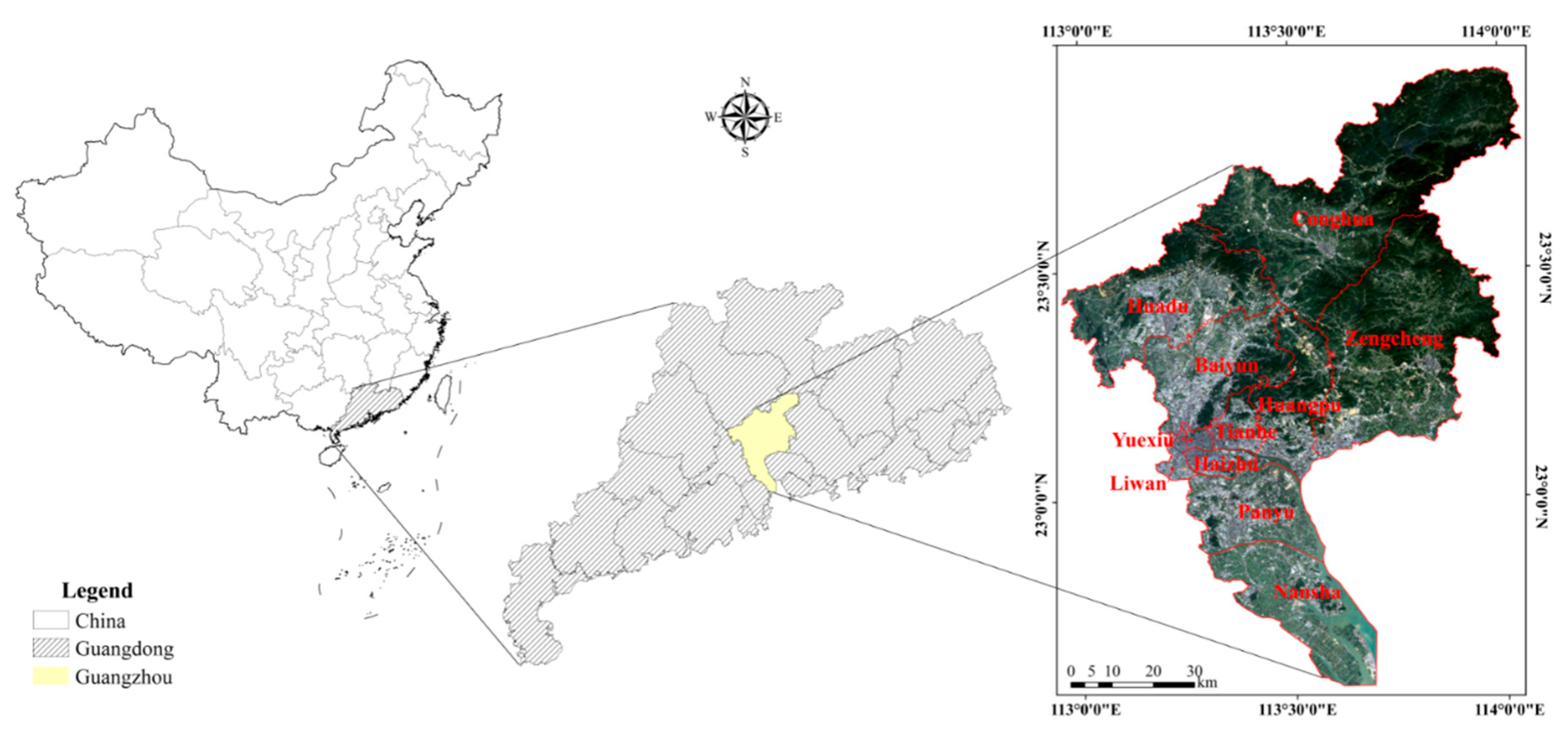
As an essential geospatial feature, land use changes play an important role in many fields, such as global ecological environmental change, urban planning, and sustainable development [1]. Since entering the industrial era, rapid urbanization has generated complex land use patterns [2]. As one of the three most economically developed cities in China, Guangzhou is a national comprehensive gateway city, the core engine of Guangdong-Hong Kong-Macau Greater Bay Area regional development, and one hub city of “Belt and Road Initiative” [3]. By 2018, the urbanization rate of Guangzhou reached 86.38%. This development has led to a variety of problems, such as excessive urban sprawl, the occupation of agricultural land, and the consequent environmental problems [4]. In the implementation processes of strategies such as Guangdong-Hong Kong-Macau Greater Bay Area’s coordinated development, the “Belt and Road” initiative, and the development pattern of “one core, one belt and one zone” in Guangdong Province, the distribution of urban land has and will continue to show a new development trend and spatial pattern. The objective and reasonable simulation of the future land use can not only grasp its changes and development laws, but also test the rationality of the current social-economic and policy-oriented land use changes. Therefore, future land use simulation by incorporating planning policies is essential for the governors when making decisions in urban land distributions and planning [5]. In 2018, Guangzhou issued the draft of “Guangzhou Land and Space Master Plan (2018–2035)” (hereinafter referred to as the GLSMP), which clearly put forward the need to constantly optimize the city landscape pattern of mountain, river, forest, built-up, rural, and sea, strictly control the intensity of urbanization, and promote conservation of intensive land. Therefore, land use simulation of Guangzhou in 2035 also has practical significance.

Recently, a large number of studies integrated topographic characteristics (e.g., digital elevation model(DEM), slope, aspect) [6], spatial location (e.g., distance to administrative center or traffic) [7], socioeconomic (e.g., population, gross domestic product(GDP)) [8] and other driving factors combined with models based on cellular theory, e.g., conversion of land use and its effects at small region extent(CLUE-S) [9,10], land transformation model(LTM) [11], agent-based model(ABM) [12], Geographical Simulation and Optimization System (GeoSOS) [13], future land use simulation (FLUS) model [8], and others for studying future land use simulation, and made significant achievement both in academic and application aspects. Through searching the existing literature, it was found that there are two problems associated with the abovementioned approach: (1) most studies used GDP as the indicator of economic development [14] or land use simulations may affect the accuracy of the results, because some GDP data might not be accurate due to inconsistent statistical scopes and institutional interference [15]. (2) land use spatial patterns are not only affected by abovementioned driving factors, but also affected by planning policies, which cannot be stereotyped and constantly changes with the urban development over time [16].

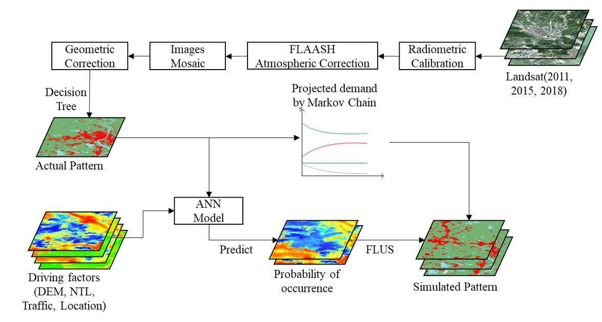
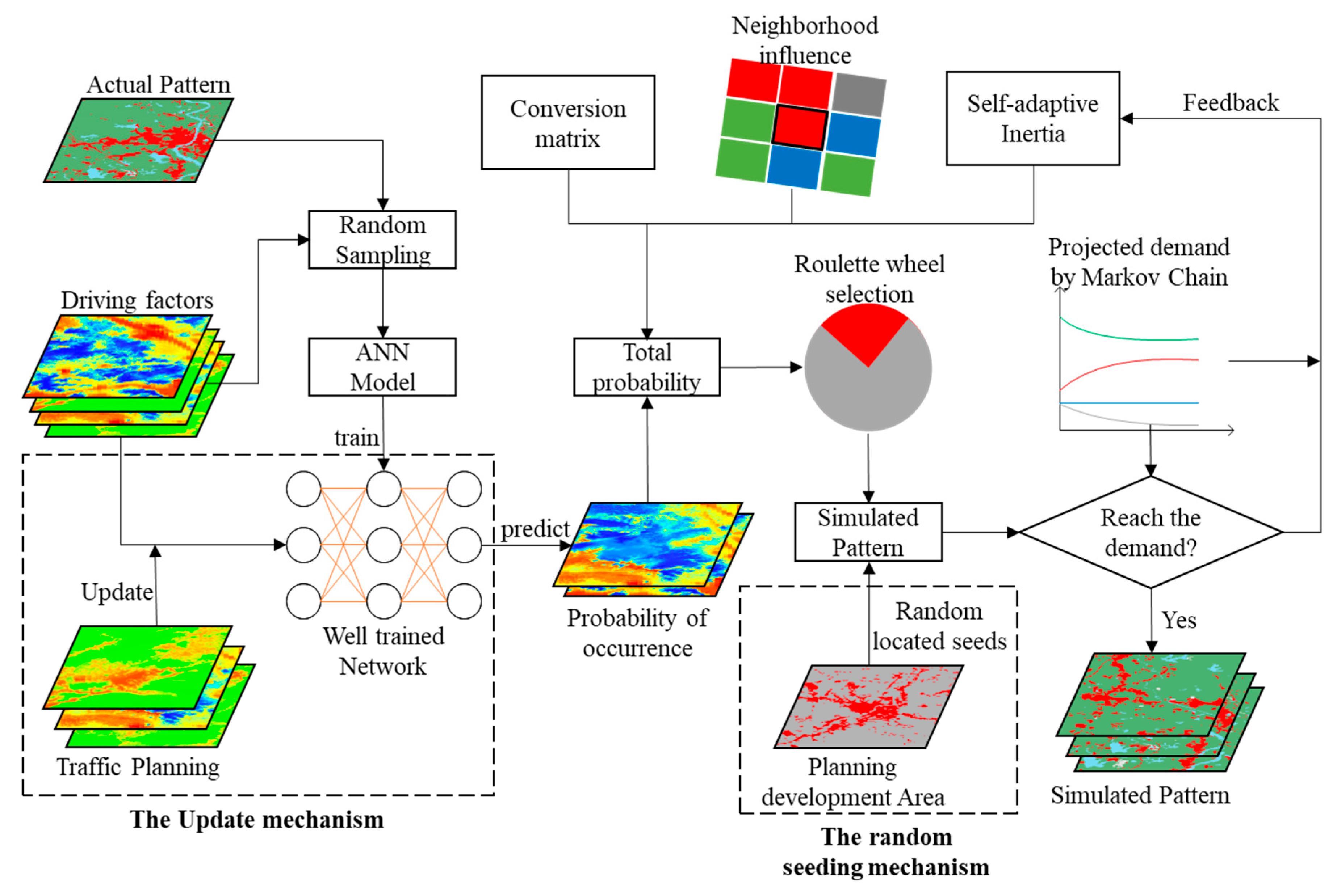
With the progress of technology, nighttime light (NTL) information has increasingly been applied to domestic and global economic studies. Compared with GDP, NTL can minimize the impact of man-made factors, and brightness of NTL may reflect the level of economic development; thus, it can serve as a proxy indicator [17]. The FLUS model (http://www.geosimulation.cn/FLUS.html) proposes two mechanisms to deal with two planning driving factors in the processes of land use simulation: (1) the artificial neural network (ANN) model for traffic planning, and (2) the random seeding algorithm for planning development zones [16].

The abovementioned problems in the currently and commonly used land use simulation methods were the reasons of initiating this study, which aims to compensate for GDP’s deficiencies by using NTL as a proxy indicator of GDP, and the FLUS model was used to address the influence of planning policies on land use distributions. Although NTL has been widely utilized for economic research [18], analyzing population/population density patterns [19], monitoring urban expansion [20], assessing ecological environment [21], building environment [22], energy consumption [23], and other fields, it has not been applied to the field of future land use simulation. At present, there are three kinds of NTL in the world: Luojia No. 1, National Polar-orbiting Partnership, Visible Infrared Imaging Radiometer Suite (NPP/VIIRS), and Defense Meteorological Satellite Program, Operational Linescan System (DMSP/OLS), with a resolution of 130 m, 500 m, and 1 km, respectively. Considering the saturation problem of DMSP/OLS, and as Luojia No. 1 has an obvious quality improvement in spatial resolution and spectral resolution than existing NTL, using Luojia No. 1, we can reflect the level of economic development more precisely. In this study, the NPP/VIIRS and Luojia No. 1 are selected to simulate the land use scenarios of Guangzhou during the period from 2015–2018 and 2018–2035, respectively.

2. Materials

2.1. Study Area

Guangzhou, the capital city of Guangdong Province, is located in (22°26′N–23°56′N, 112°57′E–114°3′E) (Figure 1), and is the “south gate” of China to the world. It covers a total area of 7277.08 km² with 11 districts, including Haizhu, Yuexiu, Liwan, Tianhe, Huangpu, Panyu, Baiyun, Huadu, Nansha, Zengcheng, and Conghua. The terrain of the study area is high in the northeast and low in the southwest, with an elevation difference of 1183 m. There are hills and mountains in the northeast, hilly basins in the middle and coastal alluvial plains in the south. As the frontier city of the reform and opening-up policy and the window of foreign trade, the economy in Guangzhou has been booming after the reform and open up policy was put forward in 1978; various undertakings have been developed into an all-round way, and Guangzhou has become one of the most active cities in China. Its comprehensive economic strength ranks among the top three cities in China. This also brings about the acceleration of urbanization, the surge of population, and the rapid expansion of urban land areas. By 2018, the resident population of Guangzhou was 14.9044 million, of which the registered population was 9.2769 million, and the urbanization rate has reached 86.38%; the GDP of Guangzhou was 22859.35 billion, which accounted for 2.56% of China’s economy; and the urban land area was 1615.00 km², which accounted for 22.19% of the study area.

2.2. Datasets and Data Processing

Land use changes are affected by a variety of driving factors. Combined with previous studies and the accessibility and accuracy of the data, historical land use patterns in 2011, 2015, and 2018 and related natural, social economic data, the development zones (e.g., traffic planning, planning development zones), and planning constraints (e.g., ecological red line, primary farmland protection, wide water bodies) are considered in the land use simulation. Prior to implementing the land use simulation model, a series of data preprocessing were carried out. Firstly, due to the radiation distortion in the process of Luojia No. 1 acquisition and transmission, the digital number(DN) value of the product is higher and resulting in a large range of bright areas, it is necessary to correct the radiation distortion of Luojia No. 1 product according to the radiation brightness conversion formula provided by the website (http://59.175.109.173:8888/app/login.html), so that the radiation distortion error can be effectively corrected and the brightness area is clearer; at the same time, some noise points are eliminated. Secondly, it is necessary to use the Euclidean Distance to preprocess the current traffic and location data, and generate the distance map to the road and administrative center. Thirdly, all datasets were converted to the same format (tiff), resolution (30 m) and projection (WGS_1984_UTM_ Zone_49N). Since all datasets used in this study, as listed in

Table 1. The data used in this study and data instruction.

Category	Data	Data Resource and Instruction
Land use	Land use data (2011, 2015, 2018)	Land use data were classified based on Landsat images, images acquisition address: https://www.usgs.gov/
Economic data	GDP	Guangzhou statistics bureau (http://tjj.gz.gov.cn/)
	NPP/VIIRS	NOAA NGDC (https://www.ngdc.noaa.gov/)
	Luojia 1	Wuhan University (http://59.175.109.173:8888/app/login.html)
Terrain	DEM	GDEMDEM (http://www.gscloud.cn/)
	Slope	Calculated from DEM
	Aspect
All levels of roads	Highway	BIGEMAP (http://www.bigemap.com/)
	Main road
	Railway
	Subway
Location	City center	BIGEMAP (http://www.bigemap.com/)
	District centers
	Town centers
Planning data	Traffic planning in Greater Bay area	Draft of “Guangzhou Land and Space Master Plan (2018-2035)
	Economic settlement zone planning
	Advanced manufacturing industry planning
	Primary farmland
	Ecological red line
	Wide water bodies	Image interpretation

, have different units and dimensions, they were all normalized to the range of [0, 1].

3. Methods

There three steps involve in the land use simulation of Guangzhou in 2035: (1) extraction of land use types from Landsat images, (2) prediction of land use demand using the Markov Chain, and (3) for spatial allocation of future land use using the FLUS model. The flowchart of methods developed in this study is illustrated in Figure 2.

3.1. Extraction of Land Use Types

Prior to applying Landsat TM/ETM+/OLI images in 2011, 2015, and 2018 (122/43, 122/44, six scenes) with a resolution of 30 m downloaded from the USGS Explorer website for classifying land use types, a series of image preprocessing were carried out including radiometric correction, fast line-of-sight atmospheric analysis of spectral hypercubes (FLAASH) atmospheric correction, band combination, image mosaic, and subset. Three land use types, i.e., urban land, non-urban, and water, were classified based on these Landsat images using the decision tree and visual interpretation method. Confusion matrix was chosen to measure the accuracy of the classified images according to the number of samples were randomly selected from Google Earth images.

3.2. Markov Chain Model

Markov chain is a random process that projecting future land use demands by generates probability of transformation matrix from one land use class to another for a specified time period [24]. First, the initial state matrix F₀ is determined; then, the probability of transformation matrix P_ab from one state a to another state b is calculated according to Equation (1):

$$P_{ab}=\frac{S_{ab}}{S_a}\times \frac{1}{n}$$

(1)

where S_ab represents the area of land transferred from state a to state b in the last year, and S_a represents the area in state a in the initial year. According to the transition probability, probability of transformation matrix P can be calculated as follows:

$$P=\left[\begin{array}{c}{P}_{11}\\ P_{21}\\ \dots \\ P_{a1}\end{array}\begin{array}{c}{P}_{12}\\ P_{22}\\ \dots \\ P_{a2}\end{array}\begin{array}{c}\dots \\ \dots \\ \dots \\ \dots \end{array}\begin{array}{c}{P}_{1b}\\ P_{2b}\\ \dots \\ P_{ab}\end{array}\right]$$

(2)

Land use changes is predicted according to Equation (3):

$$S_{\left(t+1\right)}=P_{ij}\times S_{\left(t\right)}$$

(3)

where S_(t) and S_(t+1) are the states at time t and t + 1, respectively; P_ij is probability of transformation matrix and satisfies: 0 ≤ P_ij < 1 and ${\displaystyle \sum }_{j=1}^n{P}_{ij}=1$(i, j = 0, 1, 2, … n).

3.3. FLUS Model

A CA-based FLUS model is established by coupling the ANN algorithm and the roulette wheel selection mechanism [8]. The principle of FLUS is as follows: firstly, the updated mechanism based on an ANN is used to calculate suitability probability for land use types of each cell, that is, generate the probability of occurrence for land use types on each cell. Then, the self-adaptive inertia and competition mechanism based on roulette wheel selection is used to tackle the competition between land use types in each grid. Finally, the combined probability is calculated by coupling random seeding mechanism, and the combined probability is used to deduce land use distributions under the constraints of a certain number of structures in the future. In the process of land use spatial allocation, users are required to preset simulation parameters such as development area, constraint area, land use demand, cost matrix representing the difficulty of transforming current features into target features, weight of neighborhood, the number of iterations, neighborhood size and so on. The process of simulation and model parameters are detailed in [8,16].

The schematic framework of land use simulation of the FLUS model is shown in Figure 3.

4. Results and Discussions

In this study, we divided the scenario simulation into two periods: 2015–2018 and 2018–2035. During the period from 2015–2018, 20% of the total pixels were randomly selected from the land use data in 2015, and 11 driving factors (with the exception of planning data) were used as the training dataset to train the ANN model for the probability of occurrence for land use types. The future land use distribution results were simulated by combining land demand, neighborhood influence factors, and inertia coefficients representing previous land types and conversion costs. The validity of NPP/VIIRS serve as the proxy indicator of GDP and the verification of land use patterns simulation in 2035 were assessed. However, the influence of planning policies on the accuracy of simulation cannot be validated at this stage, because traffic planning in the Greater Bay area, advance manufacturing industry planning, and economic settlement zone planning were delineated by the GLSMP in 2018. Thus, the effect of planning policies on land use distributions was only analyzed in the period from 2018–2035, in the simulation model, we used primary farmland, ecological red line, and wide water bodies as planning constrains; traffic planning in the Greater Bay area, advance manufacturing industry planning, and economic settlement zone planning were used as the development zones for future land use simulation. Nevertheless, it is generally believed that the setting of planning policies can improve the accuracy of simulation because they have a significant effect on urbanization construction; for example, the implementation of a series of policies such as ecological red line and primary farmland protection, which limits the occupation of cultivated land and forest by urban land expansion. On the contrary, the development zones mark the areas that were not originally used for urban land that have developed into urban land.

4.1. Analysis on Land Use Types Extraction

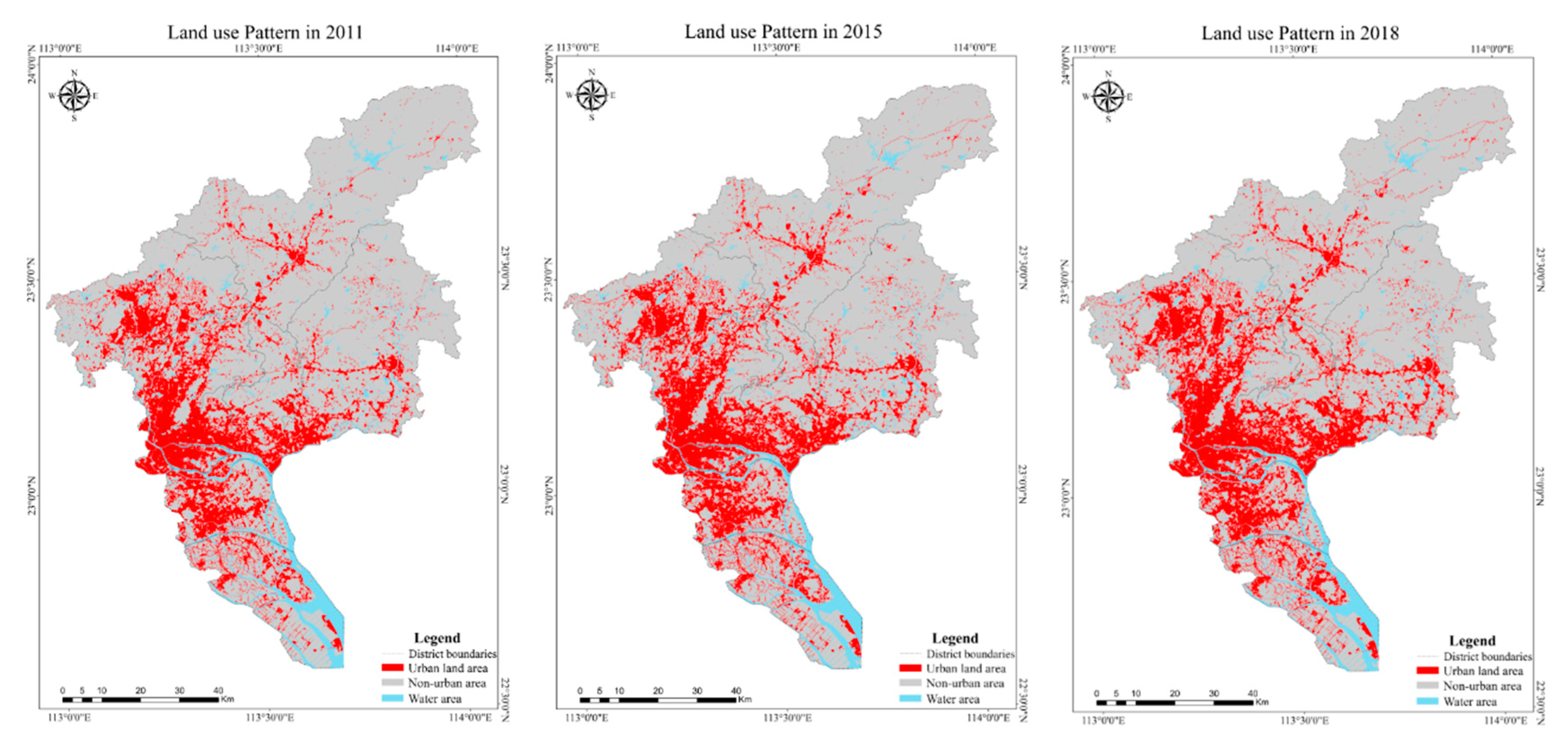
Accuracy analysis is an indispensable part of land use types extraction as it can determine whether the accuracy of the data meets the requirements. Results showed that 94.21%, 92.80%, and 92.28% of the classified images in 2011, 2015, and 2018 are consistent with Google Earth images, respectively, which meet the accuracy requirements of land use types extraction.

Figure 4 shows spatial distributions of land use types for the study area in 2011, 2015, and 2018. Generally speaking, the change trend of land use types in Guangzhou from 2011 to 2018 is that the water area has not significantly changed, the non-urban area is decreasing, and the urban land is increasing noticeably.

Combined with the analysis of the district boundary, natural environment, and planning policies, we have found that: (1) regarding traffic conditions and other factors, Zengcheng and Huangpu have the largest area of urban land expansion, namely 41.04 km² and 37.08 km², respectively. This is because under the guidance of policies, such as the construction of national economic and technological development zones and the industrial gathering area of overseas Chinese businessmen, the planning and implementation of G45 national expressway, and the urbanization of Luogang new industrial zone, the none-urban areas in and along the existing urban areas have developed into urban land. (2) Under the influence of the development of modern intermodal logistics centers, industrial clusters, university towns, free trade zones, and the improvement of urban transportation systems, urban land areas of Baiyun, Conghua, Huadu, Panyu and Nansha have expanded, namely 25.96 km², 21.82 km², 26.28 km²,20.54 km², and 24.28 km², respectively. (3) Due to the special geographical location and natural conditions of Zengcheng and Conghua, their urbanization level is relatively low. (4) Haizhu, Yuexiu, Liwan, and Tianhe belong to the old urban area of Guangzhou, and there is no space for expansion within the administrative boundary.

From the perspective of the direction of expansion, there is more urban land expansion in the south, west, and northeast. Guangzhou breaks through the traditional urban area, and extends to Panyu, Nansha, Zengcheng, Conghua, and Huadu. It can be seen that planning policies and transportation are closely related to the evolution of the spatial pattern of Guangzhou, and the overall development of cities conforms to the layout of urban master plan; the higher the connectivity of traffic, the greater the driving effect on urban development.

4.2. Land Use Simulation from 2015 to 2018

4.2.1. Prediction of Urban Probability of Occurrence Based on ANN

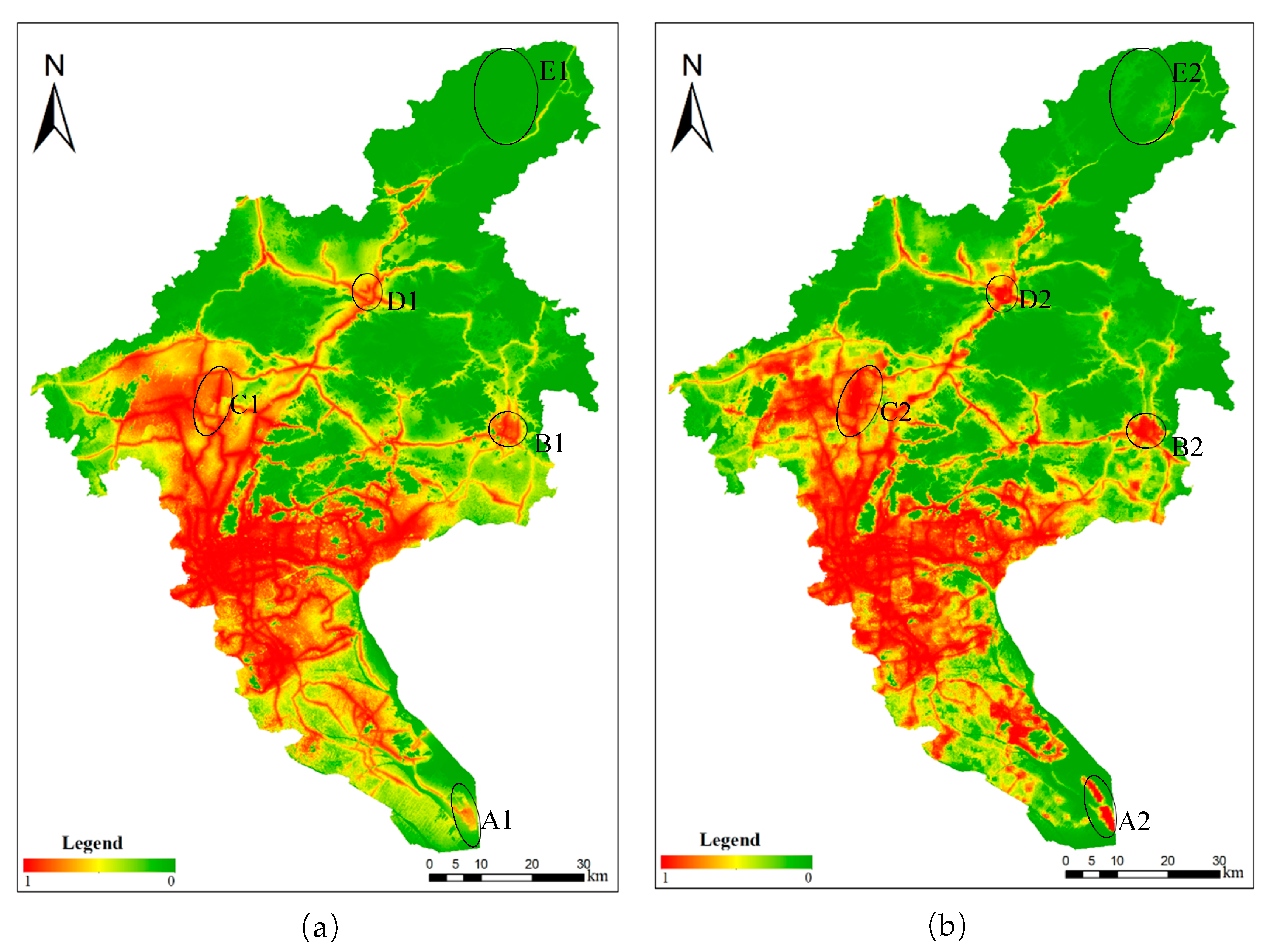
In this study, we added GDP and NPP/VIIRS separately to the ANN predicted process to analyze the influence of these two economic factors on urban land probability-of-occurrence, the generated urban land probability of occurrence surfaces are shown in Figure 5. Under the impact of different economic factors, urban land probability of occurrence shows obvious differences in spatial terms. For example, urban land probability of occurrence in the areas such as A2, B2, C2, D2, and E2 is obviously higher than that in A1, B1, C1, D1, and E1. Compared with Google Earth images, by 2018, the areas of A2, B2, C2, D2, and E2 are Guangzhou Nansha bonded Port, Zengcheng District, Guangzhou Baiyun International Airport, Conghua District, and sporadic rural settlements, all of which are urban land with high light brightness value; therefore, urban land probability of occurrence based on NPP/VIIRS is higher than that based on GDP data. These differences will affect the spatial allocation of urban land in the future.

4.2.2. Land Use Simulation Based on Probability of Occurrence

Based on urban land probability of occurrence, this study simulated urban land growth from 2015 to 2018 under the impact of two economic driving factors. During the simulation process, actual land use areas in 2018 were considered as land use demand. Finally, the real land use patterns in 2018 were employed to validate the simulation results.

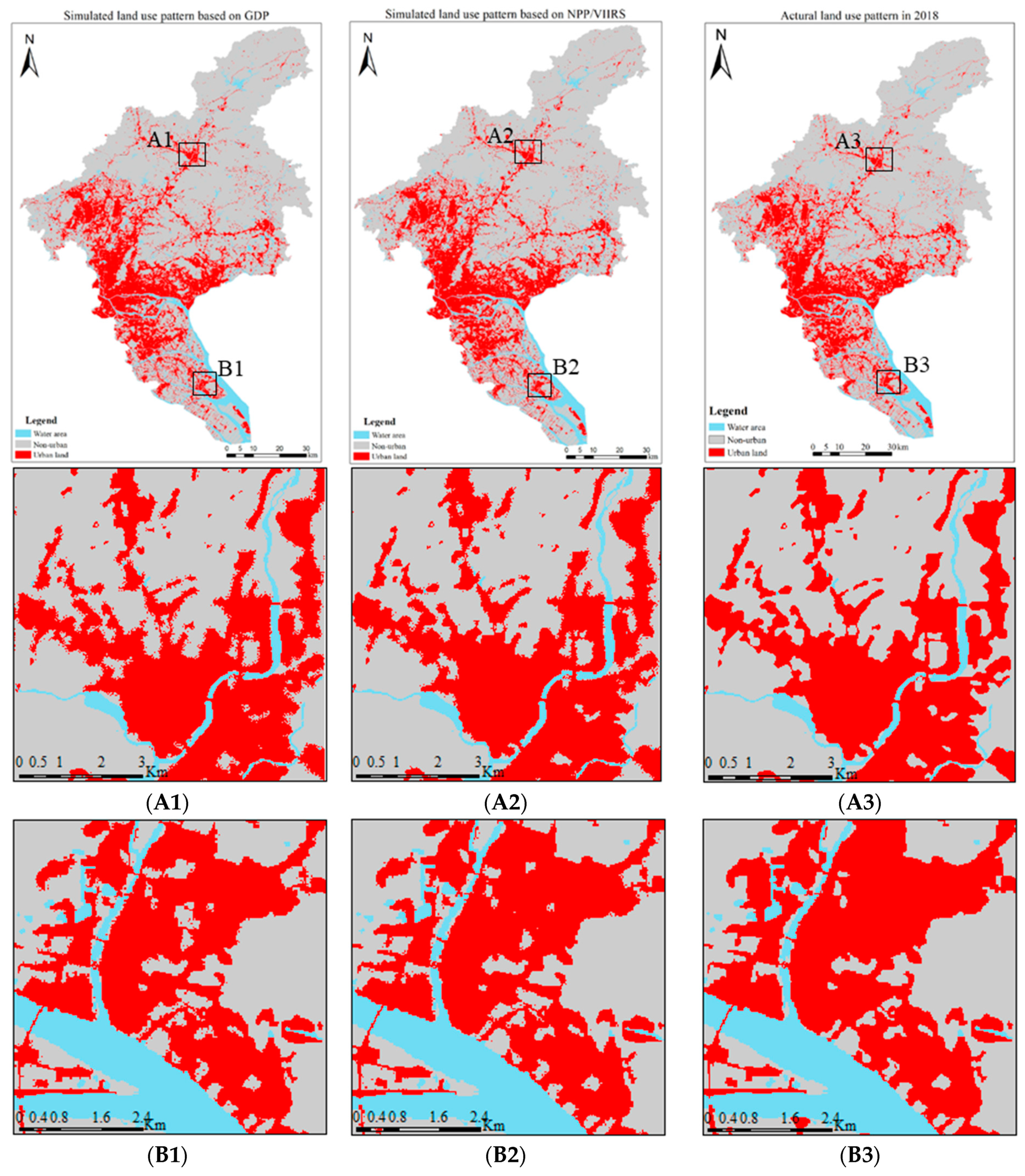
The simulated land use patterns under the impact of different economic factors and the actual land use patterns in 2018 are shown in Figure 6, and two local areas are enlarged to display more details. Figure 6 shows that the overall distribution characteristics of the simulated results are similar and similar to the actual land use patterns, but simulation accuracies are different. From the enlarged views, it can be found that the simulated patterns using NPP/VIIRS as a proxy indicator of GDP is close to the real land use patterns in 2018. However, urban land probability of occurrence in some areas is very high, and it is urban land in the real land use patterns, but the simulation result is still non-urban land. This is related to the joint probability that affects the result of land use change, which is composed of probability of occurrence, inertia coefficient, neighborhood influence, and conversion cost; the roulette wheel selection mechanism transforms the initial land use type of each cell into a land use type with higher joint probability. Further analysis shows that the range of urban land in the simulation results is larger than that in actual land use patterns, and is distributed in small patches; this is because the land use change simulation is based on the cell grid, and the NPP/VIIRS data also have a certain degree of brightness overflow.

4.2.3. Validation and Analysis of Simulation Accuracy

In order to quantitatively assess the simulated results, the figure of merit (FoM) is used to validate the agreement of the changes, which is better than the Kappa coefficient [25,26] in evaluating the change information of simulated results [27]. Theoretically, the higher the FoM, the higher the simulation accuracy, but FoM values range from 1% to 59%, and it has been proved that most of the values are less than 30% [27].

For the accuracy assessment results, although the FoM values under the influence of two economic driving factors are not highly accurate, in which the FoM value of simulated results based on GDP and NPP/VIIRS are 6.48% and 7.33%, respectively, they are acceptable for the following reasons: (1) they are close to the results in other studies. For example, the FoM value was 12.46% for land use simulation of the Pearl River Delta region in 2000 to 2010 by Liu et al. [8]. Although the FoM values in this study are less than 12.46%, according to the positive relationship between the observed net change and FoM in the study by Estoque and Murayama [28], the FoM value of a shore period simulation results is likely lower than one with a long period, given the simulation period of this study (2015–2018) is shorter than that of Liu et al. (2) The FoM of low resolution simulation is likely higher than one with high resolution. Liu et al. simulated the national land use patterns with the same period and driving factors but different resolutions (1 km × 1 km), resulting in an FoM value of 19.62%, which was higher than that of the Pearl River Delta regional land use pattern with a resolution of 250 × 250 m. Similarly, since the resolution of this study is lower than that of Liu et al., the FoM value is lower compared to the study by Liu et al. Therefore, it is feasible to use NTL as a proxy variable of GDP to measure economic development, and on this basis, we can simulate and predict the future land use distributions in Guangzhou.

4.3. Land Use Simulation from 2018 to 2035

4.3.1. The Projected Land Use Demand

In the process of land use simulation, the land demand was first determined. Then, land use distributions were deduced under the constraints of the quantification of urban land use structure; therefore, before future land use simulation, the land use demand was first projected by the Markov Chain model. At the beginning, the land use demand in 2025 was projected based on the analysis of actual land use patterns during 2011–2018. Then, actual land use patterns in 2015 and simulated land use patterns in 2025 were inputted into the Markov Chain model to project the land use demand in 2035. According to the changes of water area in the past, it can be considered that the probability of its change in the forecast period is very small; thus, it is assumed that the water area will not change in the future. The future land use demands are show in

Table 2. Future land use demands.

Year	Urban Land/km2	Non-Urban/km2	Water/km2
2025	1803.45	5002.52	471.11
2035	2069.33	4736.64	471.11

. With rapid urbanization, urban land expansion has occurred more quickly. By 2025, urban land will increase to 1803.45 km², and 2069.33 km² by 2035, corresponding to an increase of 198.43 km² and 454.31 km², respectively, compared with 2018.

4.3.2. Spatial Allocation and Analysis

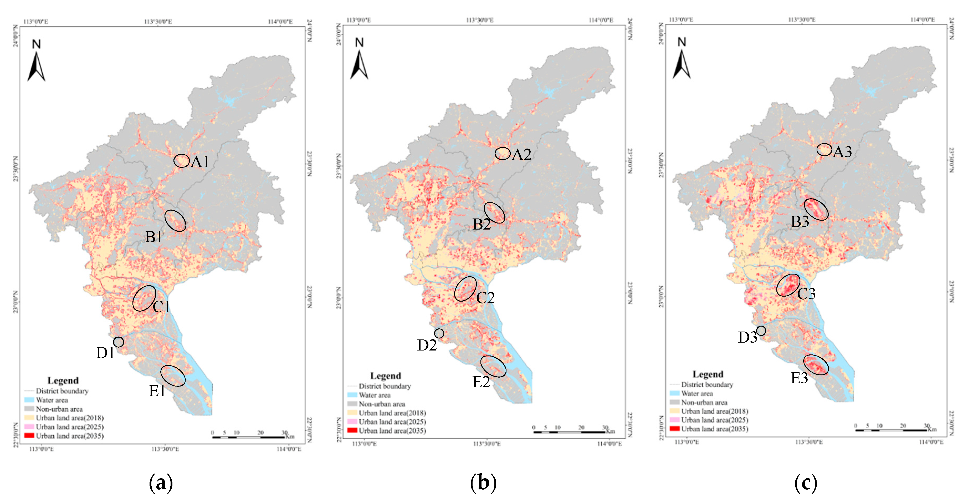
Based on the abovementioned land use demand, through the FLUS model, Luojia No. 1 was used as a proxy indicator of GDP to realize the land use scenario simulation from 2018 to 2035. Three scenarios were tested. Scenario I without any planning policies, scenario II under the influence of planning constraints, and scenario III under the influence of planning constraints areas and planning drivers. The other ten driving factors are the same as the validation simulation during the period of 2015–2018. In the scenario I, land use simulation in 2035 was predicted based on the land use changes during 2011–2018, and land use changes was not affected by planning policies adjustment. Scenario II considered only the ecological red line, the primary farmland protection areas, and wide water bodies as the planning constraints area, which cannot be used for urban land expansion. Scenario III was a comprehensive consideration of the mutual benefits between the economy development and the ecological environment; it considered not only the abovementioned planning constraints areas but also the traffic planning and planning development zones. With the exception of planning restrictions area, other areas can be used for urbanization, and there will be a greater chance for the areas of planning drivers. The simulated results in 2025 and 2035 are shown in Figure 7.

According to urban land demand, the comparison between scenario I, II, and III indicates that under the comprehensive action of driving factors, there are both similarities and differences in the spatial distribution of land use types. The same is that most land use types have expanded and contracted in and around their original location over time, in which urban land mainly spreads along the original urban land or traffic routes, while under the influence of urban development, non-urban land area is reduced obviously. The difference is that the spatial patterns of urban land expansion is different between three scenarios; promotion of planning policies significantly changes the future land use patterns and development trajectory, improves the intensity of urban land, and makes the urban form more compact. In scenario I, urban land expansion in a disorderly manner, which causes more urgent encroachment and encirclement on non-urban areas such as cultivated land, forest land, and water body (Figure 7a (A1 and D1)). This extensive land use method can easily cause adverse effects on the ecological environment. Scenario II strictly controls the occurrence of new urban land in the area through the delimitation of planning constraints areas (Figure 7b (A2 and D2)) to form centralized food production areas and ecological protected areas. Scenario III adds traffic planning and planning development zones on the basis of II, which not only ensures the bottom line of food security and ecological security, but also suppresses the phenomenon that the non-urban areas in and around the original urban areas are more likely developed into urban land, and makes the urban land develop to lumps; moreover, it causes some regions to develop urban land even with low probability or without nearby urban pixels (Figure 7c (B3, C3, and E3)). Thus, the city gradually shifts to a healthy development model. In the early stage (2018–2025), there were insignificant differences in the process of urbanization between three scenarios, but this became obvious in the later stage (2025–2035).

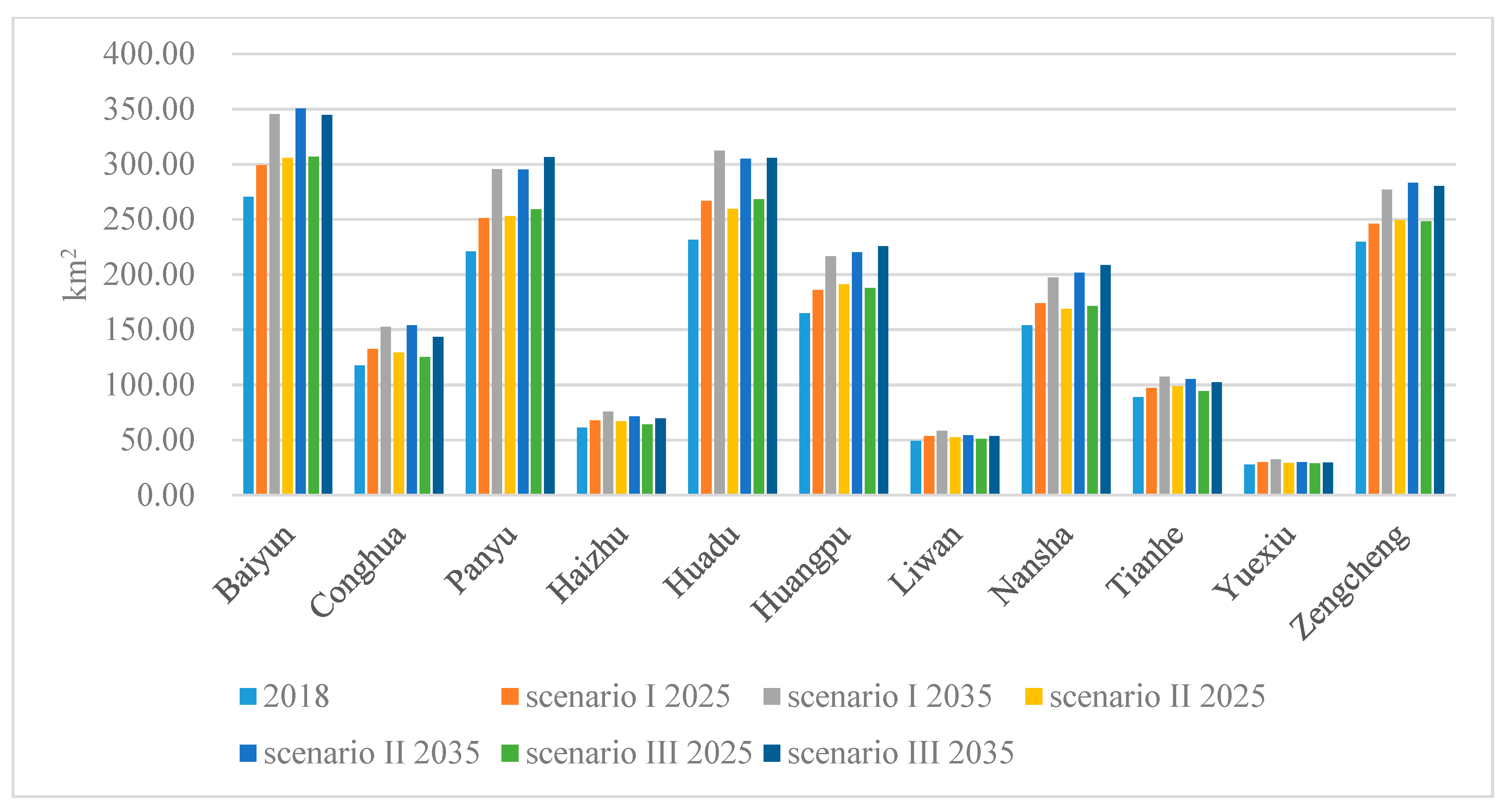
In addition, through the statistics of urban land expansion area in different districts (Figure 8), it is found that the urban land area changes differently between three scenarios. The areas that are greatly affected by government planning policies, such as Zengcheng, Huady, Baiyun, Panyu, Nansha Deputy Center, and Huangpu, have increased significantly, and will become “hot spots” for urban land expansion in the next 17 years, which is not only in accordance with the development strategy of Guangzhou, but also in accordance with the effect of the current social and economic background on the law of future land use development.

Therefore, according to the abovementioned simulation results of land use spatio-temporal changes, we should pay more attention to the land use changes in hot spots, strictly control the unreasonable transfer of land use types, and ensure to develop a sustainable urban ecological environment.

4.3.3. Evaluating the Simulated Results with the Planning Policy

In this section, the simulated results are compared with the planning policies determined in the GLSMP to assess the constraint and guiding effect of planning policies on future land use spatial patterns.

Table 3. The comparison between the simulated results and the planning policies under three scenarios.

Master Plan		2018	Scenario I		Scenario II		Scenario III
Category	Area		2025	2035	2025	2035	2025	2035
planning constrains	2373.65	0.00	40.39	99.16	0.00	0.00	0.00	0.00	urban land area
development zones	471.36	252.06	281.05	323.98	291.00	345.28	350.59	430.00
planning constrains	--	--	40.39	99.16	0.00	0.00	0.00	0.00	area of urban land expansion
development zones	--	--	28.99	71.91	38.94	93.22	98.53	177.94

shows a comparison between the simulated results and the planning policies between three scenarios.

There is no growth of urban land in the planning constraints areas between scenario II and scenario III; this is because China implements a series of strict ecological protection policies to protect the area of ecological land, such as cultivated land, water area, and forests. Compared with scenario I, because there are no policy restrictions, some high-quality agricultural lands are developed into urban land. The urban land distributions in the area of traffic planning and planning development zones in scenario III is different from that in scenario I and scenario II, because planning policies increases the proportion of urban land area on the basis of maintaining the existing quantity and layout of urban land. Generally speaking, the simulation results of land use patterns in planning year under the impact of planning constraints and planning drivers more consistent with the master plan in the GLSMP, this can more reasonably simulate land use patterns than those without any planning policies. However, some regions inside the development zones cannot develop into urban land, even if random seeding mechanism helps increase urban land probability of occurrence, because the urban land probability of occurrence in this region remains too low. However, these regions, which have not developed into urban land within the development zones, can provide data reference for the government and relevant departments to revise the GLSMP in the future, so as to make the city’s layout and planning more reasonable, achieve the dual goals of urban construction and ecological protection, and promote the city to achieve sustainable development.

In summary, the simulated results under the influence of planning policies from 2018–2035 take into account the objective laws of land use changes, planning constraints, and the development zones, which can meet the land use demand of industrial structure adjustment and urbanization on the basis of fully ensuring food security and ecological environment.

5. Conclusions

This study used the NTL information as a proxy indicator of GDP and incorporated with the FLUS model to simulate future land use patterns under the influence of planning policies. The simulated results of land use patterns under the impact of different economic driving factors show that the simulations based on NPP/VIIRS have higher accuracy, which demonstrates that the NTL is a suitable and feasible proxy indicator of GDP.

The future land use scenario simulations under the influence of planning policies showed that more urban land growth occurred in Nansha Deputy Center, Panyu, Huangpu, Zengcheng, and other districts from 2018 to 2035. This is in accordance with the development strategy of Guangzhou to optimize the formation of “one main, one deputy multi-district” economic function agglomeration area and focus on the construction of three major industrial agglomeration belts. At the same time, the simulated results also took into account the objective laws of land use changes and planning constraints; thus, the simulated results, with the introduction of planning factors, are more consistent with the real urban development trajectory and can help achieve sustainable development. In summary, the simulations presented in this study provide some useful information for urban planning.

The driving factors often change with time with adding some new characteristics, such as the continuous development of factors, including planning policies, economic development, and other factors, and will produce different impact on the land use patterns. However, this study considered the driving factors as static variables. Therefore, future studies are necessary to include the temporal variations of the driving factors in the land use simulations, and focus on the interactions between driving factors and land use changes. In addition, research by Lawler et al. [29] showed that differences in the underlying drivers of land use change, such as changes in future crop prices, can have large impacts on land use simulations, which will change as a response to the land use policies. Thus, how to predict the land use change in terms of coupling the spatial analysis approach with endogenous price feedbacks from land use policies can be left for further research.