Abstract
Remote sensing, particularly using synthetic aperture radar (SAR) systems, can be an effective tool in detecting and assessing the area and amount of building damages caused by earthquake or tsunami. Several studies have provided experimental evidence for the importance of polarimetric SAR observations in building damage detection and assessment, particularly caused by a tsunami. This study aims to evaluate the practical applicability of the polarimetric SAR observations to building damage caused by the direct ground-shaking of an earthquake. The urban areas heavily damaged by the 2016 Kumamoto earthquake in Japan have been investigated by using the polarimetric PALSAR-2 data acquired in pre- and post-earthquake conditions. Several polarimetric change detection approaches, such as the changes of polarimetric scattering powers, the matrix dissimilarity measures, and changes of the radar scattering mechanisms, were examined. Optimal damage indicators in the presence of significant natural changes, and a novel change detection method by the fuzzy-based fusion of polarimetric damage indicators are proposed. The accuracy analysis results show that the proposed automatic classification method can successfully detect the selected damaged areas with a detection rate of 90.9% and false-alarm rate of 1.3%.
1. Introduction
Earthquakes are one of the major natural disasters. The direct ground-shaking and secondary effects, e.g., tsunami, can cause numerous structural failures in urban areas, resulting in human fatalities. After earthquake or tsunami disasters, it is important to quickly ascertain the area and amount of building damage. Remote sensing, using satellite images, can be an effective tool in monitoring damage over a wide area. Particularly for rapid damage detection, synthetic aperture radar (SAR) systems can provide timely and reliable data suitable for monitoring disasters.
The SAR-based detection of building damages caused by earthquake and tsunami has been studied mainly by the change detection method using single-polarization multitemporal SAR images acquired at pre- and post-disaster conditions. Matsuoka and Yamazaki [1] analyzed changes in the backscattering coefficients and intensity correlation using ERS SAR data for detecting building damages caused by the 1995 Kobe earthquake. By combining the two parameters, the damage discriminant index was proposed to highlight building-damaged areas. It was further refined and applied to the 2003 Bam earthquake [2], the 2004 Niigata earthquake [3], and the 2016 Kumamoto earthquake [4]. The damage indices derived from the intensity difference and the intensity correlation agreed well with the in situ data but showed significant variances in both target and background areas. An improvement of the damage augmentation was proposed in [5] by using additional pre-seismic intensity correlation in the change detection. The difference between the co-seismic and pre-seismic intensity correlations corresponded well to the collapse ration in the case of the 2003 Bam earthquake. In [6], the sensitivities of the normalized intensity difference and the intensity correlation to damage grades were evaluated using the high-resolution TerraSAR-X and Cosmo-SkyMed data. The experiments for the 2010 Haiti earthquake showed that the normalized intensity difference provided better correlation with damage grades. It was also pointed out that the sensitivity of SAR parameters to damage grades can be significantly affected by the temporal baseline between the pre-and post-earthquake acquisitions.
In order to improve the detectability of building damages, several recent studies focused on the use of polarimetric scattering information. Park et al. [7] analyzed various polarimetric parameters of ALOS PALSAR data and proposed an unsupervised detection method for tsunami-flooded areas and swept urban areas caused by the 2011 Tohoku earthquake. The experimental results showed that the polarimetric depolarization indicators such as the polarimetric coherence and the entropy provided significant improvement of detection accuracy as compared with the single-polarization intensity. In the case of mapping swept urban areas, the polarimetric similarity parameter provided the best detection performance, with an overall accuracy of about 89%. For the same Tohoku earthquake, Chen and Sato [8], and Chen et al. [9] studied the possibility of estimating the level of building damages caused by tsunami using the multitemporal PALSAR data. Changes in the polarimetric double-bounce scattering power were found to be an effective index to indicate the damage level.
Previous studies have provided experimental evidence for the importance of polarimetric SAR observations in building-damage detection and assessment. However, these studies were conducted on tsunami damages, which are relatively infrequent, and the damage patterns may differ from the building damages caused by typical land earthquakes. This study aims to evaluate the practical applicability of the polarimetric SAR observations to building damages caused by direct ground-shaking. In this study, various polarimetric change detection approaches are examined, and an effective detection method for mapping the building damaged areas is proposed. The heavily damaged urban areas by the 2016 Kumamoto earthquake in Japan were investigated by using the polarimetric PALSAR-2 data acquired in pre- and post-earthquake conditions. This paper is organized as follows. In Section 2, the study area and a description of the acquired SAR data used for this paper are discussed. Different polarimetric change detection methods are examined in Section 3. The unsupervised detection method to classify building-damaged areas and the accuracy analysis results are presented in Section 4. Discussion on the detection results in relation to the previous studies and the survey data are given in Section 5, and summaries and concluding remarks are presented in Section 6.
2. Study Area and Data Set
The study site is the Mashiki town in the Kumamoto area (white rectangle in Figure 1). This area was among the most seriously affected by a series of earthquakes that occurred in Kumamoto, Kyushu Island, Japan on 14 April (foreshock, Mw 6.2.) and April 16 (mainshock, Mw 7.0.), 2016. The intense seismicity of the earthquakes was distributed along the active Futagawa fault (red dashed line in Figure 1a) running through the study site [10]. The field survey reported that more than 7000 buildings in this area were severely damaged due to intensive ground-shakings [11]. In order to detect the damaged buildings by the earthquakes, two temporal PALSAR-2 data sets, obtained five days after (21 April 2016) the mainshock and four months before (3 December 2015) the earthquakes, were acquired in this study. Both data sets were obtained in fully polarimetric mode in ascending orbit with the off-nadir angle of , and the nominal ground-range and azimuth resolutions of and , respectively.
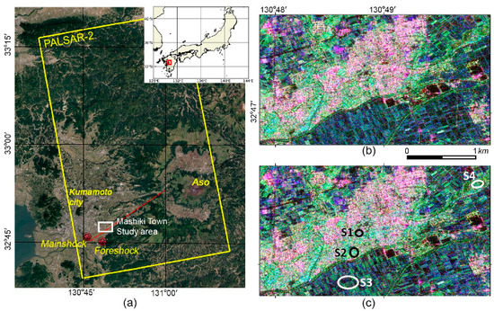
Figure 1.
(a) ALOS-2 PALSAR-2 data coverage (yellow rectangle) and location of the Mashiki Town study area (white rectangle) marked on the Google Earth, and PALSAR-2 images (red: HH; green: HV; blue: VV) of the study area acquired (b) before (3 December 2015) and (c) after (21 April 2016) the earthquake. Locations of the foreshock and mainshock of the 2016 Kumamoto earthquake are also marked in (a). The red dashed line in (a) illustrates the approximated location of the Futagawa fault where the major damages are distributed. Four regions of interest (S1: collapsed buildings; S2: intact buildings; S3: intact croplands; and S4: intact forests) are indicated in (c).
Figure 1b,c show the POLSAR data obtained under pre- and post-earthquake conditions of the main study area. Both data used in the study have the same acquisition geometry, and therefore changes in the data are directly related to the changes that occurred to the ground scatterers. By inspecting Google Earth’s historical satellite imagery, four regions of interest (S1 to S4 in Figure 1c) were manually selected to evaluate the earthquake-induced changes in the building areas and other natural scatterers. The selected regions of interest consist of collapsed buildings (S1), intact buildings (S2), intact croplands (S3), and intact forests (S4). The two images were coregistered and geocoded before analysis. In addition, polarimetric speckle filtering using the IDAN filter [12] was applied to reduce speckle effects.
3. Comparison of Pre- and Post-POLSAR Observables
The incidence wave of the POLSAR system has both horizontal (H) and vertical (V) polarization components. Each resolution cell of the POLSAR data is represented by a complex scattering matrix , such as
The elements in the complex scattering matrix depend on the geometric and dielectric properties of scatterers. In this section, we will discuss how to emphasize building-damaged areas from changes in the POLSAR data obtained under pre- and post-earthquake conditions.
3.1. Scattering Power Chnages
One of the fundamental SAR observables describing the scattering characteristics of the object is the scattering power or scattering coefficient, such as with . Then, the temporal change of the scattering power at -polarization channel can be obtained by the log ratio, such as
In the monostatic backscattering case, when by the scattering reciprocity, we have two co-polarization differences ( and ) and one cross-polarization difference () to characterize possible changes in the ground scatterers. Figure 2 shows the histogram of , , and for the selected regions of interest. The HH power is slightly reduced by the collapse of buildings and the VV power is slightly increased. However, it can be seen that and in the damaged areas are not distinct compared to other natural changes, particularly in croplands. The scattering power changes in intact areas are more noticeable in the cross-polarization channel, and therefore it is difficult to highlight the damaged areas using .
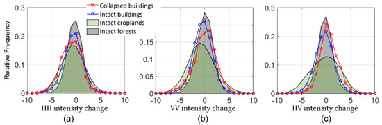
Figure 2.
Histograms of scattering power changes in (a) HH-, (b) VV-, and (c) HV-polarization channels.
The scattering matrix observation allows the characterization of scatterers not only for the H and V polarization states but also for any polarization basis through a unitary transformation [13]. Therefore, we can exploit backscattering intensities for different combinations of transmit/receive polarization states, named the polarization synthesis [14], which can better distinguish damaged areas. The polarization states of a wave can be characterized by the orientation and the ellipticity angles. The ellipticity angle corresponds to linear polarization states (e.g., H-polarization with and V-polarization with ). The ellipticity of and correspond to left circular (L) and right circular (R) polarization states, respectively. The polarization response plot [14] represents variation in scattering powers as a function of the orientation and ellipticity angles of the transmitted wave. Among the possible selection of the receiver polarization, co-polarization configuration, i.e., the transmitting and receiving antennas have the same polarization state, was considered in this study. Based on the scattering matrix observation, the co-polarization response can defined by [13]:
where, and .
Figure 3 shows averaged obtained at pre- and post-earthquake conditions for building-damaged areas. The at the pre-earthquake condition shows two minimum values at linear polarization oriented at (-linear) and maximum value at H polarization states. After the earthquake, the co-polarization response is changed, and the magnitude of scattering power changes can vary depending on the polarization states. According to the changes of co-polarization response shown in Figure 3c, the maximum increase and decrease of co-polarization response can be obtained at -linear and circular polarization states, respectively. Figure 4 shows the histogram of at -linear polarization states, and left and right circular polarization states for all selected regions of interest. It is seen that scattering power changes represented at -linear and circular polarization states can better separate collapsed buildings from other natural changes than the H–V basis cases shown in Figure 2.
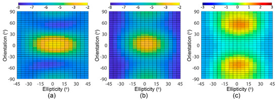
Figure 3.
Co-polarization response plots for building-damaged areas at (a) pre- and (b) post-earthquake conditions, and (c) difference between polarization responses.
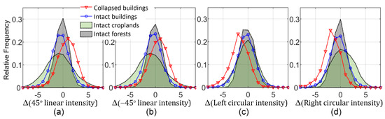
Figure 4.
Histograms of scattering power changes at (a) -linear, (b) -linear, (c) left circular, and (d) right circular polarization states.
3.2. Matrix Dissimilarity Measure
Changes in the POLSAR data between pre- and post-earthquake conditions can be also examined by measuring dissimilarity between the two polarimetric observation matrices. Based on the scattering matrix observation, the scattering properties of distributed scatterers can be described by the covariance matrix , defined by the complex scattering vector as follows:
Several methods [15,16,17,18] have been proposed to measure statistical similarity between two sample covariance matrices and acquired at before and after the earthquake, respectively. One of the widely used methods is the likelihood-ratio (LR) test of two acquisitions [15]. Two dissimilarity measures, such as the Bartlett distance () and the revised Wishart distance () can be derived from the LR test defined by the complex Wishart distribution [16,17], such as:
where and and denote the determinant and trace of a matrix, respectively. If both data are identical, the two distances and are equal to 0.
In addition to the statistical distance measures between the two distributions, another approach, named polarimetric similarity parameter [19,20], was proposed to examine differences between the scattering mechanisms of the temporal POLSAR observations. Using the correlation-based similarity measure, the polarimetric similarity parameter between two coherency matrices and acquired before and after the earthquake, respectively, can be written as:
where the coherency matrix and its line-of sight rotation can be defined from the Pauli-based scattering vector , such as [13].
The unitary rotation matrix is given by:
where is the orientation angle of a scatterer [21]. It can be estimated from the observed coherency matrix by the following relation:
Unlike LR-based distances and , is bounded to between 0 (maximum dissimilarity) to 1 (identical).
Figure 5 shows the histogram of dissimilarity measures , , and for the selected regions of interest. It is seen that the statistical distances between temporal covariance matrices ( and ) increase in areas where buildings were collapsed by the earthquake, but the increase of distances can be also observed by natural variations in croplands. On the other hand, the correlation-based dissimilarity measure shows significantly different values for collapsed buildings in comparison with those in other intact areas. One of the differences between the two types of dissimilarity measures is that the correlation-based measure is invariant to arbitrary scaling of the coherency matrix. Therefore, highlights temporal changes of polarimetric information regardless of the corresponding differences in overall amplitudes. The results shown in Figure 5 indicate that it is important to measure changes in the scattering mechanisms rather than the scattering amplitudes for effectively highlighting earthquake-induced changes.
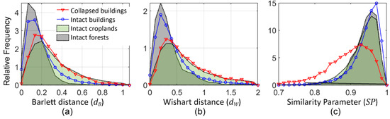
Figure 5.
Histograms of matrix dissimilarity measures: (a) the Bartlett distance (), (b) the revised Wishart distance (), and (c) the polarimetric similarity parameter.
3.3. Earthquake-Induced Scattering Mechanism Changes
The backscattered signal observed by the SAR system is a mixture of waves scattered from elementary scattering mechanisms within a resolution cell. To evaluate different scattering contributions in the observed signal, we first recall the scattering power decomposition technique proposed by Yamaguchi et al. [22]. The coherency matrix after orientation compensation can be assumed to be a linear combination of four elementary scattering models as follows:
where , , , and are surface, double-bounce, volume, and helix scattering contributions, and and are unknown double-bound and surface scattering coefficients to be estimated from the observed coherency matrix, respectively. The scattering powers , , , and corresponding to surface, double-bounce, volume, and helix scattering components, respectively, are determined by:
Figure 6 shows averaged , , , and scattering powers estimated from the coherency matrices and for the selected regions of interest. In the S1 site, the dominant scattering mechanism in the pre-earthquake condition is the double-bounce scattering followed by the surface and volume scattering components. Under the condition after the collapse of buildings in this area, the double-bounce component is reduced significantly while other scattering mechanisms are relatively increased. Changes in scattering components can be also observed in other non-damaged regions. However, no significant change in the double-bounce scattering contribution is found, as in the damaged areas. Consequently, the double-bounce scattering component of the scattering power decomposition can be used as an indicator for detecting the damaged areas.
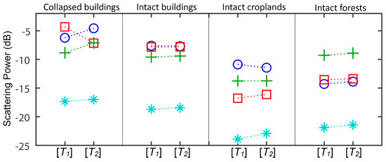
Figure 6.
The surface (blue-circle symbol), double-bounce (red-square symbol), volume (green-cross symbol), and helix (cyan-star symbol) scattering contributions of the scattering power decomposition for the selected regions of interest.
In order to emphasize the earthquake-induced variations in scattering mechanisms, two parameters corresponding to changes of the double-bounce scattering power () and the double-bounce scattering contribution among total received signals () can be defined as follows:
where is the total power of the radar return.
The scattering power decomposition provides useful information for interpreting different scattering mechanisms. However, since there can be many different ways to fit simple models to the observed matrix, estimation of the double-bounce scattering mechanism cannot be uniquely determined [23]. Instead of fitting elementary scattering models to the measurement matrix, there is an alternative way to expand the observed coherency matrix as a sum of elementary components using eigenvector decomposition [24] as follows:
where and are eigenvalues and eigenvectors of , respectively. It expands observed into the sum of three uncorrelated matrices where the eigenvalues () are the statistical weights for the three components. An eigenvector for each scattering contribution can be parameterized [24] as:
An important observation following from this decomposition is that the parameter can be a continuous measure of the type of scattering process of the scatterer independently of its orientation. It ranges from for isotropic surface scattering, to for isotropic dihedral or helix scattering. In order to analyze variations in the scattering mechanisms caused by the earthquake using of the three eigenvectors, two parameters indicating the change of the mean scattering mechanism () and the change of the dominant scattering mechanism () can be defined as follows:
Figure 7 shows the histogram of scattering mechanism indicators , , , and for the selected regions of interest. Compared with statistical distance and matrix similarity measures, all proposed parameters indicating variations of scattering mechanisms can better separate collapsed buildings from other intact areas. Selected scattering mechanism parameters commonly indicate a significant reduction of the double-bounce scattering mechanisms in damaged areas, while there are no apparent changes in scattering mechanisms in other areas.
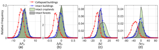
Figure 7.
Histograms of the scattering mechanism indicators: (a) the double-bounce scattering power (), (b) the double-bounce scattering contribution among total received signals (), (c) the mean scattering mechanism (), and (d) the change of the dominant scattering mechanism ().
4. Detection of Building-Damaged Areas from POLSAR Observables
4.1. Selection of Damage Indicator
In the previous section, we evaluated different polarimetric change indicators for discriminating collapsed areas from other type of changes using several manually selected regions of interest. It is seen that some change indicators, such as the changes of polarimetric scattering powers at -linear and circular polarization states, the coherency matrix similarity parameter, and the changes of double-bounce scattering mechanisms, can be useful to highlight damaged areas. For mapping building-damaged areas using POLSAR data, we first selected optimal parameters to be used in developing automatic detection algorithm among these polarimetric change indicators.
In order to compare detectability of different polarimetric change indicators independently of the detection methods, the ROC (receiver operating characteristic) analysis is carried out as shown in Figure 8. The ROC curve can be constructed by plotting the detection rate against the false-alarm rate at various thresholds. Given a threshold for a change indicator, the detection rate is determined by the ratio of the pixels detected as the changed class out of all pixels in the S1 site. The false-alarm rate is calculated similarly by the ratio of the pixels classified as the unchanged class out of all undamaged sites S2, S3, and S4.
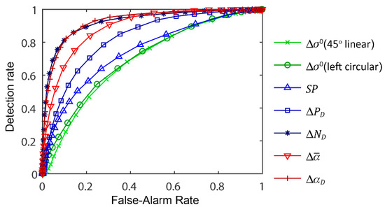
Figure 8.
The receiver operating characteristic curves for selected polarimetric change indicators.
The ROC curve for each polarimetric change indicator shows that the scattering mechanism indicators, particularly the dominant scattering mechanism , provide high detectability of damaged areas. This result represents that areas related to the building damages can be uniquely characterized as the dominant scattering mechanism shift from high values in undamaged conditions to low values after the earthquake. In addition to the dominant scattering mechanism, the changes of the double-bounce scattering component of the scattering power decomposition provide high detection performance. Particularly, the relative contribution of the double-bounce scattering mechanism among total received signals can better characterize the scattering mechanism variations existing in the building-damaged area than the double-bounce scattering power, which can be sensitive to other factors, such as the scatterers’ dielectric and geometric properties, number densities of vegetation constituents, and so on. Consequently, we selected and as damage indicators for automatically detecting building damages from POLSAR data.
4.2. Automatic Damage Detection
4.2.1. Binary Classification by Thresholding
As discussed above, it is possible to map building-damaged areas by distinguishing areas of low values from other areas in the damage-highlight images or . A map can be obtained by assigning each pixel of the damage-highlight images to either damaged class or undamaged background class . One of the simple and unsupervised ways to perform a binary decision is to set the threshold value in the difference image. In this study, we selected three widely used threshold selection methods, such as the Otsu [25], KI [26], and EM [27] methods, to obtain the binary classification map for damaged areas. The Otsu and KI methods set threshold values of the histogram of the image by minimizing the within-class variance of the two groups and by minimizing the average classification error rate, respectively. The EM method iteratively estimates a priori probabilities and Gaussian density functions and selects the threshold value according to the Bayes rule for minimum error. In order to assess the detection result quantitatively, several accuracy metrics are considered including the detection rate, false-alarm rate, Kappa coefficient (Kappa) [28], and figure of merit (FOM) [29].
Table 1 shows the accuracy analysis results for each binary classification result obtained by the Otsu, KI, and EM thresholding methods. According to the Kappa and FOM accuracy metrics, which provide overall ideas of detectability, the EM method provides the best detection accuracy among three thresholding methods. However, two kinds of problems can occur in the detection method of dividing the image into two groups using a single fixed threshold value. The first is that even in the EM method, providing the best performance exhibits a relatively low detection rate of less than about 40%. The second is that the threshold values can vary from region to region, showing different joint probability distributions.

Table 1.
Detection accuracies for the different polarimetric parameters.
4.2.2. Fuzzy-Based Contextual Classification
One possible way to solve this vagueness of decision boundary between damaged and undamaged classes is to use the fuzzy set theory [30]. The damaged class and the undamaged class can be considered as the fuzzy set. Each element in the observation space can be defined by the membership grades to class , i.e., . In order to apply fuzzy concepts to our detection problem, it is essential to determine the membership grades of each damage-highlight parameter or , such as and .
The membership grade depends on the problem to be solved, and, in practice, the membership generation is usually performed using training sets for the classes of interest of the particular data. Since the use of training data is difficult to use for the disaster application, the class conditional probability density functions estimated by the EM method are used for unsupervised construction of the membership grades. Each element of X is mapped to the membership grades based on the pairwise membership functions for damaged and undamaged classes and as illustrated in Figure 9. In this study, simple piecewise linear functions are used for the membership functions, defined as:
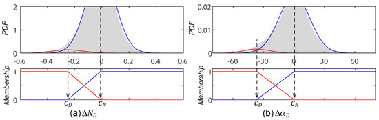
Figure 9.
Construction of fuzzy membership functions for the damaged (red) and undamaged (blue) classes in each damage indicator (a) and (b) .
The two parameters and determine the shape of the membership functions. In this study, and can be determined by EM-based estimation of the mean of Gaussian conditional distributions for the damaged and undamaged classes, respectively.
Although the two independent polarimetric parameters and provide information on building damages, they convey slightly different scattering properties of scatterers and may show different sensitivity to natural changes occurring in the undamaged areas. Consequently, we can exploit the synergy of the two polarimetric information in identifying building-damaged areas. Another advantage of using the fuzzy set theory is that it can be used as a mathematical tool to facilitate data fusion. The fuzzified information of each polarimetric parameter can be easily combined through the fuzzy operators [30]. Since the two polarimetric parameters indicate similar information in different views, the conjunctive operator can be used for retrieving reliable information among the two agreeing parameters. The combined fuzzy membership grade can be generated by the fuzzy AND operator as:
Since the fuzzed membership grade is determined exclusively by the pixel values, it may still provide noisy detection results. To further improve the detection performance, the spatial contextual information can be considered in the binary classification. One of the simple ways to consider the local spatial information in the classification process is an iterative updating of class membership grades using the local neighborhood of the pixel under consideration. In this study, we adopted iterative contextual membership updating by the average operator given in [31]. The initial membership grade determined by (21), the contextual membership grade of the pixel under consideration at (t + 1) iteration is given by:
where is the number and is the membership grades of the local neighborhood system. In order to avoid an over-smoothened membership grade, the contextual membership updating applied only to pixels that do not obviously belong to either class by using the quadratic fuzzy entropy [32], which is a measure of fuzziness, defined as:
After updating the contextual membership grade, we can obtain a hard membership grade to make a binary classification map. The pixel value of the classification map at (t + 1) iteration can be generated accordingly with the following decision rule.
The iteration stops when the percentage of newly labeled pixels becomes smaller than 0.1%.
Figure 10 shows the membership grades of each polarimetric parameter, fuzzed and contextual membership grades, and the binary classification result from the iterative contextual fusion. A Google Earth optical image is also shown for reference. The blue-outlined area indicates the urban district and the red ellipse illustrates the areas where many damaged buildings can be visually identified in the optical image. It is seen that the building-damaged area is more emphasized by the fusion of polarimetric parameters based on fuzzy set theory, and false alarms in agricultural areas unrelated to building damage are significantly reduced. The binary decision result by the contextual fusion shown in Figure 10e provides significantly improved detection performance for the selected area of interest with the detection rate of 90.9%, false-alarm rate 1.3%, Kappa of 81.3%, and FOM of 69.7% as listed in Table 2.
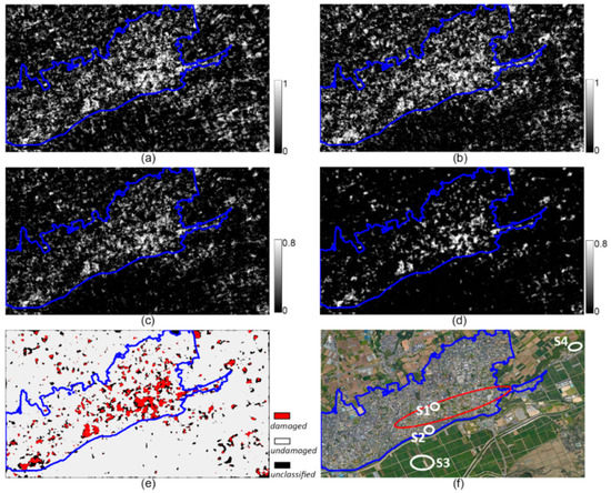
Figure 10.
Determined fuzzy membership grades of each damage indicator (a) and (b) . The combined membership grade by (c) fuzzy membership fusion and (d) spatial contextual fusion. (e) The binary classification result from the contextual fusion. (f) Reference Google Earth optical image of the study area.
Table 2.
Detection accuracies of the fuzzy contextual classification result.
5. Discussion
5.1. Comparison with the Single-Polarization Damage Detector
Although the fully polarimetric data provides several advantages in extracting physical quantities of the scattering targets, most of the SAR systems which have full polarization capability are often operated in single- or dual-polarimetric modes to meet various operational requirements on the resolution and coverages. In this section, we examined the performance of the single-polarization detector in [1,2,3,4] in comparison with the result obtained in this study.
The damage detector () in [4] was derived based on both the difference (d) and the correlation coefficient () between the HH-polarization backscatter images obtained under pre- and post-earthquake conditions. The former is defined in the same way as Equation (2), and the latter can be defined as follows:
where and are the scattering powers of the pre- and post-earthquake data, respectively. By combining these two change measures, the damage indicator -factor is proposed as:
It ranges from −0.5 to 1.5, where the high -factor indicates a high possibility of changes between the temporal SAR images.
Figure 11 shows the calculated -factor in comparison with one of the proposed change indicators, . While the polarimetric parameter highlights building-damaged areas in urban areas, the single-polarization -factor enhances both natural background changes and building damages. If we limit the detection problem to the blue-outlined urban area, the -factor can provide meaningful information about the building damages. Therefore, it is possible to use the single-polarization damage detector if the urban areas are extracted before applying it. If appropriate information on urban areas is not available, there can be a significant number of false alarms in the detection results as an increase of temporal baseline between the two SAR acquisitions. On the other hand, the polarimetric damage indicators can effectively highlight the building-damaged areas, by tracking the damage-induced changes of the scattering mechanism.
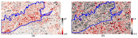
Figure 11.
Comparison of (a) fully polarimetric damage indicator () and (b) single-polarization damage indicator (-factor).
5.2. Grid-Based Damage Index and Comparison with In-Situ Survey
Most field investigations of damage to buildings have been carried out by a grid-based survey of damage degree of buildings. In the case of the 2016 Kumamoto earthquake, a field survey was carried by the Architectural Institute of Japan and the grid-based damage map was produced [33]. The damage status of buildings in each grid was visually inspected and categorized by Okada’s damage levels [34]. Figure 12 shows the grid-based damage map generated from the field survey report. The map shows the grid-based major damage rate (DR), which is the number of buildings belonging to major damage categories (damage levels 4 and 5) among the total number of buildings in each grid cell.
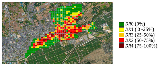
Figure 12.
The grid-based major damage rate (DR) by the field survey [33]. Five DR categories indicate the number of buildings belongs to major damage categories (damage levels 4 and 5 [34]) among the total number of buildings in each grid cell.
Figure 13 shows the grid-wise mean of the radar parameters with respect to the major damage rates. The Spearman’s rank correlation coefficient () is used to represent the correlation between the radar parameter and the survey result. Compared to the scattering-power-based change indicators, such as and -factor, the selected disaster indicators ( or ) show a higher correlation with the major damages assessed by the field survey. The fuzzy membership fusion can further increase the correlation between the SAR-derived damage index and the survey result. It is worth noting that the colors in the damage map are not the level of damages but the number density of the level-5 damaged buildings. On the other hand, the radar scattering parameter is a continuous random variable which may vary continuously depending on the degree of damage. In addition, due to the radar observation geometry and the structure of buildings, there can be a difference between the SAR pixel coordinate and the building footprint. Consequently, there are significant variabilities of grid-wise mean values of radar scattering parameters as the increase of the number of major damaged buildings in the survey grid-cell.
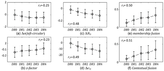
Figure 13.
Grid-wise mean of the radar parameters (a) , (b) z-factor, (c) , (d) , (e) and (f) with respect to the major damage rates from the field survey.
In order to generate a radar-based damage map corresponding to the major damage map of the field survey, a grid-based damaged pixel rate () can be calculated as:
where is the total number of pixels within the grid and is the binary classification result of pixel in the grid cell generated by the contextual fusion according to Equation (25). The size of the grid cell is set to match the field survey data.
Figure 14 shows the calculated damaged pixel rate ( in comparison with the from the field survey. It is seen that the two independent damage maps show a high correlation for the severely damaged areas. Note that corresponds to the areal density of damages, i.e., the rate of pixels corresponding to the damaged class among all pixels (approximately 11 × 11 pixels in this case) in a grid cell. On the other hand, the from the field survey indicates the number density of damaged buildings. Consequently, there are inherent differences between the two data sets, which can vary from grid to grid due to variations of the size and number of buildings between grid cells.
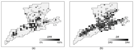
Figure 14.
(a) Damaged pixel rate (DPR) by synthetic aperture radar (SAR) data and (b) major damage rate (DR) by the field survey.
Figure 15 shows a comparison between and five damage categories of the survey data. For effective comparison, the is divided into five intervals and the ratios of categories corresponding to each interval are plotted on the stacked bar graph. Due to the characteristic difference between the two damage maps as well as the effect of registration noise, the relationship between and is not one to one. The tends to overestimate areas with a small number of damaged buildings and overestimate areas with many damaged buildings. Nonetheless, it is possible to notice an overall correspondence between the two damage maps. As the from SAR data increases, the ratio of the category decreases and the ratio of the category increases. The use of additional information on the number and area of buildings may produce results that are more consistent with field survey data. However, it should be pointed out that, significant correlation with field data derived from a completely different approach can only be obtained with the appropriate use of polarization information.
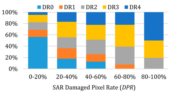
Figure 15.
Comparison of SAR-based damaged pixel rate (DPR) and survey-based major damage rate.
6. Conclusions
The repetitive observation of the earth’s surface with space-borne SAR remote sensing has shown great potential to detect a large damaged area caused by various natural disasters. In most approaches for detecting damaged areas using SAR images, the pre-disaster data obtained shortly before the event at the same imaging geometry with the emergency observation data are crucial to obtain successful detection results [35]. However, appropriate baseline data is not always available for unpredictable natural disasters. This study aimed to evaluate the usability of polarimetric SAR data in the detection of earthquake-induced building damages with the presence of significant natural changes. Different change augmentation approaches, such as the changes of polarimetric scattering powers, the matrix distance measures, and changes of the scattering mechanisms, were investigated in this study to derive optimal damage indicators for building damages. In addition, we proposed a novel change detection method by the fuzzy-based fusion of polarimetric damage indicators.
Experimental results for the Kumamoto earthquake with ALOS-2 PALSAR-2 data demonstrate a high potential of utilizing polarimetric scatter type indicators for identifying damaged areas in urban areas. The results indicate that, rather than using the average scattering mechanism of the full covariance matrix, it has been demonstrated experimentally that the use of scattering mechanisms associated with characteristic scattering phenomena in buildings can reduce false alarms in natural changes and improve detectability in building-damaged areas. Particularly, two polarimetric parameters, such as the double-bounce scattering contribution among total received signals and the dominant scattering mechanism, were selected as the building-damage indicators. In addition, an unsupervised fuzzy contextual classification algorithm was proposed for producing the damage map for build-damaged areas was proposed. The pixel-based accuracy analysis results showed that the proposed automatic damage map can successfully detect the manually selected damaged areas with a detection rate of about 90.9% and false-alarm rate of about 1.3%.
We also compared the grid-based damage map produced by the proposed approach with the damage map from the field survey. Despite inherent differences between the two damage maps, significantly damaged and undamaged areas in the survey data can be also successfully identified by the SAR-based damage map. However, the relationship between the SAR-based damage rate and the major damage rates in the survey data is not one to one, particularly in a mixed area of damaged and intact buildings. The performance of damage assessment can be improved if the additional information on buildings in urban areas are used in the classification chain. However, in general, urban thematic information such as urban distribution, density, and structural features are not globally available. Therefore, for operational and rapid detection, and evaluation of disaster areas, we will mainly focus on improving the SAR-based damage evaluation algorithm in our future study by retrieving structural information on buildings from the baseline data. In addition, to improve the ability to distinguish the level of building damages and to detect earthquake-induced small scale displacements other than building damages, the integrated use of polarimetric and interferometric techniques will be investigated.
Author Contributions
Conceptualization, S.-E.P.; Methodology, software, formal analysis, and writing—original draft preparation, S.-E.P.; validation, formal analysis writing—review & editing, Y.T.J.; Project administration, Y.T.J. All authors have read and agreed to the published version of the manuscript.
Funding
This work was supported by the “Satellite Information Application” program of the Korea Aerospace Research Institute (KARI) and by the MSIT (Ministry of Science and ICT), Korea, under the ITRC (Information Technology Research Center) support program (IITP-2017-2016-0-00288) supervised by the IITP (Institute for Information & Communications Technology Promotion).
Acknowledgments
The authors are grateful to JAXA for providing ALOS-2 PALSAR-2 data.
Conflicts of Interest
The authors declare no conflicts of interest.
References
- Matsuoka, M.; Yamazaki, F. Use of satellite SAR intensity imagery for detecting building areas damaged due to earthquakes. Earthq. Spectra 2004, 2, 975–994. [Google Scholar] [CrossRef]
- Matsuoka, M.; Yamazaki, F. Building damage mapping of the 2003 Bam, Iran, earthquake using Envisat/ASAR intensity imagery. Earthq. Spectra 2005, 21, 285–294. [Google Scholar] [CrossRef]
- Matsuoka, M.; Yamazaki, F.; Ohkura, H. Damage mapping for the 2004 Niigata-ken Chuetsu earthquake using Radarsat images. In Proceedings of the 2007 Urban Remote Sensing Joint Event, Paris, France, 11–13 April 2007. [Google Scholar]
- Liu, W.; Yamazaki, F. Extraction of collapsed buildings in the 2016 Kumamoto earthquake using multi-temporal PALSAR-2 data. J. Disaster Res. 2017, 12, 241–250. [Google Scholar] [CrossRef]
- Chini, M.; Pierdicca, N.; Emery, W.J. Exploiting SAR and VHR optical images to quantify damage caused by the 2003 Bam earthquake. IEEE Trans. Geosci. Remote Sens. 2009, 47, 145–152. [Google Scholar] [CrossRef]
- Dekker, R. High-resolution radar damage assessment after the earthquake in Haiti on 12 January 2010. IEEE J. Sel. Top. Appl. Earth Obs. Remote Sens. 2011, 4, 960–970. [Google Scholar] [CrossRef]
- Park, S.-E.; Yamaguchi, Y.; Kim, D.J. Polarimetric SAR remote sensing of the 2011 Tohoku earthquake using ALOS/PALSAR. Remote Sens. Environ. 2013, 132, 212–220. [Google Scholar] [CrossRef]
- Chen, S.-W.; Sato, M. Tsunami damage investigation of built-up areas using multitemporal spaceborne full polarimetric SAR images. IEEE Trans. Geosci. Remote Sens. 2013, 51, 1985–1997. [Google Scholar] [CrossRef]
- Chen, S.-W.; Wang, X.-S.; Sato, M. Urban damage level mapping based on scattering mechanism investigation using fully polarimetric SAR data for the 3.11 East Japan earthquake. IEEE Trans. Geosci. Remote Sens. 2016, 54, 6919–6929. [Google Scholar] [CrossRef]
- Kato, A.; Nakamura, K.; Hiyama, Y. The 2016 Kumamoto earthquake sequence. Proc. Jpn. Acad. Ser. B 2016, 92, 358–371. [Google Scholar] [CrossRef]
- 2016 Kumamoto Earthquake Verification Report of Correspondence by Mashiro-Machi. Available online: https://www.town.mashiki.lg.jp/bousai/kiji0032410/3_2410_1633_up_j7cvpcog.pdf (accessed on 30 September 2019). (In Japanese).
- Vasile, G.; Trouve, E.; Lee, J.-S.; Buzuloiu, V. Intensity-driven adaptive neighborhood technique for polarimetric and interferometric SAR parameters estimation. IEEE Trans. Geosci. Remote Sens. 2006, 44, 1609–1621. [Google Scholar] [CrossRef]
- Lee, J.S.; Pottier, E. Polarimetric Radar Imaging—From Basics to Applications; CRC Press: Boca Raton, FL, USA, 2009. [Google Scholar]
- Van Zyl, J.J.; Zebker, H.A.; Elachi, C. Imaging radar polarization signatures: Theory and observation. Radio Sci. 1987, 22, 529–543. [Google Scholar] [CrossRef]
- Conradsen, K.; Nielsen, A.A.; Schou, J.; Skriver, H. A test statistic in the complex Wishart distribution and its application to change detection in polarimetric SAR data. IEEE Trans. Geosci. Remote Sens. 2003, 41, 4–19. [Google Scholar] [CrossRef]
- Kersten, P.R.; Lee, J.-S.; Ainsworth, T.L. Unsupervised classification of polarimetric synthetic aperture radar images using fuzzy clustering and EM clustering. IEEE Trans. Geosci. Remote Sens. 2005, 43, 519–527. [Google Scholar] [CrossRef]
- Anfinsen, S.N.; Jenssen, R.; Eltoft, T. Spectral clustering of polarimetric SAR data with Wishart-derived distance measures. In Proceedings of the POLInSAR 2007, Esrin, Italy, 22–26 January 2007. [Google Scholar]
- Frery, A.C.; Nascimento, A.D.C.; Cintra, R.J. Analytic expressions for stochastic distances between relaxed complex Wishart distributions. IEEE Trans. Geosci. Remote Sens. 2014, 52, 1213–1226. [Google Scholar] [CrossRef]
- Yang, J.; Peng, Y.; Lin, S. Similarity between two scattering matrices. Electron. Lett. 2001, 37, 193–194. [Google Scholar] [CrossRef]
- An, W.; Zhang, W.; Yang, J.; Hong, W. Similarity between two targets and its application to polarimetric target detection for sea area. In Proceedings of the 24th PIERS, Cambridge, MA, USA, 1–6 July 2008; pp. 515–520. [Google Scholar]
- Lee, J.-S.; Schuler, D.L.; Ainsworth, T.L.; Krogager, E.; Kasilingam, D.; Boerner, W.-M. On the estimation of radar polarization orientation shifts induced by terrain slopes. IEEE Trans. Geosci. Remote Sens. 2002, 40, 30–41. [Google Scholar]
- Yamaguchi, Y.; Sato, A.; Boerner, W.M.; Sato, R.; Yamada, H. Four-component scattering power decomposition with rotation of coherency matrix. IEEE Trans. Geosci. Remote Sens. 2011, 49, 2251–2258. [Google Scholar] [CrossRef]
- Cloude, S.R. Polarisation: Applications in Remote Sensing; Oxford University Press: New York, NY, USA, 2010. [Google Scholar]
- Cloude, S.R.; Pottier, E. A review of target decomposition theorems in radar polarimetry. IEEE Trans. Geosci. Remote Sens. 1996, 34, 498–518. [Google Scholar] [CrossRef]
- Otsu, N. A threshold selection method from grey level histograms. IEEE Trans. Syst. Man Cybern. 1979, 9, 62–66. [Google Scholar] [CrossRef]
- Kittler, J.; Illingworth, J. Minimum error thresholding. Pattern Recognit. 1986, 19, 41–47. [Google Scholar] [CrossRef]
- Bruzzone, L.; Prieto, D.F. Automatic analysis of the difference image for unsupervised change detection. IEEE Trans. Geosci. Remote Sens. 2000, 38, 1171–1182. [Google Scholar] [CrossRef]
- Cohen, J. A coefficient of agreement for nominal scales. Educ. Psychol. Meas. 1960, 20, 37–46. [Google Scholar] [CrossRef]
- Foulkes, S.B.; Dooth, D.M. Ship detection in ERS and Radarsat imagery using a self-organising Kohonen neural network. In Proceedings of the Nova Scotia Conference on Ship Detection in Coastal Waters, Digby, NS, Canada, 31 May–1 June 2000. [Google Scholar]
- Zadeh, L.A. Fuzzy sets. Inf. Control 1965, 8, 338–353. [Google Scholar] [CrossRef]
- Solaiman, B.; Pierce, L.; Ulaby, F. Multisensor data fusion using fuzzy concepts: Application to land-cover classification using ERS-1/JERS-1 SAR composites. IEEE Trans. Geosci. Remote Sens. 1999, 37, 1316–1326. [Google Scholar] [CrossRef]
- Fauvel, M.; Chanussot, J.; Benediktsson, J.A. Decision fusion for the classification of urban remote sensing images. IEEE Trans. Geosci. Remote Sens. 2006, 44, 2828–2838. [Google Scholar] [CrossRef]
- National Institute for Land and Infrastructure Management (NILIM), Quick Report of the Field Survey on the Building Damage by the 2016 Kumamoto Earthquake, Technical Note No.929. Available online: http://www.nilim.go.jp/lab/bcg/siryou/tnn/tnn0929.htm (accessed on 30 September 2019). (In Japanese).
- Okada, S.; Takai, N. Classifications of structural types and damage patterns of buildings for earthquake field investigation. In Proceedings of the 12th World Conference on Earthquake Engineering, Auckland, New Zealand, 30 January–4 February 2000. [Google Scholar]
- Plank, S. Rapid Damage Assessment by Means of Multi-Temporal SAR–A Comprehensive Review and Outlook to Sentinel-1. Remote Sens. 2014, 6, 4870–4906. [Google Scholar] [CrossRef]
© 2020 by the authors. Licensee MDPI, Basel, Switzerland. This article is an open access article distributed under the terms and conditions of the Creative Commons Attribution (CC BY) license (http://creativecommons.org/licenses/by/4.0/).