Abstract
Subsurface targets can be detected from space-borne sensors via archaeological proxies, known in the literature as cropmarks. A topic that has been limited in its investigation in the past is the identification of the optimal spatial resolution of satellite sensors, which can better support image extraction of archaeological proxies, especially in areas with spectral heterogeneity. In this study, we investigated the optimal spatial resolution (OSR) for two different cases studies. OSR refers to the pixel size in which the local variance, of a given area of interest (e.g., archaeological proxy), is minimized, without losing key details necessary for adequate interpretation of the cropmarks. The first case study comprises of a simulated spectral dataset that aims to model a shallow buried archaeological target cultivated on top with barley crops, while the second case study considers an existing site in Cyprus, namely the archaeological site of “Nea Paphos”. The overall methodology adopted in the study is composed of five steps: firstly, we defined the area of interest (Step 1), then we selected the local mean-variance value as the optimization criterion of the OSR (Step 2), while in the next step (Step 3), we spatially aggregated (upscale) the initial spectral datasets for both case studies. In our investigation, the spectral range was limited to the visible and near-infrared part of the spectrum. Based on these findings, we determined the OSR (Step 4), and finally, we verified the results (Step 5). The OSR was estimated for each spectral band, namely the blue, green, red, and near-infrared bands, while the study was expanded to also include vegetation indices, such as the Simple Ratio (SR), the Atmospheric Resistance Vegetation Index (ARVI), and the Normalized Difference Vegetation Index (NDVI). The outcomes indicated that the OSR could minimize the local spectral variance, thus minimizing the spectral noise, and, consequently, better support image processing for the extraction of archaeological proxies in areas with high spectral heterogeneity.
1. Introduction
Since the launch of the first commercial high-spatial-resolution multispectral satellite sensor, namely the IKONOS, archaeological prospection surveys systematically explored spaceborne optical-based observations [1,2]. IKONOS, GeoEye, QuickBird, WorldView, Gaofen, and other satellites are some of the sensors which have been used in the past, in different geographical regions of the world [1,3,4,5].
To better understand an archaeological landscape, a particular focus that has attracted the interest of the scientific community was the exploitation of such space-based observations for the detection of shallow buried remains. The latest can be achieved through the detection of archaeological proxies, known in the literature as cropmarks [6,7,8]. Such archaeological proxies (cropmarks) detected in satellite images can be used to map and detect subsurface archaeological remains at shallow depths.
Detection of cropmarks has been already studied in the past, mainly through the analysis of medium and high-resolution satellite imageries [9,10,11,12], while multi-temporal satellite image analysis has also been recently introduced [13,14]. Cropmarks are usually formed in areas where vegetation overlay shallow-buried archaeological remains. The latest is responsible for retaining a different percentage of soil moisture compared to the rest of the crops cultivated in an area. As [15] stated, depending on the type of the buried archaeological features, crop vigor may be enhanced or reduced.
Several researches tend to agree that such archaeological proxies have been limited studied mainly due to their complexity: several parameters should be taken into consideration, such as the characteristics of the buried features, the burial depth of them, soil characteristics, climatic and environmental parameters, cultivation techniques, etc. [16,17,18]. Furthermore, moisture availability and the availability of dissolved nutrients to the crops (at crucial growing times and periods for the plant) are also important parameters that need to be considered.
Traditionally, the selection of the most appropriate satellite sensor able to better detect subsurface archaeological remains has relied mostly on budget restrictions and available funds, image availability, cloud coverage, etc. Indeed, this is the current practice followed in many prospection surveys; however, it is evident that each spaceborne sensor shares different spectral characteristics and spatial resolutions. While the former has been already discussed in the literature concerning the detection of archaeological proxies [19], studies dealing with spatial resolution are still lacking.
The observation scale, linked with the spatial resolution of an image (pixel size), is one of the essential characteristics of the image processing chain (beyond the spectral resolution) followed in the prospection surveys since it can support visual interpretation (as an interpretation key) and extraction of archaeological proxies. Observation scale can vary according to the characteristics of each case study area, due to its unique spatial and spectral characteristics. In areas, with high spectral heterogeneity, the extraction of archaeological proxies can be problematic and challenging.
The importance of an optimum observation scale has long been studied in the literature, mainly for environmental sciences and applications, also triggered by the increased capabilities of spaceborne and airborne remote sensing sensors [20]. The term “scale” can have different meanings spanning from the pixel resolution, the cartographic scale, the modeling scale and the geographic scale, while it has also been misinterpreted with the spatial extent and the coverage of the area of interest. While optimum observation scale is of fundamental importance for several scientific disciplines, in the domain of archaeological prospection, there has been limited discussion on this. It is, therefore, not strange to see a growing number of the exploitation of new high-resolution satellite imageries, thus providing sub-meter resolution products, following the trend of the technological changes in the space sector. Nevertheless, the use of high-resolution datasets is not always the optimum scale of observation, as the variance of the datasets might also be increasing the noise and the outcomes of the products.
Studies for the selection of the appropriate observation scale (pixel size) has been already presented in other disciplines, exploiting earth observation data [20,21]. For instance, optimal spatial resolution for obtaining maximum coverage of algal blooms without losing key details necessary for adequately monitoring bloom concentrations was presented in [22], while optimal spatial resolutions for the detection and discrimination of coniferous classes in a forested environment can be found in [23]. However, similar studies for the detection of the optimum spatial resolution, capable of detecting and discriminating archaeological proxies, for supporting archaeological prospections studies has been incompletely discussed.
The identification of the optimal spatial resolution (OSR) can be defined based on image statistics and local mean-variance values. The local variation value can act as the indicator of the optimal spatial resolution in cases of spectral heterogeneity, as this has been already presented in the past [21]. The local variance method, used as an indicator of the OSR, measures the relationship between the size of the targets under investigation (e.g., archaeological proxies) in a specific spatial resolution and then calculates the mean value of the standard deviation on successively spatially degraded image upscaling. This step is repeated to retrieve a new degraded image. Based on the results, the optimal spatial resolution is set when the local mean-variance is minimized. Therefore, the OSR corresponds to the observation scale (pixel size), which provides the minimal variance of the area under investigation. While OSR is also linked with the spatial dimensions of each target (using as a rule of thumb the half-pixel size according to the dimensions of the target), this needs to be investigated further, especially when the area of investigation shares a spectral complexity (mixed pixels) [22].
As the estimation of the OSR value is related to the spectral characteristics of the area under investigation, and the archaeological proxies’ properties, this study aimed to present the overall methodology and framework, which can be transferred and implemented in other areas. For this reason, the current study presents the results for the identification of the OSR for two specific case studies. The first study concerns a simulation approach based on “pure” spectral libraries, while in the second case study, the high spectral heterogeneity of a real application is evaluated. The following section further explains the overall methodology and the steps that have been followed. The various materials and overall results are also presented below.
2. Materials and Methods
The optimum spatial resolution was investigated in two different case studies: (a) using ground spectral signatures over simulated buried archaeological targets (case study 1) and (b) using high-resolution WorldView-2 optical image over an existing archaeological site (case study 2). In both examples, the spectral resolution of the data was restricted into the visible and near-infrared part of the spectrum (400-900nm).
The scope behind the selection of these two different examples was to initially investigate the impact of the pixel resolution and the OSR working with “pure” spectral libraries, whereas noise and mixed spectral signatures are minimum. This experiment will allow us to move in areas with high spectral heterogeneity, such as the example of the second case study.
In the first example (case study 1), we used ground spectral signatures acquired from a hand-held spectroradiometer over simulated buried archaeological features [23]. In detail, in an experimental test site in the Alampra village, in Cyprus, different targets where physically buried and then cultivated on top with barley crops. Spectral signature measurements of barley crops recorded over these buried features were grouped as “archaeological proxies”, while spectral signatures taken at the rest of agricultural field were grouped under the category of “healthy vegetation”. Ground spectral signatures were taken during the whole phenological cycle of the crops; however, here we explore only the datasets from the optimum temporal window: based on previous statistical analysis conducted by [19], the optimum temporal window was determined during the beginning of the crops boot stage, since during this period, the spectral distance between the archaeological proxies and the rest cultivated area is maximized. For the collection of the ground spectral signatures, the GER-1500 (Spectra-Vista), a lightweight, single-beam field spectroradiometer measuring over the visible to near-infrared wavelength range (350–1050 nm), was used.
The spectral profile of these two categories, along with their standard deviations, are depicted in Figure 1. The line with red color indicates the spectral profile of the archaeological proxies (simulated “archaeological site”), while the line with blue color indicates the mean spectral signature for the healthy vegetation (“healthy site”). As shown, both spectral signatures have similar reflectance values and trend in the visible part of the spectrum (approximately from 400 up to 650 nm), while spectral differences can be observed in the near-infrared part of the spectrum, including also the red-edge part (approximately from 650–900 nm). The spectral regions of 700 nm and 800nm have also been reported in the literature [19] as the optimum spectral range for detecting archaeological proxies.
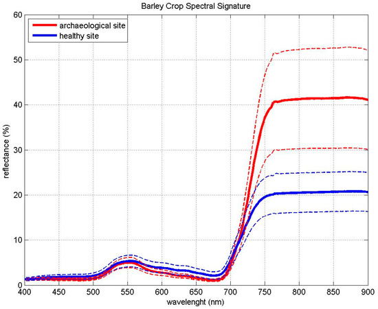
Figure 1.
Mean spectral signatures of archaeological proxies (archaeological site, red color) and healthy vegetation (healthy site, blue color) used in our study [19].
For the second case study, archaeological proxies have been identified within the archaeological site of “Nea Paphos”, Cyprus. In this case, a high-resolution WorldView-2 image (date of acquisition 10th of May 2015, Figure 2a) was used. The specific archaeological site was examined, since it shares a high spectral heterogeneity, with significant spectral variance between the various features [22]. This spectral confusion prohibits, therefore, the overall interpretation of the area. In addition, the selection of a fixed pixel resolution based exclusively on the spatial dimensions of the targets under investigation (also refer to Table 1 below) is problematic. Various features can be found in the archaeological site of “Nea Paphos”, such as the floor mosaics, soil from excavations activities, backfilled excavation trenches, mosaics protected from the atmosphere and weather conditions that may have been carefully covered, etc. Moreover, local bushes and shrubs can be found in parts of the site, while in other parts, no vegetation cover is observed.
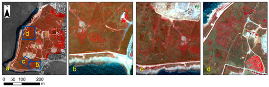
Figure 2.
The WorldView-2 multispectral image (2 m spatial resolution, date of acquisition 10th of May 2015) used for the second case study area. A general view and location of the various selected region of interests (ROIs) over the archaeological site of “Nea Paphos” are indicated in (a) ROI-1 indicating an elliptical shape (amphitheater?) in (b); various linear crop marks indicating ancient road network (?) in (c) and various crop marks at the western part of the site in (d).

Table 1.
Properties of the selected Regions of Interest (ROIs) at the archaeological site of Nea Paphos, Cyprus.
In the archaeological site of ‘Nea Paphos’, three region of interests (ROIs) have been further processed, including an area with an elliptical shape at the southern part of the site (ROI-1, Figure 2b), a north to south linear vegetation proxy, possible linked to ancient road network (ROI-2, Figure 2c), and a small linear and semi-circular archaeological proxies at the western part of the site (ROI-3, Figure 2d) The spatial extent of these ROIs is provided in Table 1.
The overall methodology to detect the optimum spatial resolution (OSR) comprises the following five (5) steps mentioned below, based on the work carried out by [20,21]:
- Step 1: Definition of the geographical entities under investigation. In our study, two groups of entities were investigated: (i) the simulated buried archaeological feature of case study 1 and (ii) the three ROIs of case study 2. The definition of these geographical entities is the most critical step of the overall methodology since the OSR results are linked directly with the selected features. A different selection of other entities will probably lead to new OSR values.
- Step 2: Determine the optimization criterion for the selection of the optimum spatial resolution. As mentioned earlier in this study, the local mean-variance was used as an indicator for the optimum spatial resolution. The OSR can be defined as the pixel size value was beyond that the mean-variance is increased due to the phenomenon of mixed pixels, once the feature under investigation starts to be integrated with the rest of the environment. Therefore, the minimal variance was used as the indicator of the optimal spatial resolution as this was also used in the past [23].
- Step 3: Spatially aggregation of the spectral datasets. For the first case study, the simulated dataset was gradually aggregated using a upscaling factor of 2, 3, 4, 5, and 10; for the second study, the image was aggregated with a upscaling factor of 3, 4, 5, 10, 15, and 30.
- Step 4: Identification of the optimum spatial resolution. Using the local mean-variance, the optimum spatial resolution was selected for each case study, based on the criterion set in Step 2. In cases where different OSR is identified for each spectral band, while an overall OSR is also estimated.
- Step 5: Verification of the results. The latest step includes the interpretation of the OSR results with the visual inspection of the aggregated images.
3. Results
3.1. Simulation Results—Case Study 1
Based on the spectral libraries from the handheld spectroradiometer, simulated computer-based images were created in the MATLAB R2016b environment. Table 2 shows the blue, green, red, and near-infrared bands of the simulated buried archaeological feature, drawn with a rectangular shape. This simulated feature is indicated with a red square at the centre of the figures of Table 2. The initial ground spectral signatures (Table 2, column a) were gradually aggregated to a pixel size of 2 (Table 2, column b), then to pixel size of 3 (Table 2, column c), after to a pixel size of 4 (Table 2, column d), to a pixel size of 5 (Table 2, column e), and finally to a pixel size of 10 (Table 2, column f).
Table 2.
(a) Blue, green, red, and near-infrared bands from simulated dataset pixel size 1; (b) blue, green, red, and near-infrared bands from simulated dataset pixel size 2; (c) blue, green, red, and near-infrared bands from simulated dataset pixel size 3; (d) blue, green, red, and near-infrared bands from simulated dataset pixel size 4; (e) blue, green, red, and near-infrared bands from simulated dataset pixel size 5; and (f) blue, green, red, and near-infrared bands from simulated dataset pixel size 10.
The value of pixel size refers to the level of units (pixels) rather than actual meters since the image is a simulated product derived from the interpolation of spectral signatures in a computer-based environment. However, for unit purposes, it should be mentioned that the spectroradiometric measurements taken with a lens of 4° Field Of View (FOV), thus covering an area of approximately 10 × 10 cm at a ground level, which can be considered as the basis for the first observation level (pixel size 1). Consequently, a pixel size of 2 refers to an area of 20 × 20 cm, a pixel size of 3 refers to an area of 30 × 30 cm, a pixel size of 4 refers to an area of 40 × 40 cm, a pixel size of 5 refers to an area of 50 × 50 cm, and finally, a pixel size of 10 refers to an area of 100 × 100 cm.
Based on the visual interpretation of the Table 2, it is clear that the simulated buried target is visible (to some extent) to all pixel sizes and for all spectral bands; however, not all images allow the interpretation of the rectangular shape of the simulated archaeological feature. In addition, differences between the wavelengths’ ranges do exist, since the red and the near-infrared bands (Table 2, row 3,4) tend to give the highest contrast between the buried feature and the surrounding area. This was expected since, as mentioned earlier, this range of wavelength is the most appropriate for monitoring vegetation cover [19].
Pixel sizes 5 and 10 tend to saturate the simulated signal of the buried feature with an exception at the red band, while at higher spatial resolution (Table 2, column b–c), the spectral difference of the buried target is efficient to discriminate the boundaries of the buried feature. Simulated images at a pixel size of 4 do not provide clear outlines of the buried feature compared to pixel sizes 2 and 3; however, these are sharper compared to pixel size 5 and 10.
Using the above-simulated figures, the mean-variance of the sample was calculated for each wavelength range (i.e., band) and each upscaling factor. The mean-variance value was plotted against the upscaling factor, as shown in Figure 3. In detail, Figure 3 shows the mean-variance for the blue (Figure 3a), green (Figure 3b), red (Figure 3c), and near-infrared bands (Figure 3d). Using these graphs, the optimum spatial resolution (OSR) is indicated with an arrow, which is the lowest value of variance before this value begins to increase at a higher scale factor. As found, the OSR is set to a pixel size of 3 for the blue, green, and near-infrared bands and a pixel size of 4 for the red band. At these pixel sizes, the mean-variance of the simulated buried feature is minimized.
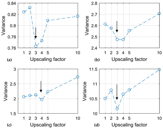
Figure 3.
(a) Variance against upscaling factor for blue band; (b) green band; (c) red band; and (d) near-infrared band using the simulated datasets. Optimum spatial resolution (OSR) is indicated with an arrow.
These findings are also compatible with the visual interpretation of the simulated figures, discussed earlier (Table 2), indicating that the pixel sizes 5 and 10 provide high mean-variance values for all bands, while the figures of pixel sizes 3 and 4 tend to give the sharpest contrast between the simulated buried target and the surrounding healthy vegetation.
The simulated results were further processed to estimate the optimal spatial resolution (OSR) for different vegetation indices. While several indices do exist in the relevant literature, as also indicated in [23], in this study, we focused only on three vegetation indices which are widely used for detection of archaeological proxies. These indices have been examined for all upscaling factors and include the Simple Ratio (SR), the Atmospheric Resistance Vegetation Index (ARVI), and the Normalized Difference Vegetation Index (NDVI). The equations of these indices are provided below:
whereas is the reflectance value at the near-infrared band, is the reflectance value at the red band, and is the reflectance value at the blue band.
The aggregated results of the SR, ARVI, and NDVI indices can be found in Figure 4, Figure 5 and Figure 6, respectively. In comparison with the spectral bands of Table 2, it is evident that all vegetation indices tend to provide a higher contrast of the simulated buried archaeological feature in comparison with the surrounding vegetation. This is valid for all upscaling factor values. However, similar observations to the one reported in the spectral bands can also be stated here: lower resolution scales (namely pixel sizes 5 and 10) tend to saturate the boundaries of the buried feature, while higher spatial resolutions (pixel sizes 2 and 3) tend to give a more evident outline border of the buried feature. From all vegetation indices, the SR (Figure 4) gives the sharpest outline at all pixel resolutions in comparison to the other indices. The statistical analysis of the OSR for SR (Figure 7a), ARVI (Figure 7b), and NDVI (Figure 7c) index is shown below. The OSR is indicated with an arrow in the graphs (Figure 7). As noticed, the optimum spatial resolution varies according to the vegetation product: for SR and ARVI highest spatial resolution products are required (pixel size 3) for better spectral discrimination of the buried feature, while for the NDVI index the OSR is set at factor 4. Once again, these findings from the statistical analysis are consistent with the visual interpretation findings from the Figure 4, Figure 5 and Figure 6.
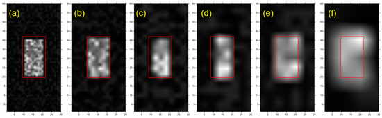
Figure 4.
(a) Simulated simple ratio (SR) datasets pixel size 1; (b) simulated SR datasets pixel size 2; (c) simulated SR datasets pixel size 3; (d) simulated SR datasets pixel size 4; (e) simulated SR datasets pixel size 5; and (f) simulated SR datasets pixel size 10.

Figure 5.
(a) Simulated Atmospheric Resistance Vegetation Index (ARVI) datasets pixel size 1; (b) simulated ARVI datasets pixel size 2; (c) simulated ARVI datasets pixel size 3; (d) simulated ARVI datasets pixel size 4; (e) simulated ARVI datasets pixel size 5; and (f) simulated ARVI datasets pixel size 10.
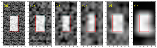
Figure 6.
(a) Simulated NDVI datasets pixel size 1; (b) simulated NDVI datasets pixel size 2; (c) simulated NDVI datasets pixel size 3; (d) simulated NDVI datasets pixel size 4; (e) simulated NDVI datasets pixel size 5; and (f) simulated NDVI datasets pixel size 10.
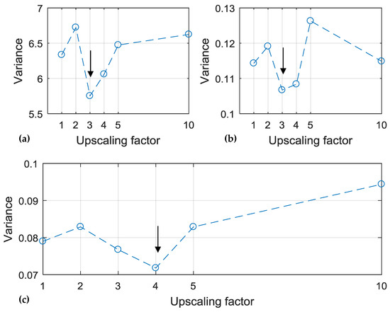
Figure 7.
(a) Variance against upscaling factor for Simple Ratio (SR) index; (b) Atmospheric Resistance Vegetation Index (ARVI); and (c) Normalized Difference Vegetation Index (NDVI), using the simulated datasets. Optimum spatial resolution (OSR) is indicated with an arrow.
3.2. WorldView-2 Image Analysis—Case Study 2
Following the simulation analysis of the ground spectroradiometric datasets, this section presents the results from the archaeological site of “Nea Paphos” in Cyprus (case study 2), which consists of an area with mixed spectral targets. Figure 8 presents the various pixel resolutions that are discussed in this section. Figure 8a displays the archaeological site of “Nea Paphos” at a spatial resolution of 2 m using the WorldView-2 NIR-R-G pseudo color composite; Figure 8b shows the same area resampled at a pixel size of 3 m; Figure 8c shows the area aggregated at a pixel size of 4 m; Figure 8d shows the upscaled resample area at a pixel size of 5 m; Figure 8e shows the archaeological site at a pixel size of 10 m, while Figure 8f shows the area resampled at a pixel size of 15 m. Finally, Figure 8g shows the area at the lowest pixel resolution of 30 m. The upscaling process was based on the nearest-neighbor resampling method as a fast computational algorithm. The aggregation process as mentioned by [21] is preferred through the use of coarse resolution data since it reduces any spatial registration errors and sensor noises, as well as removes part of the center-bias produced by the sensor point spread function. The utility of the nearest neighboring approach to resampling the remote sensing imagery has been also reported in other studies [24,25].
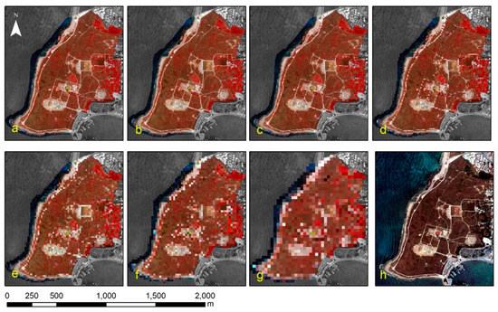
Figure 8.
(a) WorldView-2 Near Infrared-Red-Green (NIR-R-G) pseudo color composite of the archaeological site of “Nea Paphos” in Cyprus with a pixel size of 2 m; (b) resampled of (a) at a pixel size of 3 m; (c) resampled of (a) at a pixel size of 4 m; (d) resampled of (a) at a pixel size of 5 m; (e) resampled of (a) at a pixel size of 10 m; (f) resampled of (a) at a pixel size of 15 m; (g) resampled of (a) at a pixel size of 30 m; and (h) WorldView-2 R-G-B pseudo color composite of the site.
While no significant visual interpretation changes are evident between pixel resolution 3 m and 4 m, jagged edges can be observed at the next sampling level (pixel size 5 m), especially in the northern part of the archaeological site. The rest of the pixel resolutions images gradually add further jaggedness in the previously still images, while details of the archaeological site are no further visible at the lowest scale of observation (30 m) (Figure 8g).
As mentioned in the previous section, three regions of interests were selected for this case study (see also Figure 2 and Table 1). While the overall extent of these features is quite large, the archaeological proxies do not have a similar (spectral) pattern, since the features are disturbed and mixed up with other geographical entities of the area. Hence, the selection of the optimum spatial resolution (OSR) may vary for each observation target (ROI) according to the needs of each study.
An example of the interpretation detail at all pixel resolutions is given in the next figure. Figure 9a shows the original 2 m spatial resolution of the elliptical feature at the south part of the archaeological site (see Figure 2b, ROI-1), while Figure 9b–g presents the same feature in the various upscaling images. As is evident, the elliptical feature is apparent only in the resample pixel resolutions of 3 and 4 m (Figure 9b,c, respectively), while for the rest of the pixel sizes, the overall shape of the feature is mixed with its environment, thus making the interpretation difficult.
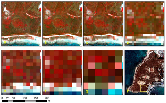
Figure 9.
(a) The elliptical shape observed at the southern part of the archaeological site of “Nea Paphos” with a pixel size of 2 m (see also Figure 2b); (b) the elliptical shape resampled of (a) at a pixel size of 3 m; (c) resampled of (a) at a pixel size of 4 m; (d) resampled of (a) at a pixel size of 5 m; (e) resampled of (a) at a pixel size of 10 m; (f) resampled of (a) at a pixel size of 15 m; (g) resampled of (a) at a pixel size of 30 m and (h) WorldView-2 R-G-B pseudo color composite of the site indicating the elliptical shape.
This finding is again consistent with the OSR statistical analysis of the mean-variance, presented in Figure 10. The OSR for ROI-1 (elliptical shape) is indicated with an arrow in all spectral bands. The OSR was estimated at the pixel resolution of 4 m spatial resolution. Beyond this pixel size, the mean-variance of the elliptical shape is increased for blue, green and red bands (visible part of the spectrum) and slightly increased for the near-infrared band. Similar findings were also reported for the rest of the areas under investigation (namely ROIs 2-3). In general, the curves of the mean-variance show a different trend for the different ROIs. This was expected since each region shares different properties and spectral behavior; however, a general tendency for all ROIs can be observed.
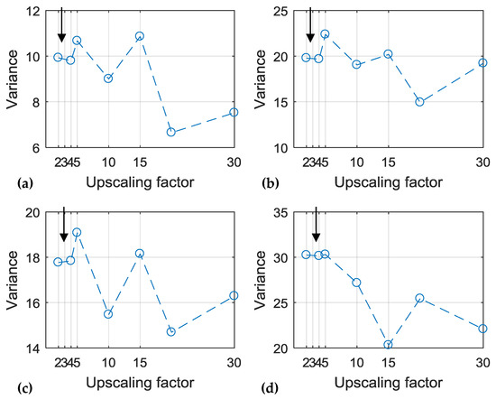
Figure 10.
(a) Variance against upscaling factor for blue band; (b) green band; (c) red band; and (d) near-infrared band over ROI-1 from the Nea Paphos archaeological site. Optimum spatial resolution (OSR) is indicated with an arrow.
The results of the mean-variance according to the upscaling factor for the rest of the regions of interest are shown in Figure 11 and Figure 12 (ROI-2, Figure 2c and ROI-3, Figure 2d), respectively. The OSR for the blue, green and red bands is calculated at 5 m spatial resolution for all ROIs, while for the near-infrared band the OSR is estimated to 10 m for ROI-2 and 4 m for ROI-3. The first threshold corresponds to the OSR where the vegetation proxy is homogenous, while beyond this pixel resolution (threshold), the vegetation proxy starts to be integrated in the rest of the environment.
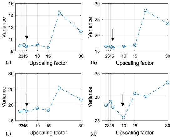
Figure 11.
(a) Variance against upscaling factor for blue band; (b) green band; (c) red band; and (d) near-infrared band over ROI-2 from the Nea Paphos archaeological site. Optimum spatial resolution (OSR) is indicated with an arrow.
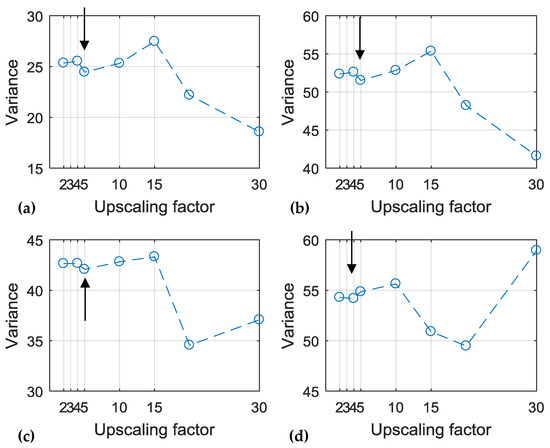
Figure 12.
(a) Variance against upscaling factor for blue band; (b) green band; (c) red band; and (d) near-infrared band over ROI-3 from the Nea Paphos archaeological site. Optimum spatial resolution (OSR) is indicated with an arrow.
The overall mean-variance diagram against the different upscaling factors demonstrates the general trend of the OSR for the archaeological site (Figure 13). It should be mentioned that the mean-variance was estimated using the local variance values of all three ROIs studied here, and not the total mean-variance of the entire archaeological site. As it was found the OSR for the blue and green band was estimated at 4 m spatial resolution (Figure 13a,b, respectively), and for the red, and near-infrared bands at 10 m (Figure 13c,d, respectively). Above these thresholds, the variance starts to increase, which is linked to the mixel (mixture element) phenomenon, that change the overall homogenous spectral signature of the ROIs. Indeed, beyond that pixel resolution, the features under investigations start to be integrated into their environment, thus giving heterogeneous spectral profiles and making the interpretation of the archaeological proxies difficult. Upon these findings, the OSR for all bands can be defined at a pixel resolution of 4 m.
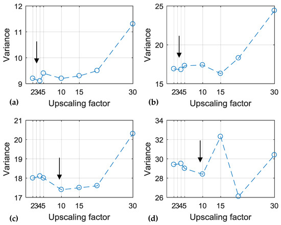
Figure 13.
(a) Mean-Variance against upscaling factor for blue band; (b) green band, (c) red band; and (d) near-infrared band over ROIs 1-3 from the Nea Paphos archaeological site. Optimum spatial resolution (OSR) is indicated with an arrow.
4. Discussion
From the previous results, some general comments can be raised here. Firstly, it is evident that the optimal resolution depends on the spatial properties of the targets under investigation, as this was also reported in the past [26]. As it was also reported in [23] optimal spatial resolution is primarily affected by the spatial and structural parameters of the targets. The spatial dimension of the features (archaeological proxies) under investigation is not the unique criterion for the selection of the optimal spatial resolution. This can be the case only in surveys where “pure” pixels are recorded in the remotely sensed sensors. In practice, the spectral confusion of the areas under investigation needs to be taken into consideration, as this has also been reported in other examples [21]. Indeed, the homogeneity of the area under investigation can be a critical aspect for the identification of the OSR [21]. The OSR as defined for the spectral bands is quite similar to other products derived from the same dataset, as in the case of the vegetation indices. As it was found in the case study 1, the OSR of the spectral bands was similar to the OSR of all three vegetation indices studied before.
In order to evaluate the final findings from the real experiment (case study 2), the OSR was further processed and interpreted in terms of detection and discrimination of archaeological proxies. For this reason, the WorldView-2 image of the archaeological site of “Nea Paphos” with a spatial resolution of 2 m was imported into a Geographical Information System (ArcMap v10.6) where further image enhancement techniques have been applied. The overall results, along with some considerations regarding the “differences” observed between the raw multispectral image (at 2 m spatial resolution), are presented below.
The first row of Figure 14 illustrates the area at the highest spatial resolution (2 m), while the OSR of 4 m is demonstrated at the next row (second row). The results are shown for the near-infrared part of the spectrum since this spectral region is the most sensitive for detecting archaeological proxies. In detail, Figure 14a,d refer to ROI-1 at a 2 m and 4 m spatial resolution, respectively, while, in a similar way, Figure 14b,e to ROI-2, and finally, Figure 14c,f to ROI-3.

Figure 14.
First row: WorldView-2 near-infrared band image at a spatial resolution of 2 m; second row: WorldView-2 near-infrared band image resampled at a spatial resolution of 4 m; (a) and (d) refer to ROI-1; (b) and (e) refer to ROI-2, and (c) and (f) refer to ROI-3). For the location of each ROI, refer to Figure 2.
As shown in Figure 14a,d both pixel resolutions (i.e., the original 2 m and the OSR 4 m resolution) visualize the outline of the elliptical shape (ROI-1). The highest spatial resolution (Figure 14a) provides as expected a much clearer representation. However, when it comes to observing the inner space of the elliptical feature, spectral confusion makes it difficult to set the boundaries of the elliptical shape at this high-resolution image. In contrary, the OSR image inner details of the archaeological proxies can be observed (Figure 14d, circled with yellow shape), since the local variance for this feature is minimized at this spatial resolution. Similar findings can also be observed for the linear feature (ancient road(?), ROI-2) at Figure 14b,e. Although the linear feature is visible in both pixel resolutions (original size 2 m and OSR at 4 m), the OSR minimizes the local variance along the feature, thus supporting visual interpretation. One of the finest examples of the suitability of the OSR regards the area at the western part of the site, namely the ROI-3. While 2 m spatial resolution (Figure 14c) partially shows some traces, the OSR image (Figure 14f) visualizes several small-size linear and semi-circular features, pointed with yellow arrows on the figure. This is an example where the high local variance of the highest spatial resolution creates a local spectral confusion at the area under investigation, while the OSR image provides a result with a low local spectral variance.
The profile of a linear transect over the elliptical shape at the southern part of the archaeological site (ROI-1) is given in the next figure (Figure 15). The location of the transect of a length of 90 m (45 pixels of 2 m resolution) is shown at the bottom right part of Figure 15. The profile is given for the “true” RGB composite (red-green-blue) at a pixel resolution of 2-m spatial resolution -indicated with continues lines, and at a pixel size of 4-m (OSR) with dashed lined. As demonstrated, for all bands of the resample image of 4 m, the spectral variance along the transect is smoother in comparison with the initial transect. Fluctuations of the spectral profile at the initial image (2 m) are becoming smaller in the degraded image. This “filtering” is not however changing the overall trend and shape of the spectral profile, for instance, the highest peaks and lowest values, which are still visible in the 4-m pixel size resolution image (as the one indicated for the green band with arrow).
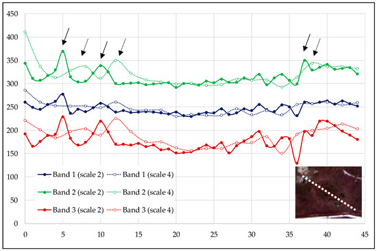
Figure 15.
Transect profile over the elliptical shape at the southern part of “Nea Paphos” (ROI-1, Figure 2b) as recorded for the red-green-blue bands at a pixel resolution of 2 and 4 m.
To further visual interpretation and spectral profiles of the horizontal transect, the OSR and the initial 2 m spatial resolution images were analyzed using four different quality image methods: (a) bias, (b) image entropy, (c) RASE (relative average spectral error), and (d) RMSE (root mean squared error). Bias metric is sensitive only to the difference in the mean values of the reference and the re-sampling image (i.e., OSR image) [20], while image entropy metric provides the information content of the image based on a probability distribution. Therefore, higher entropy values indicate a higher amount of information present in the OSR image. In contrast, the global spectral quality of the image can be evaluated using the RASE metric; lower values of RASE indicates better spectral quality [27]. Finally, RMSE metric estimates the difference of the variation between the reference (initial pixel size) and the OSR image. The OSR image is close to the reference image when the RMSE value is zero [28]. Their mathematical equations are listed below (Equations (4)–(7)), while more details regarding these methods can be found in [29,30].
The OSR of the “Nea Paphos” archaeological site of a pixel resolution of 4 m, was directly compared with the reference (initial) image of a resolution of 2 m. The process was performed in the MATLAB R2016b environment, using the Graphic Unit Interface (GUI) “Image Quality—Index Analysis GUI” accessible at [31,32]. Part of the results are demonstrated in Figure 16 and Figure 17. Figure 16 shows the results for the elliptical shape (ROI-1), while Figure 17 demonstrates the results from the linear feature of ROI-2. The first row (a) of Figure 16 and Figure 17 presents the results from the Bias method, while the second (b) and third (c) rows of Figure 16 and Figure 17 show the results of the RASE and RMSE methods, respectively. Column ii–v are related to the spectral bands of blue, green, red, and near-infrared, respectively. The first column (column i) indicates the RGB composite of the area at a 2 m and 4 m spatial resolution.
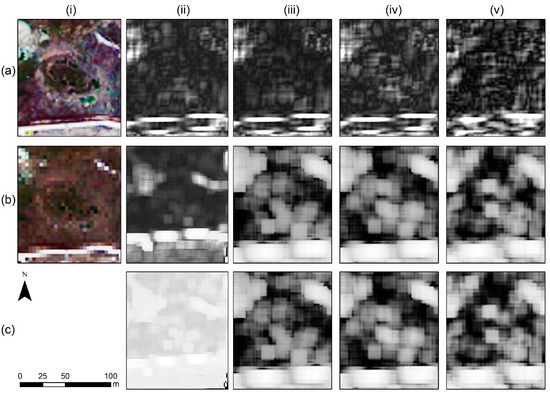
Figure 16.
Results after the image quality process for ROI-1 (elliptical shape) using the (a) bias, (b) RASE (relative average spectral error), and (c) RMSE (root mean squared error) methods. The first column (i) refers to pan sharpened and raw WorldView-2 image, while the second column (ii) refers to the results for the blue band and similarly the columns (iii), (iv) and (v) to the results of the green, red and near-infrared bands respectively.
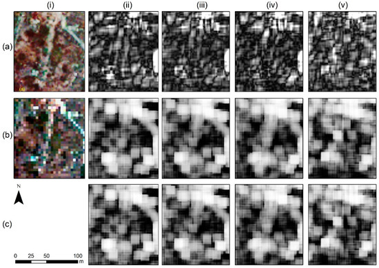
Figure 17.
Results after the image quality process for ROI-2 (linear feature) using the (a) bias, (b) RASE (relative average spectral error), and (c) RMSE (root mean squared error) methods. The first column (i) refers to pan sharpened and raw WorldView-2 image, while the second column (ii) refers to the results for the blue band and similarly the columns (iii), (iv) and (v) to the results of the green, red and near-infrared bands respectively.
As is evident in Figure 16 and Figure 17, the quality indices indicate similar results for the different spectral bands. The differences between the initial 2 m spatial resolution image and the degraded 4 m resolution do not follow the outlines of the edges of the elliptical shape (Figure 16) and the linear feature (Figure 17). The differences observed between the OSR image (4 m resolution) and the initial image (2 m resolution) do not affect the visual interpretation of the archaeological proxy per se but, rather, the whole area of the image, as an expected outcome of the degradation process of the datasets. So, the visual interpretation of the OSR image and the 2 m resolution image is not distorted in the archaeological proxy’s area only but, rather, follow a uniform difference between the reference and the resampled image.
The overall results from this quantitative analysis (i.e., comparison of the 2 m and the 4 m spatial resolution images) are indicated in Table 3. The table summarizes the comparison results for each quality image method (bias, entropy, RASE, and RMSE) for the different spectral bands. The comparison was made using the whole area of the archaeological site of “Nea Paphos”. Values close to zero (0) indicate identical images, with no significant spectral difference between the initial image and the OSR image. In general, the results are quite similar for all spectral bands, for each method used, while the best results are found on the blue band, which provide the lowest values. The overall low values from the Bias and Entropy method (close to 0) show that the degraded image of 4 m (OSR) has similar spectral context as the raw 2 m spatial resolution image, indicating that no significant spectral information was lost through the degradation process of the image. The low-value scores of the Entropy metric indicate that the information of the OSR image at 4 m pixel resolution remains almost the same as the one of the initial 2 m resolution image, despite the difference in the pixel size.
Table 3.
Quantitative analysis of original 2 m spatial resolution image against the OSR image (4 m).
5. Conclusions
Spatial resolution is a critical characteristic of satellite-based investigations used for archaeological prospections. This study aimed to make an introduction of the importance of the image resolution, following examples from the existing literature, and then analyze the spatial resolution of images in terms of defining the optimum observation scale for supporting archaeological prospection surveys, especially in areas with high spectral heterogeneity. For this reason, a high-resolution WorldView-2 image was used, and then systematically upscaled, while calculating the mean-variance of the regions of interest. The overall results indicate that higher spatial resolution is not always the optimum scale of observation, especially in areas with high spectral heterogeneity. The examples of the elliptical shape and the small linear and semi-circular feature of the archaeological site (Figure 14a,d,c,f, respectively) are some of the best examples of this argument. Quality analysis carried out between the raw image (2 m spatial resolution) and the OSR image (4 m spatial resolution) also indicates high image relevance. Thus, the aggregate image does not skip essential details (edges) from the initial dataset. Instead, it smooths the spectral profile, as shown in Figure 15, and better supports visual interpretation.
While in our case studies in this paper, the spatial extent and size of the archaeological proxies are a-priori known, in practice this is now always so straightforward. Indeed, the spatial resolution of buried archaeological features is usually unknown prior to the satellite investigation, which, however, can be retrieved from the existing archaeological knowledge and interpretation of the archaeological evidence. This kind of analysis can be used so as to set the spatial properties of the potential archaeological proxies, while other existing visible sites of the area under investigation and archive prospection datasets can be used as a guideline for the satellite investigation. We should, therefore, stress the point that archaeological prospection, in various forms, either from the ground or from space, should always be driven from archaeological evidence and archaeological queries which set the proper context for these technologies.
The choice of a simple degradation upscaling process, like the one implemented in our study, was based on similar considerations raised by [25]. When the scope of the study is not to simulate all conditions involved in remotely sensed data acquisition but to investigate the impact of a sampling system on the measurement of geographical entities, a simple model (such as those of nearest neighbor) can be used, assuming all other variables negligible. Of course, more sophisticated simulating upscaling methods do exist in the literature. Complex simulation models which include biophysical and atmospheric radiative transfer models can be found in [33], while spatial autocorrelation and semivariograms methods have been implemented by [34]. Other researchers have developed and utilized empirical statistical measures that express a relation between observed variance and spatial resolution. More details regarding such statistical measures for the optimal spatial resolution can be found in [35].
The overall findings of the current study are consistent with other similar studies working in different—non-archaeological—environments. As [20] stated in their study, there is no single-pixel size which would give the best interpretation result for all cases. Instead, there is an optimal pixel size of its own for each case study.
However, as [35] argued, choosing a spatial resolution for a remote sensing investigation may be a complex task if the area of interest contains a variety of targets with different land covers. Whereas new satellite sensors, as well as other unmanned aerial vehicle (UAVs), can provide today sub-meter and centimeter analysis products, the definition of the OSR is of critical importance when it comes to large projects which require systematic measurements and regular flight observations. Future studies will further aim to investigate the impact of both spectral and spatial resolution towards the detection of archaeological proxies, expanding the study to other indices, as well as other parameters studied here, such as the orientation of the subsurface remains.
Funding
The results are part of the project “Synergistic Use of Optical and Radar data for cultural heritage applications”, (PLACES), with grant number CULTURE/AWARD-YR/0418/0007 funded by the Republic of Cyprus.
Acknowledgments
The author would like to acknowledge the “CUT Open Access Author Fund” for covering the open access publication fees of the paper.
Conflicts of Interest
The author declares no conflict of interest.
References
- Luo, L.; Wang, X.; Guo, H.; Lasaponara, R.; Zong, X.; Masini, N.; Wang, G.; Shi, P.; Khatteli, H.; Chen, F.; et al. Airborne and spaceborne remote sensing for archaeological and cultural heritage applications: A review of the century (1907–2017). Remote Sens. Environ. 2019, 232, 111280. [Google Scholar] [CrossRef]
- Agapiou, A.; Lysandrou, V. Remote Sensing Archaeology: Tracking and mapping evolution in scientific literature from 1999–2015. J. Archaeol. Sci. Rep. 2015, 4, 192–200. [Google Scholar] [CrossRef]
- Ricchetti, E. Application of optical high resolution satellite imagery for archaeological prospection over Hierapolis (Turkey). In Proceedings of the 2004 IEEE International Geoscience and Remote Sensing Symposium (IGARSS 2004), Anchorage, AK, USA, 20–24 September 2004; Volume 6, pp. 3898–3901. [Google Scholar] [CrossRef]
- Barone, P.M.; Scardozzi, G. Optical high-resolution satellite imagery for the study of the ancient quarries of Hierapolis. In Ancient Quarries and Building Sites in Asia Minor. Research on Hierapolis in Phrygia and Other Cities in South-Western Anatolia: Archaeology, Archaeometry, Conservation; Ismaelli, T., Scardozzi, G., Eds.; Edipuglia: Bari, Italy, 2016; pp. 657–668. [Google Scholar]
- Aqdus, S.A.; Hanson, W.S.; Drummond, J. The potential of hyperspectral and multi-spectral imagery to enhance archaeological cropmark detection: A comparative study. J. Archaeol. Sci. 2012, 39, 1915–1924. [Google Scholar] [CrossRef]
- Calleja, F.J.; Pagés, R.O.; Díaz-Álvarez, N.; Peón, J.; Gutiérrez, N.; Martín-Hernández, E.; Cebada Relea, A.; Melendi, R.D.; Álvarez, F.P. Detection of buried archaeological remains with the combined use of satellite multispectral data and UAV data. Int. J. Appl. Earth Obs. Geoinf. 2018, 73, 555–573. [Google Scholar] [CrossRef]
- Lasaponara, R.; Masini, N. Detection of archaeological crop marks by using satellite Quick Bird multispectral imagery. J. Archaeol. Sci. 2007, 34, 214–221. [Google Scholar] [CrossRef]
- Agapiou, A.; Lysandrou, V.; Lasaponara, R.; Masini, N.; Hadjimitsis, D.G. Study of the Variations of Archaeological Marks at Neolithic Site of Lucera, Italy Using High-Resolution Multispectral Datasets. Remote Sens. 2016, 8, 723. [Google Scholar] [CrossRef]
- Sarris, A.; Papadopoulos, N.; Agapiou, A.; Salvi, M.C.; Hadjimitsis, D.G.; Parkinson, A.; Yerkes, R.W.; Gyucha, A.; Duffy, R.P. Integration of geophysical surveys, ground hyperspectral measurements, aerial and satellite imagery for archaeological prospection of prehistoric sites: The case study of Vészto-Mágor Tell, Hungary. J. Archaeol. Sci. 2013, 40, 1454–1470. [Google Scholar] [CrossRef]
- Traviglia, A.; Cottica, D. Remote sensing applications and archaeological research in the Northern Lagoon of Venice: The case of the lost settlement of Constanciacus. J. Archaeol. Sci. 2011, 38, 2040–2050. [Google Scholar] [CrossRef]
- Cerra, D.; Agapiou, A.; Cavalli, R.M.; Sarris, A. An Objective Assessment of Hyperspectral Indicators for the Detection of Buried Archaeological Relics. Remote Sens. 2018, 10, 500. [Google Scholar] [CrossRef]
- De Laet, V.; Paulissen, E.; Waelkens, M. Methods for the extraction of archaeological features from very high-resolution Ikonos-2 remote sensing imagery, Hisar (Southwest Turkey). J. Archaeol. Sci. 2007, 34, 830–841. [Google Scholar] [CrossRef]
- Orengo, H.A.; Petrie, C.A. Large-Scale, Multi-Temporal Remote Sensing of Palaeo-River Networks: A Case Study from Northwest India and its Implications for the Indus Civilisation. Remote Sens. 2017, 9, 735. [Google Scholar] [CrossRef]
- Agapiou, A.; Hadjimitsis, D.G.; Alexakis, D.D.; Papadavid, G. Examining the Phenological Cycle of Barley (Hordeum vulgare) Using Satellite and in situ Spectroradiometer Measurements for the Detection of Buried Archaeological Remains. Gisci. Remote Sens. 2012, 49, 854–872. [Google Scholar] [CrossRef]
- Winton, H.; Horne, P. National archives for National Survey Programmes: NMP and the English Heritage Aerial Photograph Collection. In Landscapes Through the Lens: Aerial Photographs and the Historic Environment, 1st ed.; Cowley, D.C., Standring, R., Abicht, M., Eds.; Aerial Archaeology Research Group: Oxbow, UK, 2010; Volume 1, pp. 7–18. ISBN 1842179810. [Google Scholar]
- Gojda, M.; Hejcman, M. Cropmarks in main field crops enable the identification of a wide spectrum of buried features on archaeological sites in Central Europe. J. Archaeol. Sci. 2012, 39, 1655–1664. [Google Scholar] [CrossRef]
- Aqdus, S.A.; Hanson, W.S.; Drummond, J. A Comparative Study for Finding Archaeological Crop Marks Using Airborne Hyperspectral, Multispectral and Digital Photographic Data. In Proceedings of the 2007 Annual Conference of the Remote Sensing and Photogrammetry Society, Newcastle, UK, 12–17 September 2007; pp. 177–182. [Google Scholar]
- D’Orazio, T.; Palumbo, F.; Guaragnella, C. Archaeological trace extraction by a local directional active contour approach. Patt. Recognit. 2012, 45, 3427–3438. [Google Scholar] [CrossRef]
- Agapiou, A.; Hadjimitsis, D.G.; Sarris, A.; Georgopoulos, A.; Alexakis, D.D. Optimum Temporal and Spectral Window for Monitoring Crop Marks over Archaeological Remains in the Mediterranean region. J. Archaeol. Sci. 2013, 40, 1479–1492. [Google Scholar] [CrossRef]
- Marceau, D.J.; Hay, G.J. Remote Sensing Contributions to the Scale Issue. Can. J. Remote Sens. 1999, 25, 357–366. [Google Scholar] [CrossRef]
- Tran, T.-B.; Puissant, A.; Badariotti, D.; Weber, C. Optimizing Spatial Resolution of Imagery for Urban Form Detection—The Cases of France and Vietnam. Remote Sens. 2011, 3, 2128–2147. [Google Scholar] [CrossRef]
- Agapiou, A. Enhancement of Archaeological Proxies at Non-Homogenous Environments in Remotely Sensed Imagery. Sustainability 2019, 11, 3339. [Google Scholar] [CrossRef]
- Agapiou, A.; Hadjimitsis, D.G.; Alexakis, D.D. Evaluation of Broadband and Narrowband Vegetation Indices for the Identification of Archaeological Crop Marks. Remote Sens. 2012, 4, 3892–3919. [Google Scholar] [CrossRef]
- Hasituya, C.Z.; Wang, L.; Liu, J. Selecting Appropriate Spatial Scale for Mapping Plastic-Mulched Farmland with Satellite Remote Sensing Imagery. Remote Sens. 2017, 9, 265. [Google Scholar] [CrossRef]
- Marceau, D.J.; Gratton, D.J.; Fournier, R.A.; Fortin, J.P. Remote sensing and the measurement of geographical entities in a forested environment. 2. The optimal spatial resolution. Remote Sens. Environ. 1994, 49, 105–117. [Google Scholar] [CrossRef]
- Nijland, W.; Addink, E.A.; De Jong, S.M.; Van der Meer, F.D. Optimizing spatial image support for quantitative mapping of natural vegetation. Remote Sens. Environ. 2009, 113, 771–780. [Google Scholar] [CrossRef]
- Johnson, B. Effects of Pansharpening on Vegetation Indices. ISPRS Int. J. Geo-Inf. 2014, 3, 507–522. [Google Scholar] [CrossRef]
- Jinju, J.; Santhi, N.; Ramar, K.; Sathya Bama, B. Spatial frequency discrete wavelet transform image fusion technique for remote sensing applications. Eng. Sci. Technol. Int. J. 2019, 22, 715–726. [Google Scholar] [CrossRef]
- Jagalingam, P.; Vittal Hegde, A. A Review of Quality Metrics for Fused Image. Aquat. Procedia 2015, 4, 133–142. [Google Scholar] [CrossRef]
- Ghassemian, H. A review of remote sensing image fusion methods. Inf. Fusion 2016, 32 Pt A, 75–89. [Google Scholar] [CrossRef]
- Vaiopoulos, A.D. Developing Matlab scripts for image analysis and quality assessment. In Proceedings of the SPIE 8181, Earth Resources and Environmental Remote Sensing/GIS Applications II, 81810B, Prague, Czech Republic, 26 October 2011. [Google Scholar] [CrossRef]
- Image Quality—Index Analysis GUI. Available online: https://www.mathworks.com/matlabcentral/fileexchange/41464-image-quality-index-analysis-gui (accessed on 3 December 2019).
- Verhoef, W.; Bach, H. Simulation of hyperspectral and directional radiance images using coupled biophysical and atmospheric radiative transfer models. Remote Sens. Environ. 2003, 87, 23–41. [Google Scholar] [CrossRef]
- Hyppänen, H. Spatial autocorrelation and optimal spatial resolution of optical remote sensing data in boreal forest environment. Int. J. Remote Sens. 1996, 17, 3441–3452. [Google Scholar] [CrossRef]
- Atkinson, M.P.; Aplin, P. Spatial variation in land cover and choice of spatial resolution for remote sensing. Int. J. Remote Sens. 2004, 25, 3687–3702. [Google Scholar] [CrossRef]


© 2020 by the author. Licensee MDPI, Basel, Switzerland. This article is an open access article distributed under the terms and conditions of the Creative Commons Attribution (CC BY) license (http://creativecommons.org/licenses/by/4.0/).