Topology-Aware Road Network Extraction via Multi-Supervised Generative Adversarial Networks

Abstract

Road network extraction from remote sensing images has played an important role in various areas. However, due to complex imaging conditions and terrain factors, such as occlusion and shades, it is very challenging to extract road networks with complete topology structures. In this paper, we propose a learning-based road network extraction framework via a Multi-supervised Generative Adversarial Network (MsGAN), which is jointly trained by the spectral and topology features of the road network. Such a design makes the network capable of learning how to “guess” the aberrant road cases, which is caused by occlusion and shadow, based on the relationship between the road region and centerline; thus, it is able to provide a road network with integrated topology. Additionally, we also present a sample quality measurement to efficiently generate a large number of training samples with a little human interaction. Through the experiments on images from various satellites and the comprehensive comparisons to state-of-the-art approaches on the public datasets, it is demonstrated that the proposed method is able to provide high-quality results, especially for the completeness of the road network.

1. Introduction

Road network extraction is a fundamental issue in remote sensing image processing, which can provide an important reference for road planning or surveys, or prior knowledge for the detection and recognition of vehicles, buildings, or other objects.

Most of the rule-based approaches rely on spectral behavior or intensity contrast [1], thus relying heavily on appropriate features to describe the “potential road regions” [2,3]. However, this kind of method may be limited in two ways [4]: Firstly, the spectral behaviors of the roads from various satellites can be very different. Secondly, it is hard to recognize aberrant road regions caused by occlusion or shadows in the remote sensing images. To address these limitations, recent works [3,5,6,7] have tried to reconstruct the road topology via multi-stage schemes according to “assistant information”, such as simple interaction [5], a 3D road surface model [6], pre-defined classifiers [7], or an aperiodic directional structure measurement [3,8]. However, such rule-based expert systems can easily fall into a difficult problem—that is, to cover all expected types of roads, they have to exhaustively establish the complex discriminate criterion and at last make it infeasible to tune such expert systems by hand. Thus, this calls for a machine learning approach.

To avoid the ad hoc trait of the feature-based methods, learning-based approaches have appeared over the past few decades. Based on the neural network, several works attempt to predict whether a given pixel is on the road [9,10]. In recent years, the development of deep neural networks [11] has provided a new solution for road network extraction. Learning-based methods, such as the higher-order CRF model [12], multi-level networks [1], or cascaded end-to-end convolutional neural networks [13] with various structures have been employed to find road regions from satellite images. Most of these learning-based approaches focus on the spectral behavior of the road regions, while a few of them take the topology of the road network into account, thus leading to the discontinuous road network map caused by the aberrant road regions, such as shadows and occlusion, as shown in the highlighted region of Figure 1.

Based on these considerations, we propose a topology-aware road network extraction framework via a Multi-supervised Generative Adversarial Network (MsGAN). The major contribution of the proposed network relies on a multi-supervised structure, where the generator is jointly trained by the road region map and the centerline map, so as to capture both the spectral and topology information of the road network. Such a scheme makes the network capable of learning how to “guess” the aberrant road cases based on the relationship between the road region and centerline; thus, it is able to provide a road network with integrated topology. On the other hand, to address the expensive labor-consuming problem of training sample production, we also propose a sample quality measurement so as to efficiently generate a large number of training samples with just a little human interaction. In the experiments, we present comprehensive comparisons to demonstrate the performance of the proposed MsGAN.

2. Related Work

Road network extraction is a long-standing problem in remote sensing image processing. According to previous surveys [4,14,15,16,17,18] and the latest works on road extraction [5,7], road network extraction can be roughly divided into three methods: rule-based, topology-based, and learning-based.

Early road extraction studies have preferred extracting roads by utilizing their visual or geometric features. Assuming that road regions often appear as thin, low-curvature, high-contrast structures, various filters and road segmentation connection methods (such as morphological filters [19], Gibbs point [20], directional filters [21], Kalman filters [22], line segments matching [23], and line primitive connection [24,25,26,27]) were proposed. To further improve extraction performance, more elaborate methods followed. Poullis and You, 2010 [28], employed Gabor filtering and tensor voting for geospatial feature inference classification. Then, followed by orientation-based segmentation, road centerlines were extracted to describe the road network. Inspired by this work, Grote et al., 2012 [29] extracted road networks by integrating the radiometric and geometric features of road regions. Then, by constructing a subgraph, potential road segments were connected to form the results. Based on the definition of pixel-wise polygonal areas, Hu et al., 2007 [30] and Zhang et al., 2011 [31] employed a pixel footprint detector to extract road regions. However, these methods are able to handle long and continuous road regions, which often failed for the cases of occlusion and shadows.

To address this problem, recent approaches have focused on the topology reconstruction of the road regions. With the observation that low-level road extraction methods are fragmented, Steger et al., 1998 [32], 1997 [33] first proposed constructing a road network topology according to the graph theory. Also benefiting from graph representation, Peteri and Ranchin, 2006 [34] developed a road shape extraction scheme by defining the active contours. Followed by these works, Ünsalan et al., 2012 [5] proposed a graph-based topology analysis scheme to refine the road map, in which spectral, shape, and gradient features are combined to generate approximate road primitives. By employing different road detection methods and introducing 3D road information, Ziems et al., 2012 [6] proposed a multi-model fusing scheme to combine the results of different models, which is able to present impressive robustness and detection performance. Based on a pre-trained spectral-spatial classifier, Shi et al., 2015 [7] developed a road centerline extraction scheme, which significantly improves the detection robustness. To suppress the interference of the undesired textures and overcome the blur effect of feature descriptor mathematical morphology (MM), general adaptive neighborhood (GAN)-based MM (GANMM) [35] was applied to form the morphological profiles. Zang et al., 2016 [8] proposed an aperiodic directional structure measurement for road structure description, where such a measurement considers not only the geometry features, but also includes an aperiodicity measurement term to evaluate the “low social conformity” of potential road regions, meaning that it is thus able to provide spectral character and contrast-independent road extraction results.

However, in order to reconstruct complete road network topology, most recent studies have tended to adopt increasingly complex multi-stage or multi-model schemes. As pointed out by Mnih et al., 2010 [1], such an ad hoc manner may introduce extra parameters or computational burden, thus leading to the reduction of the robustness and speed of the whole system.

On the other hand, learning-based approaches attempt to predict whether a given pixel is a road or not, according to the context around the target pixel [9,10,36,37,38,39,40]. The extraction is similar to the task of salient objects extraction or segmentation [41,42,43,44,45,46,47]. Liu et al., 2017 [46] exploited multiscale and multilevel information to extract edges and boundaries, which is also adopted by us as the multilevel discriminator. By observing that the pixels near road boundaries have large responses, while the pixels within the roads have small responses to the Laplacian of Gaussian filter, Yuan et al., 2011 [48] extracted roads automatically by clustering the well-aligned pixels according to a proposed locally excitatory globally inhibitory oscillator network (LEGION). Recently, the development of a deep neural network [11] has provided a new idea for road network extraction. Mnih and Hinton, 2010 [1] first proposed a multi-level network, which aims to assign each pixel a label to denote whether it belongs to a road region or not. Wegner et al., 2013 [12] proposed a higher-order CRF model for road labeling, in which the road likelihood is amplified for thin chains of super-pixels. Cheng et al., 2017 [13] proposed a cascaded end-to-end convolutional neural network (CasNet) to address the road segmentation and centerline extraction tasks, where such an approach works well for urban roads with explicit spectral features. Most of these learning-based approaches focus on the spectral behavior of the road regions, while few of them take the topology of the road network into account, thus leading to a discontinuous road network map caused by shadow and occlusion.

3. Method

To acquire the large amount of training samples, we first used an automatic sample production method to generate training sets, which contains both of the road centerline and region maps, with just a little human interaction. With the created samples, the MsGAN was proposed to generate road centerlines directly. In the following subsections, we will describe the architecture and loss functions of the proposed network in detail.

3.1. Automatic Sample Production

Manual labeling is the most accurate method for creating a training sample, but it is very labor-consuming to acquire. In this section, we will introduce our solution to efficiently produce a large number of training samples with only a little human interaction.

Specifically, since we do not have any road network information, previous methods such as [3,5,6] can be applied for the initial centerline estimation (in this paper, the system proposed by Zang et al., 2016 [3] is employed). In this approach, the applied training patches have the size of $1024\times 1024$ pixels, and we tended to select training samples with consistent local structures. According to this criterion, a confidence evaluation algorithm was designed to help in the selection of the most appropriate regions for the selection of suitable training samples. As shown in Figure 2, the better samples should be selected in the long and straight road region, as highlighted in the zoomed-in patch on the right, while the area of ambiguity should be avoided (as shown in the zoomed-in patch on the left).

Therefore, our idea was to give a score for each sample candidate (with a size of $1024\times 1024$), which were generated by using a sliding window over the whole image with a step of 256 pixels. Then, a set of small patches were created along the road centerlines for each sample candidate. Specifically, the size of the local patches was $64\times 64$ with a step of 20 pixels. Then, the sample candidates with smaller scores (calculated as average scores of the local patches) with high probability were selected as training samples. Suppose there are N local patches in a sample candidate. The score of the candidate $S_c$ can be calculated as:

$$S_c=\frac{1}{N}\sum _{k=1}^N{s}_k$$

(1)

where $s_k$ represents the measurement of each local patch, which can be calculated by the following scheme.

Given the extracted road centerline L, for each road pixel $p\in L$, $A_p$ denotes the set of road pixels in the local area centered at p. Then, our aim was to find a target straight line $l_t:y=ax+b$, such that the sum of the distance from $p_i\in A_p$ to $l_t$ is at a minimum. Formally, our aim can be written as:

$$s_k=arg\underset{a,b}{min}\frac{1}{n}(\sum _{i=1}^n\frac{{(a{x}_i-y_i+b)}^2}{a^2+1});$$

(2)

where $(x_i,y_i)$ is the position of pixel $p_i$, and n is the size of $A_p$.

To solve this problem, ${\displaystyle \sum _{i=1}^n}\frac{{(a{x}_i-y_i+b)}^2}{a^2+1}$ can be denoted as $F(a,b)$, and it is then easy to get $b=\overline{y}-a\overline{x}$ ($\overline{x}=\frac{1}{n}{\displaystyle \sum _{i=1}^n}{x}_i$ and $\overline{y}=\frac{1}{n}{\displaystyle \sum _{i=1}^n}{y}_i$). Then we have:

$$F(a,b)=\frac{M{a}^2+Na+T}{a^2+1}$$

(3)

where

$$\begin{array}{cc}\hfill M& =\sum x_i^2-\frac{1}{n}{(\sum x_i)}^2\hfill \\ \hfill N& =\frac{2}{n}\sum x_i\sum y_i-2\sum x_i{y}_i\hfill \\ \hfill T& =\sum y_i^2-\frac{1}{n}{(\sum y_i)}^2\hfill \end{array}$$

(4)

Then, after the transposition of terms, we have $(M-F(a,b))a^2+Na+T-F(a,b)=0$. To guarantee Equation (3) has a solution, we have:

$$N^2-4(M-F(a,b))(T-F(a,b))\ge 0.$$

(5)

It is

$$-4F{(a,b)}^2+4(M+T)F(a,b)+N^2-4MT\ge 0.$$

(6)

Notice that the above equation must have one or two intersections with a straight line $y=0$ (since $N^2-4MT+{(M+T)}^2=N^2+{(M-T)}^2\ge 0$), where denoting the solutions as $s_1,s_2$, and the smaller one, say $s_1\le s_2$, would be the desired value of $F(a,b)$. Then, by solving the equation $(M-F(a,b))a^2+Na+T-F(a,b)=0$, we have $a=(-N\pm \sqrt{N^2-4(M-s_1)(T-s_1)})/2(M-s_1)$, since $\sqrt{N^2-4(M-s_1)(T-s_1)}=0$; thus we have an analytical solution to this problem $a=-\frac{N}{M-s_1}$.

Then, for a selected sample candidate, a set of three maps, including the original image, the region map, and the centerline map were created to form the training set. Here, the road centerline map was generated with the help of a previous work [3], and the region map was generated by [7].

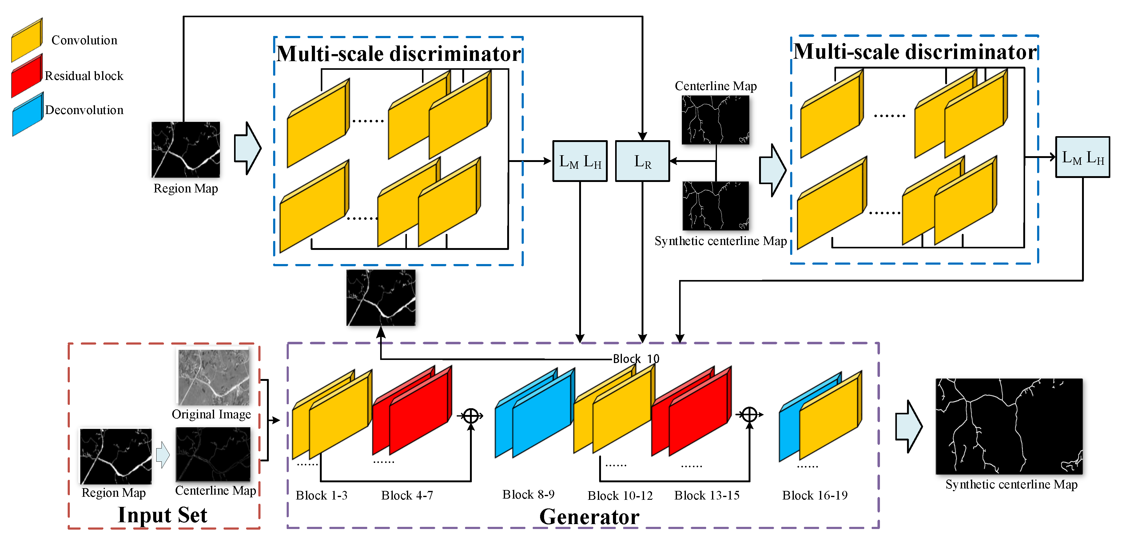
3.2. Network Architecture

By reviewing previous learning-based road extraction works, we found that most of the methods focused mainly on the spectral and spatial performance of road regions, while few of them paid attention to the topological completeness of road networks.

To address this issue, inspired by the generative adversarial networks (GAN) [49], this paper proposes MsGAN, a topology-aware road centerline generation network via a multi-supervised manner. Specifically, two multi-scale discriminators are employed in the proposed network, where one of them takes the region map as the supervisor while the other one takes the centerline map as the supervisor. In this structure, the first part of the network emphasizes the detection of road regions, and the other one focuses mainly on the road topology reconstruction.

The architecture of the MsGAN is shown in Figure 3, which consists of two discriminators and a generator. A set of three images, including the original image, the region map, and the centerline map are employed to train the network. Then, for the generator G, it is composed of two parts. Firstly, the original image is fed into the first part, made up of four residual blocks [50], four convolutional layers, and two deconvolutional layers. Each residual block comprises two convolutional layers, two InstanceNorm [51] layers, and one ReLU layer. The output of the first part (the 9th block) is the generated road region map.

Similarly to the first part, the second is comprised of four residual blocks, three convolutional layers, and two deconvolutional layers. In addition, we add two skipped connections to both parts, similar to the structure of U-Net [52], considering that the added skipped connection can decrease the loss of enlargement and preserve more detail. The output of the second part (the 10th block) is the generated road region map; the output of the second part (the 19th block) is the generated road centerline map.

For the discriminators, the first one was trained by the road region map to make the network aware of the spectral structures, and another one trained by the centerline map considering the topological connectivity of road networks in order to instruct the extraction. In each discriminator, there are four identical sub-discriminators, including five convolutional layers, which takes the same image with four scales as inputs, respectively, thus making the network capable of extracting roads of different widths.

In general, the output of the discriminator is 1 or 0, while we assume the image as a Markov random field consisting of N pixel patches, beyond which the pixels are independent, and we set the size N as 70. A smaller value of N implies the fewer required parameters, thus resulting in less running time and making it appropriate for more images with various sizes; however, this also leads to weak anti-noise capability. Additionally, we also added the pre-trained VGG network as the other part of MsGAN, where the feature maps of eight layers were extracted respectively from real and fake inputs.

3.3. Loss Function

As mentioned above, our goal was to extract road centerlines from the satellite or aerial images. We used the generative adversarial training scheme: the generator aims to produce as accurate centerlines as possible, while the two discriminators are trained to distinguish the fake road region maps and centerline maps. For our task, the loss function contains four parts: the multi-supervised loss, the hierarchical per-pixel loss, the perceptual loss, and the region loss.

To extract the roads with different widths, in each discriminator, four identical sub-discriminators with four-scale inputs were combined together. The multi-supervised loss is as follows:

$$L_M(G,D_k)=\sum _{k=1}^4{L}_{su{b}_D}(G,D_k).$$

(7)

where $D_k\left(x\right)$ is the k-th sub-discriminator, and $L_{su{b}_D}$ denotes the conditional adversarial loss for the sub-discriminators, which can be written as:

$$L_{su{b}_D}(G,D)=E_{x,y\in P_{data}(x,y)}\left[logD(x,y)\right]+E_{x\in P_{data}\left(x\right)}\left[log(1-D(x,G\left(x\right)))\right].$$

(8)

Here, x and y represent the input and ground truth, respectively; $G\left(x\right)$ represents the output of the generator; and $D\left(x\right)$ represents the output of the discriminator. $P_{data}\left(x\right)$ represents the distribution of data.

Meanwhile, considering how the output of the discriminator may miss low feature distinctions, we added an adversarial loss called hierarchical per-pixel loss, whose aim was to collect the feature differences from all layers under L1 norms:

$$L_H(G,D_k)=\sum _{i=1}^4\sum _{k=1}^{N_i}\frac{1}{N_i}{\Vert D_k\left(G\left(x\right)\right)-D_k\left(y\right)\Vert }_1.$$

(9)

where $N_i$ is the layer number of the i-th sub-discriminator.

For the generator, we took in the perceptual loss as the recent super-resolution task [53], which has been proven effective:

$$L_P\left(G\right)=\sum _{k=i_1}^{i_N}{\lambda }_k{P}_k(G\left(x\right),y),$$

(10)

and $P_k(G\left(x\right),y)$ is defined as:

$$P_k(G\left(x\right),y)={\Vert H_k\left(G\left(x\right)\right)-H_k\left(y\right)\Vert }_1$$

(11)

where $H_k$ denotes the pre-trained VGG [54], $P_k$ denotes the difference of the k-th layer, ${\lambda }_k$ is the weight of the k-th layer, and $i_1\sim i_N$ means the N-extracted layers.

In addition, the road region image was taken as an extra supervisor, and a designed region loss was employed to punish the generated centerlines out of the area, which can be written as the following formula:

$$L_R\left(G\right)=\sum _{P\in P_R}{{\Vert G\left(x\right)}_R-y_R\Vert }_1+{\lambda }_R\sum _{P^{\prime }\in \overline{P_R}}{{\Vert G\left(x\right)}_{R^{\prime }}-y_{R^{\prime }}\Vert }_1$$

(12)

where ${\lambda }_R$ is the weight for punishing the outliers; $R_p$ denotes the pixels within the road region; and $\overline{R_p}$ denotes the pixels out of the road region.

The total objective function contains the four parts: $L_M$, $L_H$, $L_G$, $L_R$. We tried to minimize $T^{*}$ for the generator and maximize $T^{*}$ for the discriminators. The final objective function is as follows:

$$T^{*}=arg\underset{G}{min}\underset{D}{max}{L}_{total}$$

(13)

$$L_{total}=L_M+L_H+L_G+L_R$$

(14)

4. Results and Analysis

Implementation details. Our approach was based on a PyTorch framework on a PC with one Titan X GPU. The network was trained from scratch using an Adam solver [55], and the learning rate was 0.0004. Weights were initialized from a Gaussian distribution with mean $\mu =0$ and standard deviation $\sigma =0.02$. For the generator, the activation layer was ReLU, while for the discriminator the activation layer was LeakyReLU with a slope of $0.2$. The number of layers in the perceptual loss branch was eight layers extracted from VGG. The weights of the four middle layers were $\frac{1}{32}$, the next two were $\frac{1}{16}$, and the last two were $\frac{1}{4}$ and $\frac{1}{2}$, respectively. ${\lambda }_R$ was set as 20 to punish the error out of road regions.

Quantitative measurements. The widely used quantitative measurements, recall, precision, and F1 score were employed to evaluate the overall detection performance. Specifically, they can be written as:

$$\begin{array}{c}\hfill recall\left(R\right)=\frac{TP}{TP+FN}\\ \hfill precision\left(P\right)=\frac{TP}{TP+FP}\\ \hfill \mathrm{F}1\mathrm{score}\left(F\right)=\frac{2·precision·recall}{precision+recall}\end{array}$$

(15)

where $TP$, $FN$, and $FP$ stand for true-positive, false-negative, and false-positive, respectively.

Datasets. To comprehensively evaluate the performance of our approach, several groups of experiments were designed on various datasets. Firstly, based on the remote sensing images of the Pleiades-1A satellite and a public dataset released by Cheng et al., 2017 [13], we provided some intuitional results to show how the network parameters and structure could affect the road extraction results. Meanwhile, we also compared our method with the single-supervised GAN (i.e., the SsGAN, which is trained only by the road centerline map), to demonstrate the effect of the extra supervisor on various datasets.

Then, images from various satellite sensors, including Geoeye, QuickBird, Pleiades-1A, and GaoFen2, were applied to evaluate the performance of our approach, where various terrains like urban, rural, and mountain were involved and the ground truth was manually created.

Finally, our approach was compared with some of the latest learning-based approaches on two public datasets released by Cheng et al., 2017 [13] and Mnih, 2013 [56]. We also evaluated our method on the Pleiades-1A remote sensing images, which covered an entire city of China (Shaoshan City in Hunan province), in which the reference was obtained by the ground survey and provided by the China Transportation & Telecommunication Center, and presented a comparison with the latest rule-based road network extraction methods.

4.1. Evaluation of the Network Performance

In this section, we first discuss the setting of parameters and present how different parameters affected the results. Then, we make a comparison against the centerline generation strategy of road region extraction plus the post-processing route to demonstrate the superiority of the MsGAN. Finally, we also make a comparison against the single-supervised GAN (SsGAN), which is trained by just the centerline map, to demonstrate the advantage of the multi-supervisor.

Evaluation of the network parameters. For the proposed MsGAN, the number of sub-discriminators affects the extraction results. Due to the image resolution and the various widths of roads, the characteristics of road regions can be very different over different sources or even in the same image, thus making it challenging to capture the roads with different scales. To address this issue, the multi-scale [46,57] discriminator is employed, but the number of sub-discriminators should be set to balance the efficiency and extraction performance. In this experiment, results of different numbers of sub-discriminators are collected, as shown in Figure 4 (Column (c) to (f) is the number of sub-discriminators from two to five). It can be viewed that, as the number of sub-discriminators increases, more roads are able to be detected, thus leading to more complete topological structures. As the number increases to four or five, the results tend to be convergent. Therefore, considering the efficiency and performance, the number of sub-discriminators was set as four for all experiments.

Comparison to the post-processing-based centerline generation scheme. The proposed MsGAN aimed to generate the road region and centerline map via one network. Here, we set up an experiment to compare with the segmentation-thinning manner, which was to obtain the road region map first and then get the road centerline map through the post-processing scheme, such as thinning or the image skeleton extraction algorithm. The segmentation-thinning manner has been widely used by previous rule-based approaches to create road centerlines, which may result in inaccurate or pseudo-extraction results, while MsGAN is able to directly extract complete road centerlines. Specifically, we designed a comparison with the network of removing the supervision of centerline maps and corresponding losses. Then, after obtaining the road region map, a thinning method was applied to generate the final centerline maps. Here, following previous procedures, Gaussian filtering was applied before the thinning process to generate a more complete road network.

The results are shown in Figure 5 (column (a) and (b) are the input images and ground truth; column (c) is the result of the MsGAN; column (d) and (e) are the road region map and corresponding thinning centerline result). It can be viewed that, despite the adding of Gaussian filtering, the gaps or pseudo-lines can still be observed due to the two-step operation (as highlighted in the red box), while MsGAN can produce more complete centerline results directly.

Evaluation of the extra supervisor. Then, to demonstrate the effect of the extra supervisor, the proposed MsGAN was compared to the single-supervised GAN, that is, SsGAN. In this experiment, we just removed the supervision of road region maps and corresponding losses, while keeping other parts of the network unchanged. The training and testing phase was based on a public dataset released by Cheng et al., 2017 [13]. For the SsGAN, the training sample consisted of an original image and a labeled road centerline image. Corresponding results are shown in Figure 6 (column (a) and (b) are the input images and ground truth, (c) and (d) are the results of SsGAN and MsGAN). The corresponding quantitative statistics of the MsGAN and SsGAN on this dataset are shown in

Table 1. Quantitative statistics on images in Figure 6 and dataset [13]. Images 1 to 3 are from top to bottom.

	Image 1			Image 2			Image 3			Avg.(test set)
$\mathit{\rho }=\mathbf{2}$	R	P	F	R	P	F	R	P	F	R	P	F
SsGAN	0.922	0.962	0.942	0.955	0.971	0.963	0.901	0.962	0.930	0.926	0.965	0.945
MsGAN	0.952	0.988	0.970	0.963	0.978	0.971	0.944	0.962	0.953	0.960	0.975	0.967

.

It can be seen that the result of SsGAN suffers some gaps when the road topology is complex or the spectral performance of the road region is not visually significant. However, for the proposed MsGAN, due to the network that is desired to achieve not only the road region detection, but also the road topology reconstruction, it is thus able to produce a road network with complete topology, as highlighted in the red box.

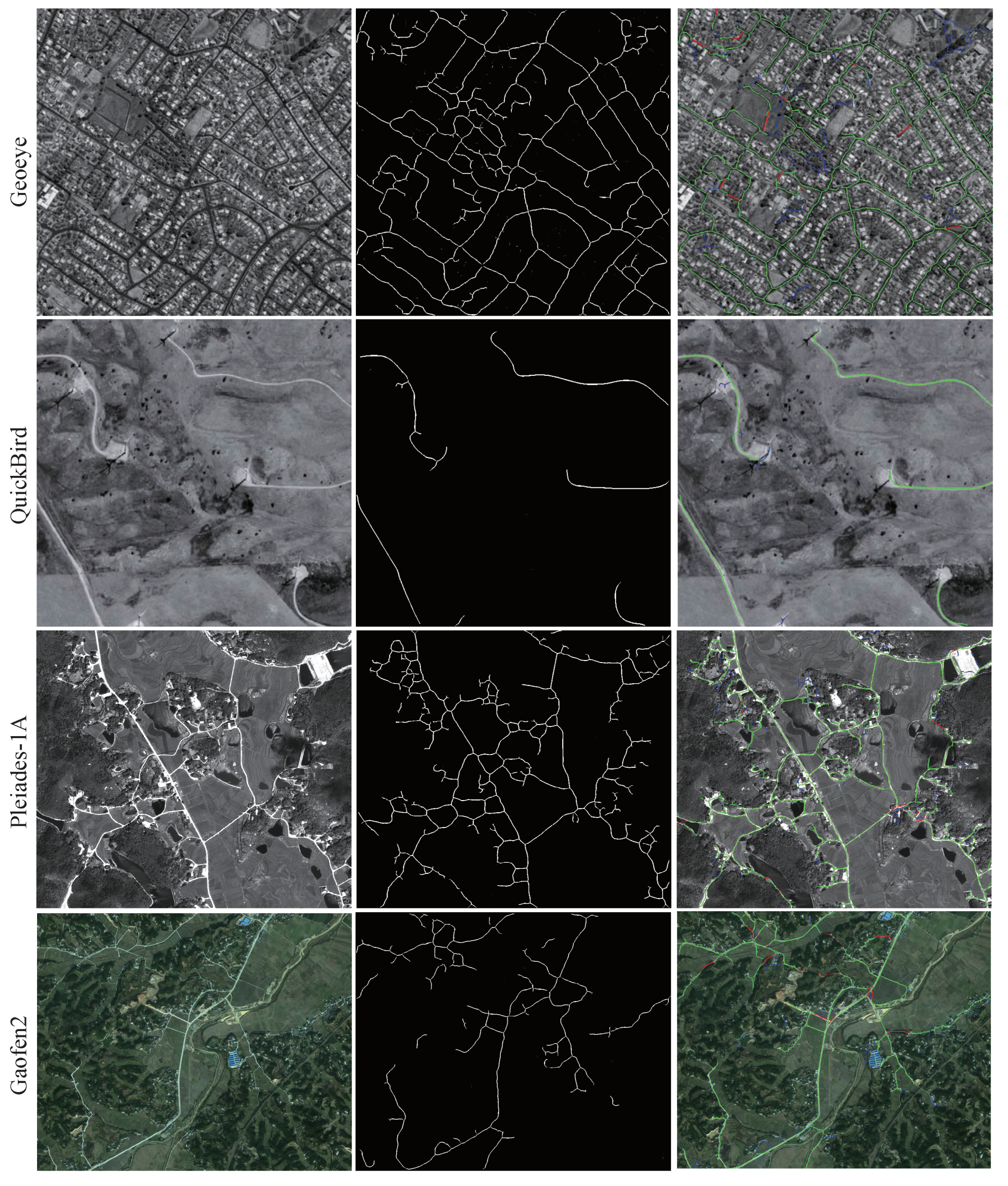
4.2. Evaluation on Various Datasets

In this section, we evaluate the proposed approach on images from four different sensors, including Geoeye, QuickBird, Pleiades-1A, and GaoFen2 satellites, where the resolutions of these images are 0.5 m, 0.5 m, 0.5 m, and 1 m, respectively, and the ground truth data were manually generated.

Test on Geoeye satellite image. The proposed approach has been tested on ten selected Geoeye images (including seven city region images, two rural region images, and one mountain region image, and most of them are about $1000\times 1000$ patches) with 13,627,789 pixels. Figure 7 shows an example which was also applied in a previous work [5], as shown in the Figure 7. Where column (b) is the extracted centerline result of our approach, column (c) is the comparison to the ground truth, where the green, blue, and red lines represent the true-positive, false-positive, and false-negative detections. From the results, it can be observed that despite how there are many interferences, such as buildings or occlusions, our approach has received pretty high recall, and the overall detection quality is quite satisfactory. The average quantitative measurements over ten images are listed in the second row of

Table 2. Quantitative statistics on images from various sensors.

Data	Recall	Precision	F1 Score
Geoeye	0.888	0.841	0.864
QuickBird	0.861	0.855	0.858
Pleiades-1A	0.857	0.862	0.860
GaoFen2	0.881	0.833	0.856

.

Test on QuickBird satellite image. Then, the proposed approach was tested on ten classic QuickBird images, including three mountain region images, three city region images, and four rural region images. Also, the sizes of these images are about $1000\times 1000$, and involves 10,516,297 pixels in total. The selected example, as shown in the Figure 7, was also tested in previous works [3,5]. The results of Unsalan et al., 2012 [5] did not perform well because the images were JPEG compressed, while for the result of Zang et al., 2016 [3], the terrain boundary was misidentified as being a road; hence, the precision was not satisfactory. For our result, since there was not much interference, the recall was able to achieve almost 90%, while the precision was also satisfied. The average quantitative measurements over ten images are listed in the third row of Table 2.

Test on Pleiades-1A satellite image. For this satellite, we tested the whole Shaoshan city. Details of such data can be viewed in Section 4.3. The selected example is a typical patch, as shown in Figure 7, in which various challenging cases for road network extraction are involved, such as the curved roads, shadows, and occlusions. From the extraction result, it can be viewed that most of these cases have been well-handled due to the topology learning. The average quantitative measurements over the whole Shaoshan City are listed in the fourth row of Table 2.

Test on GaoFen2 image. The proposed approach has also been tested on two GaoFen2 images with a size of $8000\times 8000$ and 7000 × 11,000 pixels. The selected example was chosen from the rural region, as shown in Figure 7. Some road-like structures, such as the rivers or boundaries of the farmland, can be observed. In previous works, like that by Zang et al., 2016 [3], these structures were likely to be falsely recognized. In our approach, such errors can be effectively eliminated due to the direct extraction of road centerlines. The average quantitative measurements are listed in the last row of Table 2.

4.3. Comparisons

In this section, the designing of two comparison groups is presented to demonstrate the performance of the proposed MsGAN. Specifically, two types of methods are employed for comparison: Firstly, we compare with some of the latest deep neural networks on two public datasets released by Cheng et al., 2017 [13] and Mnih, 2013 [56]; and secondly, we compare with some of the latest rule-based road extraction approaches on the images from Pleiades-1A which covers Shaoshan city in China.

Comparison with learning-based approaches. In this experiment, some learning-based approaches were applied for comparison. The dataset is public, and was released by Cheng et al., 2017 [13] which can be downloaded from the address http://www.escience.cn/people/guangliangcheng/Datasets.html. The dataset consists of 224 very high-resolution (VHR) images from Google Earth with a resolution of 1.2 m per pixel, and it is known to be the largest road dataset with accurate segmentation maps and centerline maps. The approaches applied for testing include those by Huang et al., 2009 [10], Miao et al., 2013 [58], Shi et al., 2015 [7], Cheng et al., 2016 [59], Baseline-Casnet [13], and Casnet [13], and we employed the same samples used in Cheng et al., 2017 [13] for the comparison. Results of previous works were provided by Cheng et al., 2017 [13], and corresponding results are shown in Figure 8.

Where column (a) is the input image; columns (b)–(h) are the results corresponding to the methods of Huang et al., Miao et al., Shi et al., Cheng et al., Baseline-Casnet, Casnet, and our approach; and column (i) is the ground truth. The results in the first to the third rows correspond to the three samples employed in [13], and the results in the fourth and fifth rows are the zoomed-in patch intercept from Image 3, as shown in the red and blue box. From the results, it can be seen that the performances of the latest road centerline extraction method proposed by Cheng et al., 2017 [13] and our approach are rather similar, while in the zoomed-in patch, our results have better local topology similarity to the ground truth, as highlighted in the green box.

For the quantitative measurement, following the buffer widths method proposed by Wessel et al., 2003 [60] and Cheng et al., 2017 [13], statistics of the above methods, along with our approach were collected under the parameter of $\rho =2$, and the results are shown in

Table 3. Quantitative statistics of different methods on the dataset [13].

	Image 1			Image 2			Image 3			Avg.(test set)
$\mathit{\rho }=\mathbf{2}$	R	P	F	R	P	F	R	P	F	R	P	F
Huang et al. [10]	0.975	0.814	0.887	0.964	0.722	0.826	0.967	0.747	0.843	0.959	0.738	0.834
Miao et al. [58]	0.930	0.816	0.882	0.885	0.705	0.784	0.894	0.724	0.800	0.896	0.718	0.797
Shi et al. [7]	0.938	0.920	0.925	0.940	0.920	0.930	0.864	0.849	0.856	0.893	0.907	0.900
Cheng et al. [59]	0.960	0.910	0.935	0.990	0.907	0.946	0.949	0.824	0.881	0.931	0.896	0.913
Casnet-baseline [13]	0.942	0.908	0.921	0.927	0.911	0.919	0.933	0.791	0.856	0.924	0.874	0.898
Casnet [13]	0.979	0.946	0.962	0.997	0.965	0.981	0.957	0.943	0.950	0.963	0.954	0.959
MsGAN	0.983	0.968	0.975	0.995	0.981	0.988	0.953	0.973	0.963	0.960	0.974	0.967

, and the best performance of each criterion are emphasized in boldface. As shown, our method has better performance in road centerline results than the other methods. In all of the three images, our method achieves the highest results in precision and the F1 score, as seen in Images 2 and 3; although we are slightly lower than Casnet in the recall, our overall performance is higher than the others.

For the second group of the experiment, the proposed approach, along with several latest networks, were evaluated on the Massachusetts Roads Dataset, which is public and was released by Mnih, 2013 [56]. In the comparison, the same patches applied in a previous work [61] are presented, and corresponding results are shown in Figure 9, where column (a) is the input image; columns (b)–(g) are the results corresponding to methods of Wegner et al., 2013 [12], Wegner et al., 2015 [62], Zhong et al., 2016 [63], Wei et al., 2017 [61], Cheng et al., 2017 [13] and our approach, respectively; and column (h) is the ground truth. The results of previous work by Wegner et al., 2013 [12], Wegner et al., 2015 [62], Zhong et al., 2016 [63], and Wei et al., 2017 [61] were provided by Wei et al., 2017 [61], and the results of Cheng et al., 2017 [13] were implemented with little changes to adapt to the dataset.

It is viewed that, for the challenging cases presented, the feature-based CRF scheme [12,62] did not perform well due to the interference of terrain or buildings, and the results either suffered from incomplete topology or heavy false alarm. Learning-based algorithms [13,61,63] have better performance. For the result of Zhong et al., 2016 [63], major road network topology structures have been captured, but errors often occurred around the buildings. The approaches of Wei et al., 2017 [61] and Cheng et al., 2017 [13] were derived from CNNs, which were able to produce high-quality extraction results. However, some “gaps” can still be observed at the road region with shadows or occlusion, and the fine structures cannot be identified, such as the roads marked with double lines. Our approach was able to provide the road network with more complete topology, as shown in column (g).

Corresponding statistics are shown in

Table 4. Quantitative statistics of different methods on the Massachusetts Dataset [56].

Method	Recall	Precision	F1 Score
Wegner et al. [12]	0.322	0.405	0.359
Wegner et al. [62]	0.679	0.471	0.556
Zhong et al. [63]	0.686	0.435	0.532
Wei et al. [61]	0.729	0.606	0.662
Cheng et al. [13]	0.783	0.812	0.797
MsGAN	0.871	0.853	0.862

. It can be seen that previous approaches by Wegner et al., 2013 [12], Wegner et al., 2015 [62], Zhong et al., 2016 [63], and Wei et al., 2017 [61] have unsatisfactory performance, where either the recall or the precision is lower than $0.75$. The approach of Cheng et al., 2017 [13] performs well for this dataset, and apparent improvement is observed for the overall F1 score. McGAN performed quite well, where the recall moved up more than 7 points, and there a 3 point improvement for the precision can also be observed.

Comparison with latest feature-based approaches. In this part, we evaluate our approach on the remote sensing image of Shaoshan City recorded by the Pleiades-1A satellite with a resolution 0.5 m. In the prediction phase, the whole image was divided into patches with a size of $1000\times 1000$. Then, the results of these patches were merged together according to the gradient change direction of the boundary pixels. Details can be viewed in [3].

Shaoshan is a typical mountainous city, covering 247 square kilometers in the mid-south region of China. The size of the whole satellite image is 28,648 × 37,929 pixels, in which various roads and terrains are involved. The whole image is divided into $1000\times 1000$ patches with 30% overlap. We evaluated our approach on each patch, and finally merged them together. The reference was acquired by the ground survey and provided by the China Transportation & Telecommunication Center.

Some typical results are shown in Figure 10, where the selected examples include typical terrains in the surrounding regions of Shaoshan city, such as the plain area, mountain area, town area, and so on. It can be observed that most of the errors occur in regions where the roads are occluded for a long distance, because the gaps may not be captured in this case. For the quantitative measurement, three recent rule-based road extraction methods [5,7,8] were applied for comparison. We also gathered the statistics of the result generated only by performing feature learning. The corresponding results are listed in

Table 5. Comparisons of recent rule-based road detection methods on Shaoshan City.

Method	R	P	F
Ünsalan et al., 2012 [5]	0.803	0.663	0.726
Shi et al., 2015 [7]	0.730	0.769	0.749
Zang et al., 2016 [8]	0.779	0.714	0.745
MsGAN	0.857	0.862	0.860

. From the results, it can be observed that the result of Unsalan et al., 2012 [5] had high recall, while the precision was not satisfied; Shi et al., 2015 [7] and Zang et al., 2016 [8] got more balanced results for recall and precision, and had a similar F1 score. The performance of the proposed MsGAN was beyond our expectations, where both the recall and precision had significantly improved, and the overall extraction quality increased by about 15 percentage points, compared with previous road extraction works.

5. Conclusions

In this paper, we presented a learning-based road network extraction scheme via a multi-supervised generative adversarial network (MsGAN). The motivation of this paper was to directly extract accuracy road centerlines with integrated topology. The contribution of this paper relied on a proposed multi-supervisor scheme to capture not only the spectral, but also the topology information of the road regions; thus, this makes the network capable of learning how to “guess” the aberrant road cases, which is caused by occlusion and shadow.

References

1. Mnih, V.; Hinton, G.E. Learning to Detect Roads in High-Resolution Aerial Images. In European Conference on Computer Vision; Springer: Berlin/Heidelberg, Germany, 2010; pp. 210–223. [Google Scholar]
2. Martin, D.R.; Fowlkes, C.C.; Malik, J. Learning to detect natural image boundaries using local brightness, color, and texture cues. IEEE Trans. Pattern Anal. Mach. Intell. 2004, 26, 530–549. [Google Scholar] [CrossRef]
3. Zang, Y.; Wang, C.; Cao, L.; Yu, Y.; Li, J. Road Network Extraction via Aperiodic Directional Structure Measurement. IEEE Trans. Geosci. Remote Sens. 2016, 54, 1–14. [Google Scholar] [CrossRef]
4. Baumgartner, A.; Steger, C.; Mayer, H.; Eckstein, W. Multi-Resolution, Semantic Objects, and Context for Road Extraction. In Semantic Modeling for the Acquisition of Topographic Information from Images and Maps; Birkhäuser: Basel, Switzerland, 1997; pp. 140–156. [Google Scholar]
5. Ünsalan, C.; Sirmacek, B. Road network detection using probabilistic and graph theoretical methods. IEEE Trans. Geosci. Remote Sens. 2012, 50, 4441–4453. [Google Scholar] [CrossRef]
6. Ziems, M.; Breitkopf, U.; Heipke, C.; Rottensteiner, F. Multiple-model based verification of road data. In Proceedings of the XXII ISPRS Congress, Melbourne, Australia, 25 August–1 September 2012; Volume I-3. [Google Scholar]
7. Shi, W.Z.; Miao, Z.L.; Debayle, J. An Integrated Method for Urban Main-Road Centerline Extraction From Optical Remotely Sensed Imagery. IEEE Trans. Geosci. Remote Sens. 2014, 52, 3359–3372. [Google Scholar] [CrossRef]
8. Zang, Y.; Wang, C.; Yu, Y.; Luo, L.; Yang, K.; Li, J. Joint Enhancing Filtering for Road Network Extraction. IEEE Trans. Geosci. Remote Sens. 2016, 99, 1–15. [Google Scholar] [CrossRef]
9. Mokhtarzade, M.; Zoej, M.J.V. Road detection from high-resolution satellite images using artificial neural networks. Int. J. Appl. Earth Obs. Geoinf. 2007, 9, 32–40. [Google Scholar] [CrossRef]
10. Huang, X.; Zhang, L. Road centreline extraction from high resolution imagery based on multiscale structural features and support vector machines. Int. J. Remote Sens. 2009, 30, 1977–1987. [Google Scholar] [CrossRef]
11. Hinton, G.E.; Salakhutdinov, R.R. Reducing the Dimensionality of Data with Neural Networks. Science 2006, 313, 504–507. [Google Scholar] [CrossRef] [PubMed]
12. Wegner, J.D.; Montoya-Zegarra, J.A.; Schindler, K. A Higher-Order CRF Model for Road Network Extraction. In Proceedings of the 2013 IEEE Conference on Computer Vision and Pattern Recognition, Portland, OR, USA, 23–28 June 2013; pp. 1698–1705. [Google Scholar]
13. Cheng, G.; Wang, Y.; Xu, S.; Wang, H.; Xiang, S.; Pan, C. Automatic Road Detection and Centerline Extraction via Cascaded End-to-End Convolutional Neural Network. IEEE Trans. Geosci. Remote Sens. 2017, 55, 3322–3337. [Google Scholar] [CrossRef]
14. Amo, M.; Martinez, F.; Torre, M. Road extraction from aerial images using a region competition algorithm. IEEE Trans. Image Process. 2006, 15, 1192–1201. [Google Scholar] [CrossRef]
15. Kong, H.; Audibert, J.Y.; Ponce, J. General road detection from a single image. IEEE Trans. Image Process. 2010, 19, 2211–2220. [Google Scholar] [CrossRef]
16. Mena, J.B. State of the art on automatic road extraction for GIS update: a novel classification. Pattern Recognit. Lett. 2003, 24, 3037–3058. [Google Scholar] [CrossRef]
17. Unsalan, C.; Boyer, K.L. A system to detect houses and residential street networks in multispectral satellite images. Comput. Vision Image Underst. 2005, 98, 423–461. [Google Scholar] [CrossRef]
18. Das, S.; Mirnalinee, T.T.; Varghese, K. Use of Salient Features for the Design of a Multistage Framework to Extract Roads From High-Resolution Multispectral Satellite Images. IEEE Trans. Geosci. Remote Sens. 2011, 49, 3906–3931. [Google Scholar] [CrossRef]
19. Katartzis, A.; Sahli, H.; Pizurica, V.; Cornelis, J. A model-based approach to the automatic extraction of linear features from airborne images. IEEE Trans. Geosci. Remote Sens. 2001, 39, 2073–2079. [Google Scholar] [CrossRef]
20. Stoica, R.; Descombes, X.; Zerubia, J. A Gibbs Point Process for Road Extraction from Remotely Sensed Images. Int. J. Comput. Vis. 2004, 57, 121–136. [Google Scholar] [CrossRef]
21. Gamba, P.; Dell’Acqua, F.; Lisini, G. Improving urban road extraction in high-resolution images exploiting directional filtering, perceptual grouping, and simple topological concepts. IEEE Geosci. Remote Sens. Lett. 2006, 3, 387–391. [Google Scholar] [CrossRef]
22. Movaghati, S.; Moghaddamjoo, A.; Tavakoli, A. Road Extraction From Satellite Images Using Particle Filtering and Extended Kalman Filtering. IEEE Trans. Geosci. Remote Sens. 2010, 48, 2807–2817. [Google Scholar] [CrossRef]
23. Shi, W.; Zhu, C. The line segment match method for extracting road network from high-resolution satellite images. IEEE Trans. Geosci. Remote Sens. 2002, 40, 511–514. [Google Scholar]
24. Yang, J.; Wang, R.S. Classified road detection from satellite images based on perceptual organization. Int. J. Remote Sens. 2007, 28, 4653–4669. [Google Scholar] [CrossRef]
25. Wiedemann, C.; Hinz, S. Automatic extraction and evaluation of road networks from satellite imagery. Int. Arch. Photogramm. Remote Sens. 1999, 32, 95–100. [Google Scholar]
26. Wiedeman, C.; Ebner, H. Automatic completion and evaluation of road networks. Int. Arch. Photogramm. Remote Sens. 2000, 33, 976–986. [Google Scholar]
27. Hinz, S.; Wiedemann, C. Increasing efficiency of road extraction by self-diagnosis. Photogramm. Eng. Remote Sens. 2004, 70, 1457–1466. [Google Scholar] [CrossRef]
28. Poullis, C.; You, S. Delineation and geometric modeling of road networks. ISPRS J. Photogramm. Remote Sens. 2010, 65, 165–181. [Google Scholar] [CrossRef]
29. Grote, A.; Heipke, C.; Rottensteiner, F. Road network extraction in suburban areas. Photogramm. Rec. 2012, 27, 8–28. [Google Scholar] [CrossRef]
30. Hu, J.; Razdan, A.; Femiani, J.C.; Cui, M.; Wonka, P. Road Network Extraction and Intersection Detection From Aerial Images by Tracking Road Footprints. Int. J. Remote Sens. 2007, 45, 4144–4157. [Google Scholar] [CrossRef]
31. Zhang, J.; Lin, X.; Liu, Z.; Shen, J. Semi-automatic road tracking by template matching and distance transformation in urban areas. IEEE Trans. Geosci. Remote Sens. 2011, 32, 8331–8347. [Google Scholar] [CrossRef]
32. Steger, C. An Unbiased Detector of Curvilinear Structures. IEEE Trans. Pattern Anal. Mach. Intell. 1998, 20, 113–125. [Google Scholar] [CrossRef]
33. Steger, C.; Mayer, H.; Radig, B. The role of grouping for road extraction. In Automatic Extraction of Man-Made Objects from Aerial and Space Images (II); Springer: Basel, Switzerland, 1997; pp. 245–256. [Google Scholar]
34. Peteri, R.; Ranchin, T. Automated road network extraction using collaborative linear and surface models. In Proceedings of the MAPPS/ASPRS 2006 Fall Conference “Measuring the Earth II: Latest Develoopments with Digital Surface Modelling and Automated Feature Extration”, San Antonio, TX, USA, 6–10 November 2006. [Google Scholar]
35. Debayle, J.; Pinoli, J.C. General Adaptive Neighborhood Image Processing: Part I: Introduction and Theoretical Aspects. J. Math. Imaging Vis. 2006, 25, 245–266. [Google Scholar] [CrossRef]
36. Qin, Y.; Chi, M.; Liu, X.; Zhang, Y.; Zeng, Y.; Zhao, Z. Classification of High Resolution Urban Remote Sensing Images Using Deep Networks by Integration of Social Media Photos. In Proceedings of the IGARSS 2018—2018 IEEE International Geoscience and Remote Sensing Symposium, Valencia, Spain, 22–27 July 2018; pp. 7243–7246. [Google Scholar]
37. Chi, M.; Sun, Z.; Qin, Y.; Shen, J.; Benediktsson, J.A. A novel methodology to label urban remote sensing images based on location-based social media photos. Proc. IEEE 2017, 105, 1926–1936. [Google Scholar] [CrossRef]
38. Zhou, J.; Yu, B.; Qin, J. Multi-level spatial analysis for change detection of urban vegetation at individual tree scale. Remote Sens. 2014, 6, 9086–9103. [Google Scholar] [CrossRef]
39. He, F.; Zhou, T.; Xiong, W.; Hasheminnasab, S.; Habib, A. Automated aerial triangulation for UAV-based mapping. Remote Sens. 2018, 10, 1952. [Google Scholar] [CrossRef]
40. Zhao, X.; Yu, B.; Liu, Y.; Chen, Z.; Li, Q.; Wang, C.; Wu, J. Estimation of Poverty Using Random Forest Regression with Multi-Source Data: A Case Study in Bangladesh. Remote Sens. 2019, 11, 375. [Google Scholar] [CrossRef]
41. Cheng, M.M.; Mitra, N.J.; Huang, X.; Torr, P.H.S.; Hu, S.M. Global Contrast based Salient Region Detection. IEEE Trans. Pattern Anal. Mach. Intell. 2015, 37, 569–582. [Google Scholar] [CrossRef] [PubMed]
42. Cheng, M.M.; Warrell, J.; Lin, W.Y.; Zheng, S.; Vineet, V.; Crook, N. Efficient salient region detection with soft image abstraction. In Proceedings of the IEEE International Conference on Computer Vision, Sydney, NSW, Australia, 1–8 December 2013; pp. 1529–1536. [Google Scholar]
43. Borji, A.; Cheng, M.M.; Hou, Q.; Jiang, H.; Li, J. Salient object detection: A survey. arXiv 2014, arXiv:1411.5878. [Google Scholar]
44. Borji, A.; Cheng, M.M.; Jiang, H.; Li, J. Salient Object Detection: A Benchmark. IEEE Trans. Image Process. 2015, 24, 5706–5722. [Google Scholar] [CrossRef]
45. Cheng, M.M.; Liu, Y.; Hou, Q.; Bian, J.; Torr, P.; Hu, S.M.; Tu, Z. HFS: Hierarchical feature selection for efficient image segmentation. In European Conference on Computer Vision; Springer: Cham, Switzerland, 2016; pp. 867–882. [Google Scholar]
46. Liu, Y.; Cheng, M.M.; Hu, X.; Wang, K.; Bai, X. Richer Convolutional Features for Edge Detection. In Proceedings of the IEEE Conference on Computer Vision and Pattern Recognition, Honolulu, HI, USA, 21–26 July 2017; pp. 3000–3009. [Google Scholar]
47. Chen, M.; Habib, A.; He, H.; Zhu, Q.; Zhang, W. Robust feature matching method for SAR and optical images by using Gaussian-gamma-shaped bi-windows-based descriptor and geometric constraint. Remote Sens. 2017, 9, 882. [Google Scholar] [CrossRef]
48. Yuan, J.; Wang, D.; Wu, B.; Yan, L.; Li, R. LEGION-Based Automatic Road Extraction From Satellite Imagery. IEEE Trans. Geosci. Remote Sens. 2011, 49, 4528–4538. [Google Scholar] [CrossRef]
49. Goodfellow, I.J.; Pouget-Abadie, J.; Mirza, M.; Xu, B.; Warde-Farley, D.; Ozair, S.; Courville, A.; Bengio, Y. Generative Adversarial Networks. Adv. Neural Inf. Process. Syst. 2014, 3, 2672–2680. [Google Scholar]
50. He, K.; Zhang, X.; Ren, S.; Sun, J. Deep residual learning for image recognition. In Proceedings of the IEEE Conference on Computer Vision and Pattern Recognition, Las Vegas, NV, USA, 27–30 June 2016; pp. 770–778. [Google Scholar]
51. Ulyanov, D.; Vedaldi, A.; Lempitsky, V. Instance Normalization: The Missing Ingredient for Fast Stylization. arXiv 2016, arXiv:1607.08022. [Google Scholar]
52. Ronneberger, O.; Fischer, P.; Brox, T. U-Net: Convolutional Networks for Biomedical Image Segmentation; Springer International Publishing: Cham, Switzerland, 2015; pp. 234–241. [Google Scholar]
53. Johnson, J.; Alahi, A.; Li, F.F. Perceptual Losses for Real-Time Style Transfer and Super-Resolution. In Proceedings of the European Conference on Computer Vision, Amsterdam, The Netherlands, 8–16 October 2016; pp. 694–711. [Google Scholar]
54. Simonyan, K.; Zisserman, A. Very Deep Convolutional Networks for Large-Scale Image Recognition. arXiv 2014, arXiv:1409.1556. [Google Scholar]
55. Kingma, D.P.; Ba, J. Adam: A Method for Stochastic Optimization. arXiv 2014, arXiv:1412.6980. [Google Scholar]
56. Mnih, V. Machine Learning for Aerial Image Labeling. Ph.D. Thesis, University of Toronto, Toronto, ON, Canada, 2013. [Google Scholar]
57. Wang, T.C.; Liu, M.Y.; Zhu, J.Y.; Tao, A.; Kautz, J.; Catanzaro, B. High-resolution image synthesis and semantic manipulation with conditional gans. In Proceedings of the IEEE Conference on Computer Vision and Pattern Recognition, Salt Lake City, UT, USA, 18–23 June 2018; pp. 8798–8807. [Google Scholar]
58. Miao, Z.; Shi, W.; Zhang, H.; Wang, X. Road centerline extraction from high-resolution imagery based on shape features and multivariate adaptive regression splines. IEEE IEEE Geosci. Remote Sens. Lett. 2013, 10, 583–587. [Google Scholar] [CrossRef]
59. Cheng, G.; Zhu, F.; Xiang, S.; Wang, Y.; Pan, C. Accurate urban road centerline extraction from VHR imagery via multiscale segmentation and tensor voting. Neurocomputing 2016, 205, 407–420. [Google Scholar] [CrossRef]
60. Wessel, B.; Wiedemann, C. Analysis of automatic road extraction results from airborne SAR imagery. Appl. Therm. Eng. 2003, 71, 276–290. [Google Scholar]
61. Wei, Y.; Wang, Z.; Xu, M. Road Structure Refined CNN for Road Extraction in Aerial Image. IEEE Geosci. Remote Sens. Lett. 2017, 14, 709–713. [Google Scholar] [CrossRef]
62. Wegner, J.D.; Montoya-Zegarra, J.A.; Schindler, K. Road networks as collections of minimum cost paths. ISPRS J. Photogramm. Remote Sens. 2015, 108, 128–137. [Google Scholar] [CrossRef]
63. Zhong, Z.; Li, J.; Cui, W.; Jiang, H. Fully convolutional networks for building and road extraction: Preliminary results. In Proceedings of the 2016 IEEE International Geoscience and Remote Sensing Symposium (IGARSS), Beijing, China, 10–15 July 2016; pp. 1591–1594. [Google Scholar]
Figure 1. Challenges of road network extraction from remote sensing image.
Remotesensing 11 01017 g001
Figure 2. The automatic sample production.
Remotesensing 11 01017 g002
Figure 3. Architecture of the proposed MsGAN.
Remotesensing 11 01017 g003
Figure 4. Results of different parameter settings. (a) shows the original images; (b) is the ground truth; (c) is the output of MsGAN with two discriminators; (d) is three discriminators; (e) is four discriminators; (f) is five discriminators.
Remotesensing 11 01017 g004
Figure 5. Comparison with the segmentation-thinning centerline extraction scheme. (a) shows the original images; (b) is the ground truth; (c) is the output of MsGAN; (d) is the output of MsGAN aiming to produce road region maps; (e) is the thinning results of the produced road region maps.
Remotesensing 11 01017 g005
Figure 6. Comparison with SsGAN on the dataset released by Cheng et al., 2017 [13]. (a) shows the original images; (b) is the ground truth; (c) is the result of MsGAN; (d) is the result of SsGAN.
Remotesensing 11 01017 g006
Figure 7. Our road extraction results on various sensors.
Remotesensing 11 01017 g007
Figure 8. Comparisons with latest methods on dataset [13] (the results of previous works provided by Cheng et al., 2017 [13]). (a) Original image; (b) result of Huang et al., 2009 [10]; (c) result of Miao et al., 2013 [58]; (d) result of Shi et al., 2015 [7]; (e) result of Cheng et al., 2016 [59]; (f) result of Baseline-Casnet [13]; (g) result of Casnet [13]; (h) result of MsGAN; (i) result of the reference map.
Remotesensing 11 01017 g008
Figure 9. Comparison with the latest state-of-the-art methods on the dataset [56] (the results of previous works were provided by Wei et al., 2017 [61]). (a) Original image; (b) result of Wegner et al., 2013 [12]; (c) result of Wegner et al., 2015 [62]; (d) result of Zhong et al., 2016 [63]; (e) result of Wei et al., 2017 [61]; (f) result of Cheng et al., 2017 [13]; (g) result of MsGAN; (h) ground truth.
Remotesensing 11 01017 g009
Figure 10. Typical results of Pleiades-1A satellite image on Shaoshan city.
Remotesensing 11 01017 g010