Abstract
Lineament mapping, which is an important part of any structural geological investigation, is made more efficient and easier by the availability of optical as well as radar remote sensing data, such as Landsat and Sentinel with medium and high spatial resolutions. However, the results from these multi-resolution data vary due to their difference in spatial resolution and sensitivity to soil occupation. The accuracy and quality of extracted lineaments depend strongly on the spatial resolution of the imagery. Therefore, the aim of this study was to compare the optical Landsat-8, Sentinel-2A, and radar Sentinel-1A satellite data for automatic lineament extraction. The framework of automatic approach includes defining the optimal parameters for automatic lineament extraction with a combination of edge detection and line-linking algorithms and determining suitable bands from optical data suited for lineament mapping in the study area. For the result validation, the extracted lineaments are compared against the manually obtained lineaments through the application of directional filtering and edge enhancement as well as to the lineaments digitized from the existing geological maps of the study area. In addition, a digital elevation model (DEM) has been utilized for an accuracy assessment followed by the field verification. The obtained results show that the best correlation between automatically extracted lineaments, manual interpretation, and the preexisting lineament map is achieved from the radar Sentinel-1A images. The tests indicate that the radar data used in this study, with 5872 and 5865 lineaments extracted from VH and VV polarizations respectively, is more efficient for structural lineament mapping than the Landsat-8 and Sentinel-2A optical imagery, from which 2338 and 4745 lineaments were extracted respectively.
1. Introduction
The mapping of the linear structural segments, which are called “lineaments”, on the Earth’s surface has always been an important part of any structural geological investigation. Lineaments reveal the architecture of the underlying rocks, which formed as a result of various tectonic (deformational) processes throughout the geological history of a region [1]. Structural geological investigations, alongside lithological mapping, collectively called geological mapping, are the basis for the prospection, exploration, and mining of various mineral deposits. Structural studies of the geological units surrounding mineral deposits is an important task toward understanding the genesis and accommodation of similar mineral resources because the identification of important structural events and their time in ore districts allows the construction of genetic models for ore formation. Moreover, the structural geology of a region is also important in understanding the geological history of a region, which is, in turn, vital for modeling various paleoclimatic and paleogeographic processes in the past [2]. Because of being hard and time-consuming, conventional ground-based mapping techniques are not efficient for structural geological studies of many mountainous regions, including the Pamir plateau studied here. Therefore, it is necessary to develop automatic, less time-consuming approaches for geological mapping of such regions, using satellite images and computing software and algorithms that would help and guide field observations.
From previous studies, one can conclude that lineaments usually occur as edges with tonal differences in satellite images and that most of the detection approaches are based on edge enhancement and filtering techniques [3,4,5]. These studies proposed two principal techniques for lineament identification and extraction from remotely sensed data. The first technique implies the enhancement and visual interpretation of linear structural segments using image enhancement techniques, namely image ratioing, image fusion, and directional and edge-detection filters, after which a lineament vector map can be produced using manual digitizing techniques [6,7,8]. Although efficient, this technique is quite time-consuming and requires the user to digitize lineaments manually. On the other hand, the second technique allows the detection and automatic extraction of the linear segments using computer software and algorithms, finally producing a lineament map [9,10,11]. Linear feature extraction, in the automatic approach, involves both manual visualization and automatic lineament extraction with the use of such software as PCI GeoAnalyst, Geomatica, Canny algorithm [12], and Matlab [13]. The application of filters (directional, Laplacian, Sobel, and Prewitt kernels) on particular bands or RGB combinations have been explored in different regions using air photographs and satellite images for lineament detection and the interpretation by numerous studies [14,15,16,17,18,19]. The most widely used software for the automatic lineament extraction is the LINE module of the PCI Geomatica [20]. The manual and automated methods of lineament extraction both can give reliable results. The manual method has been widely used for the validation of the lineaments extracted by automated technique [21]. However, the manual interpretation of the enhanced images for extracting the structural information can be a difficult task, time-consuming, and highly dependent on the quality of the analysis and expert experience [22]. Consequently, with the increase of computing power and the development of more advanced computer algorithms, automatic lineament extraction techniques have become widely used in the last few decades.
Recently, the development and progress in geographic information systems (GIS) and remote sensing allowed for the exploitation of a variety of data sources and techniques in the characterization of lineaments. Therefore, remote sensing data from both optical and radar sensors have been widely used in lineament mapping. The spatial resolution of remotely sensed imagery plays an important role in the quality of produced lineament maps. Investigators [20] compared Landsat ETM+ and ASTER in the quality of the extracted lineaments and concluded that the higher the spatial resolution, the higher the quality of the lineament maps. Thus, data fusion with a radar or the use of synthetic-aperture radar (SAR) images and, similarly, image fusion with Landsat band-8 (panchromatic) or the use of Landsat band-8 improved the number of lineaments extracted in further studies [21,23]. Shaded relief models are also widely used and considered as a powerful tool for lineament enhancement in topographic data [24]. These models owe this advantage to the artificial solar illumination and inclination angles that can vary and help in the identification of lineaments in a range of orientations by recognizing the shadowing effects, which produce boundaries between light and dark tones [25]. The shadowing effects are generated by abrupt changes in the elevation that reflects linear features on the surface of the Earth. The illumination angle effect is also important in enhancing the linear features on optical and radar images. In the case of optical images, the illumination angle depends on the position of the sun, whereas the radar shadowing effect is related to the position of the radar satellite relative to the surface being sensed. In this study, three set of images acquired by two multispectral—Landsat-8 (L8) and Sentinel 2 (S2A)—and one synthetic-aperture radar (SAR)—Sentinel 1A (S1A)—instruments are used. Launched in 2013, Landsat-8 is the last generation of the Landsat satellite series developed through an interagency partnership between the National Aeronautics and Space Administration (NASA) and the Department of the Interior U.S. Geological Survey (USGS) [26]. The Sentinel satellites are part of the Copernicus space program operating by the European Space Agency (ESA). The program aims to replace the past remote sensing missions in order to ensure data continuity for applications in the areas of atmosphere, ocean, and land monitoring. For this purpose, six different satellite missions focusing on different Earth observation aspects are being operated. Among those six missions, Sentinel-1 (S1) and Sentinel-2 (S2) provide the most conventional remote sensing imagery acquired by SAR and optical sensors, respectively [27]. The instrumental characteristics of these satellites are summarized in Table 1. The aim of the present research was to compare the ability of L8, S2A optical datasets, and S1A radar images in automatic lineament extraction in the Alichur area in the Southeast Pamir of Tajikistan, using remote sensing techniques. The validation of the extracted lineaments is based on the visual interpretation of color composite images in red, green, and blue (RGB) enhanced by directional spatial domain filtering. In this study, attention was paid to exclude the man-made linear features that do not correspond to geological structures in the study area such as roads and non-geo-structural lines in the remotely sensed data.

Table 1.
The spectral bands and resolutions of optical Landsat-8, Sentinel-2A, and radar Sentinel-1A datasets used in this study.
2. Geographic and Geological Settings of the Study Area
The Pamir plateau, located in the junction zone between the Tibetan-Himalayan and the Tien-Shan orogenic belts, is the western tip of the India-Asia collision zone [28]. It is located between the Tien-Shan in the north, the Tarim basin in the east, the Tajik basin in the west, the Kun-Lun mountains and Tibetan plateau in the southeast, and the Karakorum in the south. Today’s Pamir plateau formed through the amalgamation (stitching) of several land masses (terranes) that detached from the Gondwanaland (now African continent) drifted northward and accreted to the southern margin of Eurasia during the Mesozoic Era [29,30,31], which subsequently were deformed by the Cenozoic collision between the Indian and Asian plates. These terranes are now marked by the tectonic zones that comprise the Pamir and are named as Northern Pamir, Central Pamir, and Southern Pamir [32]. The terranes of the Pamir are separated from each other and from the surrounding tectonic units by several suture zones (shown by black lines in Figure 1a), which mark the oceanic basins that once existed between these tectonic units and closed as a result of their amalgamation [30]. The general structure of the Pamir plateau is bent northward, which reflects the deformation related to the indentation of the Indian plate following the India-Asia collision, the onset of which is thought to be at about 50 Ma [33]. The deformation of the pre-Cenozoic geological structures within the Pamir plateau by the Cenozoic India-Asia collision is still active and is being caused by the subduction of two continental plates—the Asian and Indian beneath the Pamir from the north and south respectively—thus forming a unique region with an intracontinental subduction [2,28]. This subduction generates many strong earthquakes, some of which are devastating [34,35].

Figure 1.
(a) A general tectonic map of the Pamir plateau; (b) a geological map of the study area, modified after Denikaev (1966) and Voskonyanc (1966); and (c) a geological map of the study area mapped with the use of remote sensing techniques [37].
The Southern Pamir, which includes the study area of the present research, extends from Sarez lake in the north to the Afghan-Tajik boundary in the south and from Shahdara Range in the west to the Sarykol Range in the east (Figure 1a). It is often divided into Southwestern Pamir and Southeastern Pamir [28,29,31]. The SW Pamir is characterized by Precambrian metamorphic rocks and the SE Pamir shows a thick Permian to Cenozoic sedimentary succession, stacked into a polyphase Mesozoic-Cenozoic fold and thrust belt. The SE Pamir represents the upper unmetamorphosed crust while the SW Pamir represents the part of the crust that was metamorphosed on the middle and lower crustal levels followed by its exhumation in the Cenozoic [36]. The crystalline rocks and sedimentary deposits of the Southern Pamir are intruded by a series of Mesozoic-Cenozoic igneous plutons, which cover about 30–40% of the surface geological outcrops.
The Cenozoic deformation of the Pamir plateau makes studying the pre-Cenozoic geological evolution of the region and the assessment of the role of the pre-Cenozoic processes in the formation of the plateau difficult, hence making the models of the India-Asia collision less accurate. Therefore, it is important to distinguish the pre-Cenozoic and Cenozoic structures from each other. This can be done by mapping and analyzing the structural lineaments of the plateau with the use of remotely sensed data and image processing techniques, which need to be developed.
For this study, an area in the northern part of SE Pamir was chosen, which is less affected by the Cenozoic deformation compared to the SW Pamir, hence preserving both the pre-Cenozoic and Cenozoic deformation patterns. This area is located approximately 60 km southeast of Lake Sarez (Figure 1a), near Alichur village. It is situated between the following coordinates: Latitudes 38°3′41″ N and 37°47′25″ N, Longitudes 73°14′18″ E and 73°36′16″ E. According to the values extracted from the digital elevation model, the research area rises from 3733 m up to 5793 m above sea level [37]. Geologically, the study area comprises sedimentary rocks of the terrigenous and carbonaceous composition of the Permian to Jurassic age intruded by a polyphase pluton of dioritic to granitic composition (Figure 1b,c). The study area is characterized by a complex deformation pattern with different stress directions within pre-Jurassic and Jurassic sediments. The Permian to Triassic sediments were mostly folded in roughly the NW–SE and NE–SW striking syncline and anticlines, whereas the Jurassic fold belt in the southern part of the study area has mostly E–W-oriented folds (Figure 1b). Figure 13g,h demonstrates these directions on two rose diagrams that show the strike and dip azimuths respectively. These two deformation patterns could be related to two different deformation events that were previously described as being related to the Cimmerian and post-Cimmerian orogenies in Pamir, which mark the collision of the Southern Pamir with the Central Pamir and the deformation related to the subduction of Neotethys beneath the Eurasian margin during the Jurassic and Cretaceous [29,31]. The faults in the study area also have strike directions consistent with the fold belts, with the Northeast striking faults within the Permo-Triassic and E–W trending faults within the Jurassic deposits. The granite massifs seem to be crosscutting the faults, which might indicate that they intruded after the faults were formed. However, the absence of the extension of the faults into the granite massifs could be due to difficulties in mapping these faults within unlayered homogeneous granites.
3. Materials and Methods
3.1. Data Description
The satellite dataset covering the study area includes a scene of Landsat-8 OLI (L8), a mosaic of two scenes of Sentinel-2A (S2A), and a scene of Sentinel-1A (S1A) Interferometric Wide Mode (IW) [26,38,39]. In this study, a terrain-corrected L8 scene (path/raw = 151/034) covering the study area, which comprises 11 bands (coastal aerosol, blue, green, red, near infrared, two shortwave infrareds, panchromatic, cirrus, and two thermal infrareds) and is free of cloud, was downloaded from the USGS Earth Explorer website. The visible and near-infrared (VNIR) and short-wave infrared (SWIR) (Bands 1–7) channels of the L8 data with a spatial resolution of 30 m were utilized. The acquisition date of the provided L8 data is 15 August 2017. Also, the S2A images with the tile/granule (100 × 100 km) numbers of T43SCB and T43SCC acquired on 14 August 2017 were downloaded. These images possess all the spatial and spectral characteristics corresponding to an S2A Multispectral Instrument (MSI) level 1C (L1C) product. The spectral channels include four bands of 10 m (2, 3, 4, and 8), six bands of 20 m (5, 6, 7, 8a, 11, and 12), and three bands of 60 m spatial resolution (1, 9, and 10). A radar image of S1A Synthetic Aperture Radar (SAR) acquired with the IW swath mode in ascending orbit and dual polarization (Vertical transmit Vertical receive (VV) and Vertical transmit Horizontal receive (VH)) on 21 Aug. 2017 was used in addition to the optical images. The utilized S2A MSI as an L1C product (geometrically corrected top-of-atmosphere reflectance) and S1A SAR C-band (5.405 GHz) imaging and a level-1 high-resolution Ground Range Detected (GRD) were downloaded at free of costs from the Copernicus Open Access Hub website [40]. In addition, a SRTM (Shuttle Radar Topography Mission) 3-arc second elevation data product was used for the orthorectification of radar image as well as for a shaded relief analysis.
3.2. Preprocessing and Image Enhancement
The preprocessing stage in digital image processing is an important step, which needs to be done in order to reduce the atmospheric effects that exist in optical remotely sensed imagery [41]. Therefore, this stage was performed on both the L8 and S2A multispectral data to enhance the quality of the raw imagery utilized in this study. Similarly, the radar image should also be preprocessed by speckle filtering and terrain correction (orthorectification) in order to reduce the existing speckle noise and to geometrically correct it so that it reflects the real Earth’s surface as close as possible. The abstracted graph of the framework followed in the present study, including the image preprocessing and processing stages, is shown in Figure 2.
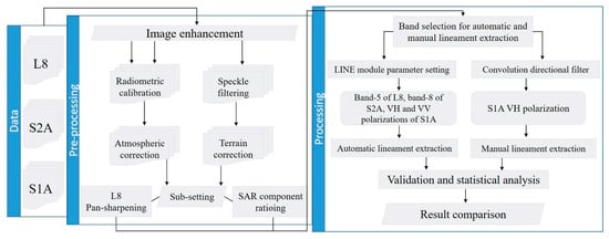
Figure 2.
The methodology flowchart of the study.
3.2.1. Landsat-8 (L8) Dataset
The geometric correction of the acquired L8 data was not necessary to be performed since it is already geometrically corrected by the United States Geological Survey (USGS) in the Universal Transfer Mercator (UTM) projection with the WGS-1984 map datum, Zone 43N. The further preprocessing of the raw L8 data, including radiometric calibration, atmospheric correction, and image normalization, was essential to performed for the dataset to be prepared for further processing. Radiometric calibration and the Fast Line-of-Sight Atmospheric Analysis of Spectral Hypercubes (FLAASH) atmospheric correction model were applied using the Environment for Visualizing Images (ENVI) software version 5.1 as it was described in the previous study [37]. Image normalization, then, was performed to this dataset in the same environment, and further sub-setting was done to extract the targeted study area. The L8 VNIR and SWIR channels with a 30 m pixel size were fused with the panchromatic channel, having a 15 m pixel size to enhance the spatial characteristics of those with lower spatial resolution. The automatic image fusion was performed using the pansharp module with no generation of a refined pansharpened image option, which is recommended for digital classification purposes [42]. The module used for image fusion is implemented in PCI Geomatica software. This image fusion technique is known as pansharpening and can be applied to the real data types (8, 16, and 32 bit). Different image fusion techniques, such as Intensity, Hue, and Saturation (IHS) are also widely used [43,44]. However, the image fusion technique used in this study tends to produce superior sharpening results, while preserving the spectral characteristics of the original images [42].
3.2.2. Sentinel-2A (S2A) Dataset
The S2A images that are used correspond to the L1C products processed by the Payload Data Ground Segment (PDGS). The provided Top-Of-Atmosphere (TOA) reflectance in cartographic geometry (UTM/WGS84) coded in JPEG2000 format data products are already processed for radiometric and geometric corrections, including orthorectification and multispectral and multi-temporal registration on a global reference system with sub-pixel accuracy [38,45]. These L1C images have usually been processed to Level-2A (L2A) data by integrating the Sen2Cor processor in the Sentinel Application Platform (SNAP) [46,47,48,49], which consists of a rich set of visualization, analysis, and processing tools for the exploitation of MSI data from the Copernicus Sentinel-2 mission. However, the L1C data was alternatively scaled to surface reflectance [50,51], using the Dark Object Subtraction (DOS) method [52,53,54,55].
In the present work, the acquired S2A L1C dataset was atmospherically corrected to the surface reflectance, using Sen2Cor atmospheric correction processor version 2.4.0 [56,57]. Sen2cor processor performs a preprocessing of the L1C TOA data product and applies a scene classification with an atmospheric, terrain, and cirrus correction and a subsequent conversion into an ortho-image L2A Bottom of Atmosphere (BOA) reflectance image data [58,59]. As it has been concluded, the higher the spatial resolution, the higher the quality of the lineament map [20]; therefore, a pixel size of 10 m for the resulting level 2A product was chosen in the correction procedure. The output BOA reflectance dataset contained bands from 2 to 7, 8, 8a, 11, and 12. The coastal aerosol-band 1 (60 m), water vapor-band 9 (60 m), and Cirrus-band 10 (60 m) were excluded by the atmospheric correction processor.
The next step was to merge the resultant corrected S2A images. The mosaicking of two or more S2A L2A multi-pixel size products with different spatial resolutions in SNAP requires the same spatial resolution for all corresponding channels. Therefore, the SWIR, Red Edge, and near-infrared (NIR) bands with a 20 m spatial resolution were first resampled using the nearest neighbor resampling method to correspond to the VNIR 10 m spatial resolution. The principle of using resampling methods is described by Tempfli, Kerle, Huurneman and Janssen [41]. Further, the datasets were mosaicked in SNAP software version 5.0.0 using Mosaic Processor. Later, the merged in a single image dataset was spatially resized in order to reduce the image size to cover only the targeted study area. Bands 5, 6, and 7 that have been utilized for the detection of vegetation red edge [49] were excluded from the dataset, leaving the VNIR and SWIR channels.
3.2.3. Sentinel 1A (S1A) Dataset
For the Interferometry Synthetic Aperture Radar (InSAR) data, the multi-looking of the S1A level-1 GRD data products was not necessary, since according to the slant ranges and azimuthal directions (5 × 1 respectively), these imageries are already multi-looked and have a homogenous number of looks which is equal to four. Moreover, these data are projected to the ground range based on the WGS84 coordinate system—the Earth ellipsoid model by the European Space Agency (ESA). The incidence angle within the provided swath ranges from 31.1° to 46.5°. The Sentinel-1 Toolbox (S1TBX) implemented in SNAP software version 5.0.0, developed by the ESA, was used to preprocess the S1A data [60].
In the preprocessing stage, firstly, speckle noise reduction filtering was applied to the S1A SAR data, allowing the preservation of the structure in the image data by filtering the homogeneous surfaces and preserving the edges, which is essential in the field of structural geology. The speckle noises in SAR images are generated by the coherent interference of waves backscattered from the rough surface of the Earth and complicate the image interpretation problem [61]. Therefore, the Refined Lee filter [62], widely used in SAR image speckle effect reduction for better backscatter analysis and visual interpretation, [49,63,64,65] was applied.
Next, for the image to geometrically represent the real Earth’s surface as close as possible and to be ready for processing and interpretation, a geocoding and orthorectification of the SAR data should be performed. To this end, terrain correction, using the Range–Doppler Terrain Correction method, was performed. To do this, the terrain correction operator of the S1TBX SAR Processing module auto-downloaded a Shuttle Radar Topography Mission (SRTM) image with a spatial resolution of 3 arc seconds (90 m), which is recommended for radar data. The resultant output from the preprocessed data contains the amplitude (A) and intensity (I) layers in both the VV and VH polarizations respectively. These two components (A and I) contain information about the amplitude and the phase of the detected signal and are stored in different layers. The (A) layer stands for the position of a point in time on a waveform cycle of a transmitted microwave signal by the sensor, while the (I) layer stands for the measured backscattered signal intensities by the sensor.
The two components derived in the previous step were combined together using the so-called ratioing technique. The ratioing is done by dividing the digital number (DN) values of each pixel in one band by the DN values of another band [66]. This technique enhances the spectral differences between the bands and reduces the shadow effects caused by topography [37,67]. Although the ratioing technique has been used mainly for optical imageries, it was suggested that the same technique can be implemented on the amplitude and intensity bands of the radar data also [41,68]. The slopes in the study area that are facing away from the sensor cannot be illuminated by the radar beam. Therefore, there is no energy that can be backscattered to the sensor, and those regions remain dark in the image [41]. Thus, the ratioing of these two components gave significant and detailed information, with a maximum contrast of lineaments over the study area. Moreover, this combination allowed us to perform the directional convolution filtering on the radar data for visual interpretation and manual lineament extraction.
3.3. Processing
3.3.1. The LINE (Lineament Extraction) Module
Automatic lineaments extraction is performed on the basis of two main processing steps. The first step is the detection of edges that give information on areas of abrupt changes in the values of neighboring pixels, while the second step is the lines detection [52,69,70]. These steps are often carried out using the LINE module of the PCI Geomatica software, which is a widely used module for automatic lineament extraction [23,71]. There are two categories of parameters applied through this module [20,69] which are listed below and govern the edge detection and curve extraction stages of the automatic lineament extraction procedure:
- (a)
- Edge detection and thresholding
- RADI (filter radius): A Gaussian filter radius used during the edge detection, measured in pixels;
- GTHR (Edge Gradient Threshold): The minimum value of gradient to be considered as an edge during the edge detection;
- (b)
- Curve extraction
- LTHR (Curve Length Threshold): The minimum length of a curve to be considered as a lineament;
- FTHR (Line Fitting Threshold): The maximum error allowed during the line segment fitting to form a lineament;
- ATHR (Angular Difference Threshold): Specifies the angle not to be exceeded between two vectors to be linked;
- DTHR (Linking Distance Threshold): The maximum distance between two vectors to be linked [69].
In the first stage mentioned above, the Canny filter is applied to produce a contour strength image. This edge detection algorithm has been proven to be a better performer than the other edge detection operators and is well-known as a good automatic edge detection technique [12,72,73]. This step is done using the radius provided by the RADI parameter. Further, the gradient is computed from the filtered image. The gradient has been thresholded with the value provided by the GTHR parameter in the second stage to obtain a binary image. In the third stage, the curves are extracted from the binary edge image. According to the value assigned in the LTHR parameter, any curve with a number of pixels smaller than the value provided in this parameter is not taken into consideration for further processing. The extracted curves are, then, converted to a vector form by fitting line segments to them. After that, polylines are generated if they respect the tolerance value defined in the FTHR parameter. Finally, two polylines are linked to form a lineament if they satisfy the criteria specified in ATHR and DTHR parameters [74].
3.3.2. Directional Filtering
Directional filtering is a spatial domain filtering technique and edge enhancement filter that selectively enhances image features having specific direction gradients [75,76,77]. Filtering consists of changing the value of a pixel based on that of its neighbors [78,79,80]. This technique is very useful in radar and optical image processing for edge enhancement, visual interpretation, and manual lineament extraction of geo-structural features using local spatial frequency. This is a widely used technique in geological applications to highlight geological structures and lineaments [8,21,70,81]. The objective aimed in the application of filters by studies was to find the best way for lineament identification and the enhancement of geo-structural information in the images corresponding to structural discontinuities [19,82,83]. Directional filtering is designed to highlight the specific characteristics of an image based on their frequency related to the texture [84]. The algorithm of directional filtering produces the first difference of the image input in the vertical, horizontal, and diagonal directions. As a result, many additional edges of diverse orientations are enhanced. Edge enhancement is performed by convolving the original data with a weighted mask or kernel [8,85,86].
3.4. Lineament Extraction
3.4.1. Automatic Lineament Extraction
The first step of automatic lineament extraction was to perform an experimental test using different value combinations for each parameter of the LINE module. The test was performed over the optical and radar datasets to select the optimal parameter settings that produced suitable output information of the lineaments extracted. The application of these parameters over the utilized data was carried out with respect to the literature and validated by visual interpretation. The default values, the proposed values, and the values defined for the LINE module parameters in this study are presented in Table 2. The second step was to select the optimal bands from the two optical datasets (L8 and S2A) that should be used for lineament extraction [20]. Each of the individual bands from these datasets was tested for automatic lineament extraction based on the ability to identify the linear segments and features over the study area using the defined optimal values of parameters. Band 5 (NIR, 1.55–1.75 μm) and band 8 (NIR, 835.1μm) from the L8 and S2A respectively were selected to be used as optimal inputs for lineament extraction. The final prepared images (L8-band 5, S2A-band 8, S1A-VH, and S1A-VV) of the study area were used as the input data for LINE module to produce the final lineament maps.
Table 2.
The values used for the parameters of the LINE module.
3.4.2. Manual Lineament Extraction
In order to evaluate the automatically extracted lineaments by the LINE module, a reference lineament map of the study area is required. The reference map for the evaluation is created based on the manual extraction of lineaments [18,87,88]. Some advantages and disadvantages of manual and automatic lineament extraction are discussed in previous studies [1,9]. However, the main advantage of manual extraction is that it is easy to distinguish the type of lineaments, whether the linear features are the tectonic origin or man-made.
Further, all seven bands of L8 and a same number of bands (VNIR and SWIR) of S2A datasets were compared in terms of the contrast and definition of geological structural features. As a result of the visual inspection, band-6 from the L8 and band-11 from the S2A datasets, which record the information at the central wavelengths of 1.6085 mm and 1.6137 mm, respectively, corresponding to the SWIR-1 channel, were selected for this stage of the study. These channels show better contrast on the geological structures compared to the other channels. The selected channels from the two used optical datasets are equivalent to band 5 of Landsat-7 which is widely used for directional filtering in numerous studies [17,81,89,90].
After that, the directional convolution filtering was applied on band 6 of L8 (Figure 3a), band 11 of S2A (Figure 3b), and VH and VV polarizations of S1A (Figure 3c,d respectively) imagery to enhance the geological structural information and to highlight the main lineament directions in the study area. The task was carried out using ENVI software version 5.1. Four principle directional filters: N–S, E–W, NE–SW, and NW–SE with a 7 × 7 kernel size were applied (Table 3). The angles of the directional filter were assigned as follows: N–S by 0°, NE–SW by 45°, E–W by 90°, and NW–SE by 135°. The kernel size selected in this study was suggested as an optimal kernel size typically used in edge enhancement [91]. The image add-back value was assigned as 60%, which specifies the percentage of the original image that is included in the output image. This part of the original image preserves the spatial context and is typically done to sharpen an image.
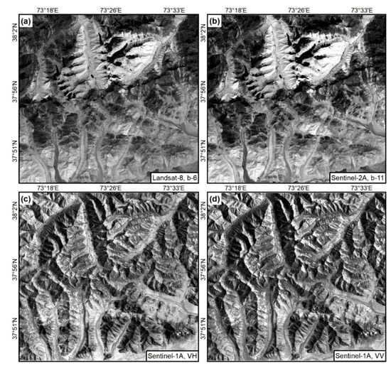
Figure 3.
The selected optical images for manual lineaments extraction for (a) L8 band-6 (SWIR) and (b) S2A band-11 (SWIR) in addition to the radar images of (c,d) S1A VH and VV polarizations respectively.
Table 3.
The four applied principle directional filters with 7 × 7 kernel matrices.
Later, the filtered images from the N–S, NE–SW, and E–W of optical and radar data were displayed in an RGB color space (Figure 4). The results show that the composed RGB image from the filtered images in the four directions of VH polarization of S1A (Figure 5) displayed a good contrast on the geological structural features such as folds and faults (Figure 4c), while the composed RGB images of optical sensors mostly highlight the lithological boundaries and with less contrast. Therefore, the RGB image composed of the filtered VH polarization (Figure 6) was selected for further manual lineament extraction. Finally, after the filtering operation and the selection of a most appropriate color composite image from the filtered images, the lineaments were defined and delineated manually with ArcMap software (version 10.3).
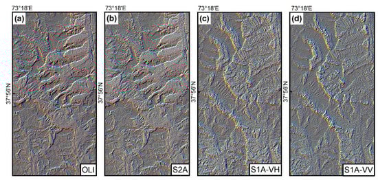
Figure 4.
The RGB composite images of three optimal filtered directions (0, 45, and 90) from (a) OLI band-6, (b) S2A band-11, and (c,d) S1A VH and VV polarizations, respectively.

Figure 5.
S1A VH polarization image filtered in the four main directions: (a) N–S direction (0), (b) NE–SW direction (45), (c) E–W direction (90), and (d) NW–SE direction (135).
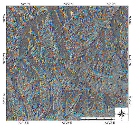
Figure 6.
The colour composite image of the three optimal filtered directions in RGB (R (0), G (45), and B (90)) of S1A VH polarization used for manual lineament extraction.
3.5. Validation
3.5.1. Shaded Relief
To verify the results, the lineaments obtained automatically using the LINE module and manually from the filtered images are spatially correlated against the shaded relief thematic map [52]. Shaded relief thematic maps are a visually pleasing representation of the terrain [92] consisting of gray values stored in raster images [92]. It assumes an illumination of the raster surface given at a defined azimuth and altitude of the sun. The boundaries between the shaded and unshaded areas may indicate the presence of lineaments [22,93]. In addition, the analysis of the shading map extracted from the Digital Elevation Model (DEM) contributes to the characterization of lineaments. Therefore, a shaded relief thematic map was derived from DEM and enhanced by applying a minimum-maximum stretch along a color ramp. After comparing the sun’s different relative position angles, the azimuth of 0° (north), which indicates the sun’s relative position along the horizon, was chosen because it can expose the shaded and unshaded areas better than other values. The altitude angle of 45°, indicating the sun’s angle of elevation above the horizon, was chosen. The task was performed using the spatial analyst hillshade tool implemented in the ArcMap software.
3.5.2. Field
A field verification survey was conducted using a Garmin® eTrex® 20 Global Positioning System (GPS) to provide accurate locations for the structural features in the study area. Several sites of geological structural features in the study area were chosen for verification that was extracted from remote sensing data through automatic and manual techniques. A field view of the geomorphology and structural elements photographed are shown in Figure 7. In addition, the extracted lineaments were compared with the faults existing in the geological map of the study area (1:200,000 scale) [94,95].
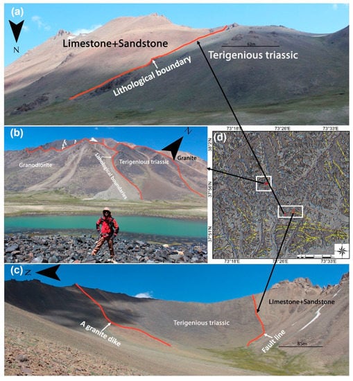
Figure 7.
Some examples of verified lineaments in the field: (a–c) Field photographs of the verified lineaments, (d) directionally filtered PGB image of S1A VH polarization with lineaments extracted (in black), verified lineaments (in red), and digitized fault lines (in yellow).
4. Results and Discussion
Image preprocessing techniques such as radiometric calibration and atmospheric correction for Landsat-8 (L8) and Sentinel-2A (S2A) satellites, pan-sharpening for L8 and mosaicing for S2A, speckle filtering and terrain correction for Sentinel-1A (S1A) satellite data as well as sub-setting applied on these images allowed us to preliminary enhance and prepare them for further analysis. For the L8 and S2A images, the comparative analysis of the used bands from these datasets in terms of the identification ability of linear features showed that the spatially enhanced band-5 (NIR) of L8 and band-8 (NIR) of S2A are the optimal bands which could be used for the auto-extraction of lineaments. This task was performed using defined optimal parameter values (Table 2). The number of automatically extracted lineaments from different bands of the L8 and S2A images is shown in Figure 8. The NIR bands of these datasets give higher lineaments number compared with visible and shortwave infrared (SWIR) bands. According to Figure 8a, the biggest number of lineaments (2338) is extracted using band-5 (NIR) of the L8 dataset. Similarly, it can be seen that the highest amount (4745) of extracted lineaments is obtained from band-8 (NIR) of S2A (Figure 8b). Therefore, these bands were considered the optimal bands for further auto-extraction of lineaments besides the two VH and VV polarization images of the radar S1A.
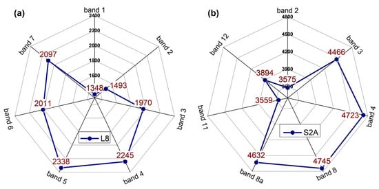
Figure 8.
Landsat-8 (a) and Sentinel-2A (b) dataset bands and the numbers of auto-extracted lineaments.
Further, the steps of automatic lineament extraction were applied over band 5, band 8, and VH and VV polarizations of the L8, S2A, and S1A images respectively, using the defined optimal parameters. The resulting extracted lineaments are then overlain to the classified geological map of the study area as shown in Figure 9a–d. The purpose of overlaying of structural information with the classified geologic map was to analyze their distribution with regards to the different existing lithological units. According to the obtained results, one can see that the lineaments extracted from the S1A VH and VV polarization images are denser and have a high concentration compared to those resulting from the L8 and S2A satellite images. For the L8 and S2A satellites, the concentration of lineaments occurs mainly in the lithological units of the study area. On the other hand, the main concentration of lineaments obtained from the VH and VV images occurs in the shadow areas, steep slopes, dikes, and structural linear features.
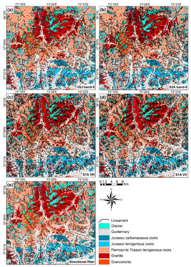
Figure 9.
The superposition of lineaments extracted automatically from (a) OLI band-5, (b) S2A band-8, and (c,d) S1A VH and VV polarizations respectively, in addition to the (e) lineaments extracted manually from the directionally filtered RGB color composite image on the Lithologic map [37].
The statistical information presented in Figure 10a–d shows that 2338 and 4745 geological lineaments were identified and extracted from the L8 and S2A images respectively, while the S1A VH and VV polarization images provide the higher number of lineaments as 5872 and 5865 respectively. According to these statistics, the values of the lineament length corresponding to the L8 range from 300 m to a maximum of 2360 m (Figure 10a). The values show a range between 200 m and around 2600 m for the S2A image (Figure 10b), while the values for the S1A VH (Figure 10c) vary between 200 m and around 2100 m and the values vary between 200 and around 2550 for the VV polarization images (Figure 10d). The maximum length for almost all four datasets is the same except the S1A VH polarization image which the maximum length is lower from those of the other images, especially the optical images having different natures. This difference shows the usefulness of the VH radar image for the automatic extraction of geological lineaments using the proposed framework.
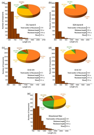
Figure 10.
The distribution histograms giving information of the number of lineaments according to the length and occupational percentage for the automatically extracted (a) OLI band-5, (b) S2A band-8, and (c,d) S1A VH and VV polarizations respectively, as well as the manually extracted (e) directionally filtered RGB color composite image.
The most abundant lineament lengths are between 300 and 400 m (1050) for the L8, 200 and 300 m (3704) for the S2A, 200 and 250 m (3131) for the S1A VH, as well as 200 and 300 m (4348) for the S1A VV that occupy 45%, 78%, 53%, and 74% of the total number of automatically extracted lineaments respectively. Comparing these numbers, it can be noted that the lineaments identified from the S1A VH polarization image are mostly characterized by smaller lengths with regards to those extracted from the other images used in this study. It, again, shows the effectiveness of the S1A VH polarization image, which is independent of the soil properties compared to the optical images [52].
For a detailed mapping of the linear structures in the study area and an evaluation of those provided through an automatic approach, directional filters were applied on the L8 band-6, S2A band-11, S1A VH, and VV polarization images. Based on the results from various color combinations, the first three principal directions (N-S, NE-SW, and E-W) were found to be more suitable for edge enhancement than the other images used in this study. Geological structures are more recognizable after a directional filtering in the VH polarization image. Therefore, the RGB color composite image was displayed to screen assigning the filtering directions derived from the VH polarization image as follows: N–S (Figure 5a) as red, NE–SW (Figure 5b) as green, and E–W (Figure 5c) as blue (Figure 6). This color composite image was used to extract the geological linear features by visual photointerpretation. [8,81]. As a result, the lineament map (Figure 9e) provided by the directional filtering technique shows a significantly lower number of lineaments compared to those obtained automatically (Figure 9 and Figure 10). However, the lineaments in this map mostly indicate the geological structural features rather than the boundaries of lithological units.
As shown in Figure 10e, in total, 1485 geological lineaments were visually identified and extracted from the filtered color composite image. The values of lineament length show a range between around 200 m and a maximum of around 3900 m. The most dominating lengths of extracted lineaments are between 300 and 500 m (476) which is 32% of the total number of extracted lineaments.
Additionally, by overlaying our automatically and manually extracted lineaments on a shaded relief thematic map, the correlation between the extracted lineaments and shading illumination was analyzed (Figure 11). The results of this analysis with a visual interpretation show that most lineaments extracted through visual interpretation from the image obtained by applying the directional filter are perfectly located between the shaded and unshaded areas (Figure 11e). It means that the obtained map can be used as a suitable reference map for the validation of those obtained by an automatic method from the radar and optical imagery. Figure 11a,b shows that the lineaments extracted from optical (L8 and S2A) data are mostly located in the boundaries between the lithological units compared to those extracted from the S1A images, which show a much less correlation with these areas (Figure 9a,b). The lineaments extracted from the S1A VH and VV polarization images (Figure 11c,d respectively) are mainly located in the slope and shading and even in the areas with no value classified as a shading area having slops and structural features, thus, indicating the high sensitivity of S1A radar data to geomorphology compared to optical L8 and S2A data.
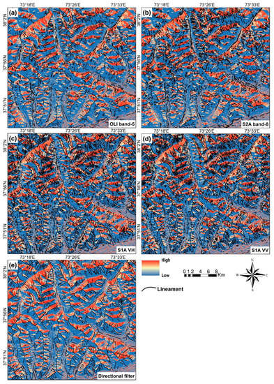
Figure 11.
The superposition of lineaments extracted automatically from (a) OLI band-5, (b) S2A band-8, and (c,d) S1A VH and VV polarizations respectively, in addition to the (e) lineaments extracted manually from the directionally filtered RGB color composite image on the Shaded relief thematic map: The colour coding denotes the shaded (high value) and unshaded (low value) areas.
4.1. Accuracy Assessment
4.1.1. Density
In lineament analysis and mapping studies, a density classification map is a parameter widely used for a correlation analysis with other geological information [4,20,73,96]. This classification map provides information about the concentration of lineaments per unit area [97]. The lineament density maps in this study are derived for each of the optical, radar, as well as manual interpretation lineament maps to analyze the dispersion pattern of the lineaments (Figure 12). The task was performed using the line density tool implemented in the ArcMap software. The higher density values in the maps are represented by a red color, while the lower values are in blue. Generally, most of the high lineament density values are located in the northern part of the images, which is mainly occupied by granites and granodiorites. These higher densities might reflect the slope angle under the lithological control. However, since granite is more compositionally and structurally homogenous than sedimentary strata that have a heterogeneous structure due to layering, one would expect smooth slopes in the areas of granite distribution and, hence, lower lineament densities. During our field campaign, this was also verified that granite slopes are smoother than the sedimentary strata. Therefore, we assume that the higher density of lineaments in the northern part of the study area could represent a higher level of deformation of rocks in this area. Moreover, the lower densities of the lineaments in the river valleys, which are the domain of quaternary deposits, suggests that deformation that is visible within the granite domain that is older than the quaternary deposits and, hence, covered by them. The analysis shows that the density maps of lineaments extracted through an automatic approach from the S1A radar images (Figure 12c,d) are highly correlated with the reference density map of lineament occurrences derived by visual interpretation (Figure 12e) rather than those from optical L8 and S2A data (Figure 12a,b respectively). The differences in lineament density patterns between optical and radar imageries is most likely related to the illumination effects, spatial resolution, and other factors that give an advantage to radar data over optical imageries.
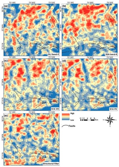
Figure 12.
The density maps of the extracted lineaments for the (a) OLI band-5, (b) S2A band-8, (c,d) S1A VH and VV polarizations respectively, and (e) the manually extracted lineaments overlain by the faults digitized from a geological map [94,95].
These density classification maps can be more useful when they are combined with other information by overlaying them on the maps. Therefore, the correlation between the density maps of the extracted lineaments and the known existing faults in the study area is also investigated through digitizing and overlaying them on the derived density maps. The density classification maps were used to find the correlation between the concentration of lineaments and the distribution of existing faults in the study area. Overlaying the existing fault map of the study area on the density maps (Figure 12a–e), it can be seen that the density maps of lineaments extracted automatically from the S1A VH and VV polarization images respectively are highly correlated with the existing faults occurrences, which is also similar with the density map provided by the manual extraction from the directional filter image (Figure 12e). An area in the northern part of the density maps, which exhibits a high lineament density but do not contain any fault, corresponds to the area of distribution of granitic bodies (Figure 9), in which the faults are hard to document due to similar lithological compositions on both sides of the fault lines. This shows that the mapping of some structural elements within the big granitic bodies using image processing techniques is even more efficient than the ground-based surveys. Amongst other obtained maps, the lineament density map of the L8 image (Figure 12a) shows the lowest correlation with the existing fault occurrences. For the optical L8 and S2A satellites, the high-density values are concentrated mainly in the northern part of the study area (Figure 12a,b), whereas the results obtained from the S1A images showed a better correlation with the distribution of the existing faults in the southern part. The directions of the faults correspond with the directions of the high-density patterns in the southern part of these maps. However, the directional correlation of faults and density patterns can also be seen in the lineament density map from the optical S2A image (Figure 12b). This analysis also proves that the results obtained from the S1A radar data are the best correlated in relation to the faults with respect to the conclusion of the shading criteria described previously.
4.1.2. Orientations
The lineament directions extracted using an automated approach can be compared with the directions relating to the manually obtained lineaments and existing faults in the study area [74,96]. Therefore, in the next accuracy assessment section, the lineament directions from the optical and radar data are compared to the directional filter image as well as the existing faults to evaluate the potential of optical L8, S2A, and S1A radar images for automatic structural lineament extraction. This allows the identification of the most frequent directions of lineaments. The lineament directions reflect the result of tectonic processes that produced them. Therefore, they also can be correlated with the geological history of the area to verify the plausibility of the obtained results.
Lineament orientation is analyzed by creating rose diagrams for each of the lineament maps including the existing faults and bedding measurements from a geological map, which present the number of lineaments dominating in a particular direction. An angular spacing of 15° without using the frequency of lineament population was set (Figure 13). As a result of the analysis, two main dominant directions are identified for each lineament set. These directions for optical data are WNW–ESE (W270–280N) and NNE–SSW (N0–10E) (Figure 13a,b). For the radar data, they are NW–SE (W310–320N) and NNE–SSW (N0–10E) (Figure 13c,d). The lineament set manually extracted from the directional filter reference image shows a trend at the WNW-ESE (W290–300N) and NNE–SSW (N0–10E) directions (Figure 13e) and for the fault set from the geological map, it is WNW-ESE (W270–280N) and NW–SE (W330–340N) (Figure 13f). Figure 13g,h demonstrates the bulk W–E direction of the strike azimuths of strata and their NNE–SSW dipping directions, respectively, which are digitized from the geological map. The rivers sometime follow the geological structural elements but mostly are the result of erosion processes, which are not necessarily related to deformation. Therefore, it is important to evaluate the contribution of drainage-controlled extracted lineaments in the rose diagram directions of the lineaments. To this end, the drainage network of the study area was extracted from an SRTM digital elevation model using the automatic watershed delineation module of the ArcSWAT model [98,99] built for the ArcMap software. The directions of the drainage network are shown in Figure 13i. As one can see on this rose diagram, the rivers are distributed in four main directions with an angle of approx. 45 degrees between each of them, which is quite natural for rivers. Comparing these directions with the lineament directions extracted from the radar data, we see that the contribution of the drainage network on the directions of the extracted lineaments is small because the lineaments’ directions have one dominant direction—NW-SE—and are not homogenously distributed in all directions.
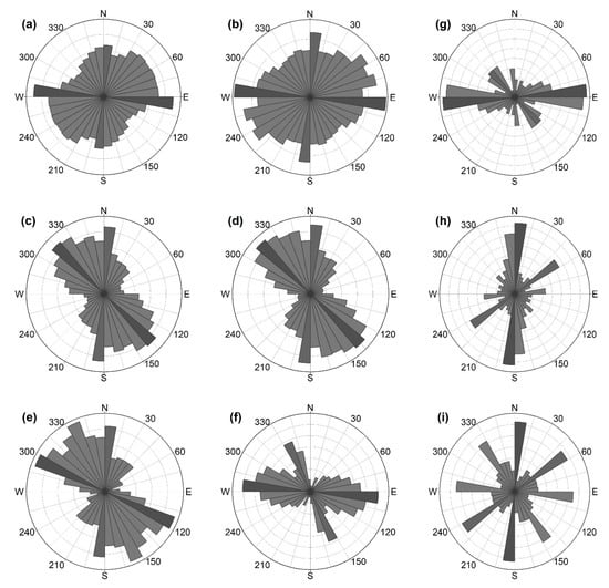
Figure 13.
Rose diagrams showing the orientations of lineaments extracted from the (a) OLI, (b) S2A, (c,d) S1A VH and VV polarizations respectively, and (e) directionally filtered images in comparison to those of (f) the faults digitized from a geologic map, (g,h) the bedding directions of strata-strike azimuths and dipping azimuths respectively, and (i) the drainage network orientations of the study area
It is interesting to note that one of the dominant directions of the faults (WNW–ESE) correlates well with one of the dominant directions of the lineaments automatically extracted from the optical imagery, while the other dominant fault direction (NW–SE) correlates with one of the lineament-dominant directions extracted from the S1A radar image. As we can see from the geological map (Figure 1b), the faults which are roughly E–W are distributed along the lithological boundaries, which are best extracted from the optical imagery because this type of imagery is more sensitive to compositional changes. This is also supported by the direction of strike azimuths, which is also roughly E–W (Figure 13g). The second dominant faults direction, which correlates with the lineaments extracted from the radar image, may indicate the main direction of the structural geological lineaments, such as faults which are not parallel to the lithological boundaries, and therefore, are not well-extracted from the optical images and best extracted from the radar image. This can also be observed on the geological map (Figure 1b), on which part of the faults striking to NW crosscut the lithological boundaries. The only dominant population of lineaments, the direction of which is the same in the optical and radar images (NNE–SSW), correlates well with the dipping direction of the geological strata and compares them with the topography and geological map; one can conclude that this direction reflects the direction of such features as watersheds and river valleys. Although, we should admit that the uneven distribution of the dipping measurements and the scarcity of the faults mapped does not allow us to excellently correlate the extracted lineaments with the geological features mapped. Therefore, a good correlation between the automatically and manually extracted lineaments is important to back up the verification of automatic lineament extraction results. The orientation analysis indicates that the major trends in the lineament maps obtained through automatic extraction from radar images have a strong correlation with the lineament map derived manually than those from optical imagery. Moreover, the lineaments extracted from the optical imagery are partly controlled by lithological units, which are not always consistent with the deformation pattern. Therefore, although the optical images generate a good number of extracted lineaments, which are parallel to the lithological boundaries, the S1A radar image is best for extracting structural lineaments.
We chose several sites of extraction from the S1A satellite image lineaments to verify during our field verification campaign, some examples of which are shown in Figure 7.
5. Conclusions
The main objective of the study was to compare the performance of optical Landsat-8 (L8) and Sentinel-2A (S2A) in addition to the Sentinel-1A (S1A) radar data in structural lineament extraction. A comparison between the different bands of optical data is also performed to select the best bands for automatic lineament extraction. The results indicate that the best bands for automatic lineament extraction are the fused band-5 (NIR) of L8 and band-8 (NIR) of the S2A. The comparison analysis of automatic lineament detection has been successful with S1A radar images performing better at identifying and extracting more lineament number with a better accuracy compared to the L8 and S2A satellite data. The S1A image resulted in 5872 and 5865 extracted lineaments from the VH and VV components respectively, whereas from the S2A and optical images, 4745 and 2338 lineaments respectively were extracted. This indicates that the optical images are 20% (S2A) and 60% (L8) less effective compared to the S1A VH component in automatic lineament extraction. This success can be attributed to S1A VH and VV polarizations and to the fact that the amplitude and intensity components of this image are combined together. Edge enhancement through directional filtering has also shown its potential to be effective in lineament visualization and their extraction using S1A VH polarization radar image compared to optical L8 and S2A imagery.
The comparison of the gained results, including the shaded relief, density maps, and rose diagrams of the extracted lineaments compared to the directional filter image and existing faults, as well as the field survey showed that the S1A data give a high number of lineaments and better results in terms of accuracy in structural lineament detection than the optical sensors. The lineaments detected from the optical L8 and S2A data follow mainly the boundaries between the lithological units, while those extracted from S1A show a strong correlation with the abrupt changes in areas of slope and shading. In addition, the lineaments extracted automatically from S1A images converge very well with the localization and the orientation of those from the directional filter image as well as existing faults in the study area. This study demonstrates that the S1A radar images not only are able to provide a high number of lineaments but also can be used for edge enhancement and visual interpretation using directional filtering techniques. These abilities demonstrate advantages of the radar S1A data over optical L8 and S2A images for structural geological studies. Consequently, the framework used in the present study has shown a great efficiency in automated lineament extraction using S1A SAR images and can be applied in surrounding areas.
Author Contributions
Conceptualization, J.A. (Javhar Aminov) and C.X.; formal analysis, J.A. (Javhar Aminov); funding acquisition, C.X.; investigation, J.A. (Javhar Aminov), J.A. (Jovid Aminov), and L.T.; methodology, J.A. (Javhar Aminov) and C.X.; supervision, C.X.; validation, J.A. (Javhar Aminov), J.A. (Jovid Aminov), and Y.M.; visualization, J.A. (Javhar Aminov) and J.A. (Jamshed Aminov); writing—original draft, J.A. (Javhar Aminov); writing—review and editing, C.X., B.A., J.A. (Jamshed Aminov), and Y.M.
Funding
This research was funded by the Strategic Priority Research Program of Chinese Academy of Sciences, Pan-Third Pole Environment Study for a Green Silk Road (Pan-TPE XDA20060303), International Cooperation Fund of Ecological Effects of Climate Change and Land Use/Cover Change in Arid and Semiarid Regions of Central Asia in the Most Recent 500 Years (Grant No. 41361140361), and Tianshan Innovation Team Project of Xinjiang Department of Science and Technology (Grant No. Y744261).
Acknowledgments
This study is the part of PhD research of Javhar Aminov and has been sponsored by the CAS-TWAS President’s Fellowship for International PhD Students awarded to him. The authors are grateful to the U.S. Geological Survey (USGS) for providing Landsat 8 and the European Space Agency (ESA) for the Sentinel 1 and 2 data.
Conflicts of Interest
The authors declare no conflict of interest.
References
- Ramli, M.F.; Yusof, N.; Yusoff, M.K.; Juahir, H.; Shafri, H.Z.M. Lineament mapping and its application in landslide hazard assessment: A review. Bull. Eng. Geol. Environ. 2010, 69, 215–233. [Google Scholar] [CrossRef]
- Negredo, A.M.; Replumaz, A.; Villaseñor, A.; Guillot, S. Modeling the evolution of continental subduction processes in the Pamir–Hindu Kush region. Earth Planet. Sci. Lett. 2007, 259, 212–225. [Google Scholar] [CrossRef]
- Mostafa, M.E.; Bishta, A.Z. Significance of lineament patterns in rock unit classification and designation: A pilot study on the Gharib-Dara area, northern Eastern Desert, Egypt. Int. J. Remote Sens. 2005, 26, 1463–1475. [Google Scholar] [CrossRef]
- Fagbohun, B.J.; Adeoti, B.; Aladejana, O.O. Litho-structural analysis of eastern part of Ilesha schist belt, Southwestern Nigeria. J. Afr. Earth Sci. 2017, 133, 123–137. [Google Scholar] [CrossRef]
- Pour, A.B.; Hashim, M. Structural geology mapping using PALSAR data in the Bau gold mining district, Sarawak, Malaysia. Adv. Space Res. 2014, 54, 644–654. [Google Scholar] [CrossRef]
- Eldosouky, A.M.; Abdelkareem, M.; Elkhateeb, S.O. Integration of remote sensing and aeromagnetic data for mapping structural features and hydrothermal alteration zones in Wadi Allaqi area, South Eastern Desert of Egypt. J. Afr. Earth Sci. 2017, 130, 28–37. [Google Scholar] [CrossRef]
- Harris, J.R. Mapping of Regional Structure of Eastern Nova Scotia Using Remotely Sensed Imagery: Implications for Regional Tectonics and Gold Exploration. Can. J. Remote Sens. 2014, 17, 122–135. [Google Scholar] [CrossRef]
- Pour, A.B.; Hashim, M. Structural mapping using PALSAR data in the Central Gold Belt, Peninsular Malaysia. Ore Geol. Rev. 2015, 64, 13–22. [Google Scholar] [CrossRef]
- Hung, L.; Batelaan, O.; Dinh, N.Q.; Lagrou, D.; de Smedt, F. Remote sensing and GIS-based analysis of cave development in the Suoimuoi catchment (Son La-NW Vietnam). J. Cave Karst Stud. 2002, 64, 23–33. [Google Scholar]
- Hung, L.; Batelaan, O. Environmental geological remote sensing and GIS analysis of tropical karst areas in Vietnam. In Proceedings of the 2003 IEEE International Geoscience and Remote Sensing Symposium (IGARSS’03), Toulouse, France, 21–25 July 2003. [Google Scholar]
- Kim, G.-B.; Lee, J.-Y.; Lee, K.-K. Construction of lineament maps related to groundwater occurrence with ArcView and Avenue™ scripts. Comput. Geosci. 2004, 30, 1117–1126. [Google Scholar] [CrossRef]
- Marghany, M.; Hashim, M. Lineament Mapping Using Multispectral Remote Sensind Data. Res. J. Appl. Sci. 2010, 5, 126–130. [Google Scholar]
- Rahnama, M.; Gloaguen, R. TecLines: A MATLAB-Based Toolbox for Tectonic Lineament Analysis from Satellite Images and DEMs, Part 1: Line Segment Detection and Extraction. Remote Sens. 2014, 6, 5938–5958. [Google Scholar] [CrossRef]
- Geological Applications of LANDSAT Thematic Mapper Imagery: Mapping and Analysis of Lineaments in NW Penisula Malaysia. Available online: https://www.geospatialworld.net/article/geological-applications-of-landsat-thematic-mapper-imagery-mapping-and-analysis-of-lineaments-in-nw-penisula-malaysia/ (accessed on 26 March 2019).
- Abdullah, A.; Nassr, S.; Ghaleeb, A. Remote Sensing and Geographic Information System for Fault Segments Mapping a Study from Taiz Area, Yemen. J. Geol. Res. 2013, 2013, 1–16. [Google Scholar] [CrossRef]
- Argialas, D.; Ourania, M.; Stefouli, M. Automatic mapping of tectonic lineaments (faults) using methods and techniques of Photointerpretation/Digital Remote Sensing and Expert Systems. THALES Project 2000, 4. [Google Scholar]
- Kavak, K.S. Determination of palaeotectonic and neotectonic features around the Menderes Massif and the Gediz Graben (western Turkey) using Landsat TM image. Int. J. Remote Sens. 2005, 26, 59–78. [Google Scholar] [CrossRef]
- Suzen, M.L.; Toprak, V. Filtering of satellite images in geological lineament analyses: An application to a fault zone in Central Turkey. Int. J. Remote Sens. 1998, 19, 1101–1114. [Google Scholar] [CrossRef]
- Ali, S.A.; Pirasteh, S. Geological applications of Landsat Enhanced Thematic Mapper (ETM) data and Geographic Information System (GIS): Mapping and structural interpretation in south-west Iran, Zagros Structural Belt. Int. J. Remote Sens. 2004, 25, 4715–4727. [Google Scholar] [CrossRef]
- Hung, L.Q.; Batelaan, O.; de Smedt, F. Lineament extraction and analysis, comparison of LANDSAT ETM and ASTER imagery. Case study: Suoimuoi tropical karst catchment. Vietnam 2005, 5983, 59830T. [Google Scholar]
- Kocal, A.; Duzgun, H.; Karpuz, C. Discontinuity Mapping with Automatic Lineament Extraction from High Resolution Satellite Imagery. In Proceedings of the XXth ISPRS Congress, Istanbul, Turkey, 12–23 July 2004. [Google Scholar]
- Masoud, A.; Koike, K. Tectonic architecture through Landsat-7 ETM+/SRTM DEM-derived lineaments and relationship to the hydrogeologic setting in Siwa region, NW Egypt. J. Afr. Earth Sci. 2006, 45, 467–477. [Google Scholar] [CrossRef]
- Qari, M.H. Lineament extraction from multi-resolution satellite imagery: A pilot study on Wadi Bani Malik, Jeddah, Kingdom of Saudi Arabia. Arabian J. Geosci. 2010, 4, 1363–1371. [Google Scholar] [CrossRef]
- Grebby, S.; Cunningham, D.; Naden, J.; Tansey, K. Application of airborne LiDAR data and airborne multispectral imagery to structural mapping of the upper section of the Troodos ophiolite, Cyprus. Int. J. Earth Sci. 2011, 101, 1645–1660. [Google Scholar] [CrossRef]
- Jordan, G.; Schott, B. Application of wavelet analysis to the study of spatial pattern of morphotectonic lineaments in digital terrain models. A case study. Remote Sens. Environ. 2005, 94, 31–38. [Google Scholar] [CrossRef]
- Irons, J.R.; Loveland, T.R. Eighth Landsat satellite becomes operational. Photogramm. Eng. Remote Sens. 2013, 79, 398–401. [Google Scholar]
- Berger, M.; Moreno, J.; Johannessen, J.A.; Levelt, P.F.; Hanssen, R.F. ESA’s sentinel missions in support of Earth system science. Remote Sens. Environ. 2012, 120, 84–90. [Google Scholar] [CrossRef]
- Burtman, V.S.; Molnar, P.H. Geological and Geophysical Evidence for Deep Subduction of Continental Crust Beneath the Pamir; Geological Society of America: Boulder, CO, USA, 1993; Volume 281. [Google Scholar]
- Angiolini, L.; Zanchi, A.; Zanchetta, S.; Nicora, A.; Vezzoli, G. The Cimmerian geopuzzle: New data from South Pamir. Terra Nova 2013, 25, 352–360. [Google Scholar] [CrossRef]
- Burtman, V. Tien Shan, Pamir, and Tibet: History and geodynamics of Phanerozoic oceanic basins. Geotectonics 2010, 44, 388–404. [Google Scholar] [CrossRef]
- Robinson, A.C. Mesozoic tectonics of the Gondwanan terranes of the Pamir plateau. J. Asian Earth Sci. 2015, 102, 170–179. [Google Scholar] [CrossRef]
- Aminov, J.; Ding, L.; Mamadjonov, Y.; Dupont-Nivet, G.; Aminov, J.; Zhang, L.; Yoqubov, S.; Aminov, J.; Abdulov, S. Pamir Plateau formation and crustal thickening before the India-Asia collision inferred from dating and petrology of the 110–92 Ma Southern Pamir volcanic sequence. Gondwana Res. 2017, 51, 310–326. [Google Scholar] [CrossRef]
- Hu, X.; Garzanti, E.; Wang, J.; Huang, W.; An, W.; Webb, A. The timing of India-Asia collision onset–Facts, theories, controversies. Earth-Sci. Rev. 2016, 160, 264–299. [Google Scholar] [CrossRef]
- Sippl, C.; Schurr, B.; Yuan, X.; Mechie, J.; Schneider, F.M.; Gadoev, M.; Orunbaev, S.; Oimahmadov, I.; Haberland, C.; Abdybachaev, U.; et al. Geometry of the Pamir-Hindu Kush intermediate-depth earthquake zone from local seismic data. J. Geophys. Res. Solid Earth 2013, 118, 1438–1457. [Google Scholar] [CrossRef]
- Schurr, B.; Ratschbacher, L.; Sippl, C.; Gloaguen, R.; Yuan, X.; Mechie, J. Seismotectonics of the Pamir. Tectonics 2014, 33, 1501–1518. [Google Scholar] [CrossRef]
- Stübner, K.; Ratschbacher, L.; Rutte, D.; Stanek, K.; Minaev, V.; Wiesinger, M.; Gloaguen, R. Project TIPAGE Members. The giant Shakhdara migmatitic gneiss dome, Pamir, India-Asia collision zone: 1. Geometry and kinematics. Tectonics 2013, 32, 948–979. [Google Scholar] [CrossRef]
- Aminov, J.; Chen, X.; Aminov, J.; Mamadjanov, Y.; Aminov, J.; Duulatov, E.; Bakhtiyorov, Z. Evaluation of Remote Sensing Techniques for Lithological Mapping in the Southeastern Pamir using Landsat 8 OLI Data. Int. J. Geoinform. 2018, 14, 1–10. [Google Scholar]
- Gascona, F.; Cadau, E.; Colin, O.; Hoersch, B.; Isola, C.; Fernández, B.L.; Martimort, P. Copernicus Sentinel-2 mission: Products, algorithms and cal/val. In Proceedings of the SPIE, San Diego, CA, USA, 26 September 2014. [Google Scholar]
- Geudtner, D.; Torres, R.; Snoeij, P.; Davidson, M.; Rommen, B. Sentinel-1 system capabilities and applications. In Proceedings of the 2014 IEEE International Conference on Geoscience and Remote Sensing Symposium (IGARSS), Quebec City, QC, Canada, 13–18 July 2014. [Google Scholar]
- The Copernicus Open Access Hub Website. Available online: https://scihub.copernicus.eu/ (accessed on 19 October 2017).
- Tempfli, K.; Kerle, N.; Huurneman, G.C.; Janssen, L.L. Principles of Remote Sensing, 4th ed.; The International Institute for Geo-Information Science and Earth Observation, (ITC): Enschede, The Netherlands, 2009. [Google Scholar]
- Zhang, Y. A new automatic approach for effectively fusing Landsat 7 as well as IKONOS images. In Proceedings of the 2002 IEEE International Conference on Geoscience and Remote Sensing Symposium (IGARSS’02), Toronto, ON, Canada, 24–28 June 2002. [Google Scholar]
- Mwaniki, M.W.; Moeller, M.S.; Schellmann, G. A comparison of Landsat 8 (OLI) and Landsat 7 (ETM+) in mapping geology and visualising lineaments: A case study of central region Kenya. ISPRS—International Archives of the Photogrammetry. Remote Sens. Spat. Inf. Sci. 2015, XL-7/W3, 897–903. [Google Scholar]
- Mwaniki, M.W.; Matthias, M.S.; Schellmann, G. Application of remote sensing technologies to map the structural geology of central Region of Kenya. IEEE J. Sel. Top. Appl. Earth Obs. Remote Sens. 2015, 8, 1855–1867. [Google Scholar] [CrossRef]
- Dechoz, C.; Poulain, V.; Massera, S.; Languille, F.; Greslou, D.; de Lussy, F.; Gaudel, A.; L’Helguen, C.; Picard, C.; Trémas, T. Sentinel 2 global reference image. In Image and Signal Processing for Remote Sensing XXI; SPIE: Bellingham, WA, USA, 2015. [Google Scholar]
- van der Werff, H.; van der Meer, F. Sentinel-2A MSI and Landsat 8 OLI Provide Data Continuity for Geological Remote Sensing. Remote Sens. 2016, 8, 883. [Google Scholar] [CrossRef]
- Roy, D.P.; Li, J.; Zhang, H.K.; Yan, L.; Huang, H.; Li, Z. Examination of Sentinel-2A multi-spectral instrument (MSI) reflectance anisotropy and the suitability of a general method to normalize MSI reflectance to nadir BRDF adjusted reflectance. Remote Sens. Environ. 2017, 199, 25–38. [Google Scholar] [CrossRef]
- Navarro, G.; Caballero, I.; Silva, G.; Parra, P.; Vázquez, Á.; Caldeira, R. Evaluation of forest fire on Madeira Island using Sentinel-2A MSI imagery. Int. J. Appl. Earth Obs. Geoinf. 2017, 58, 97–106. [Google Scholar] [CrossRef]
- Castillo, J.A.A.; Apan, A.A.; Maraseni, T.N.; Salmo, S.G., III. Estimation and mapping of above-ground biomass of mangrove forests and their replacement land uses in the Philippines using Sentinel imagery. ISPRS J. Photogramm. Remote Sens. 2017, 134, 70–85. [Google Scholar] [CrossRef]
- Fernández-Manso, A.; Fernández-Manso, O.; Quintano, C. SENTINEL-2A red-edge spectral indices suitability for discriminating burn severity. Int. J. Appl. Earth Obs. Geoinf. 2016, 50, 170–175. [Google Scholar] [CrossRef]
- Chrysafis, I.; Mallinis, G.; Siachalou, S.; Patias, P. Assessing the relationships between growing stock volume and Sentinel-2 imagery in a Mediterranean forest ecosystem. Remote Sens. Lett. 2017, 8, 508–517. [Google Scholar] [CrossRef]
- Adiri, Z.; el Harti, A.; Jellouli, A.; Lhissou, R.; Maacha, L.; Azmi, M.; Zouhair, M.; Bachaoui, M.E. Comparison of Landsat-8, ASTER and Sentinel 1 satellite remote sensing data in automatic lineaments extraction: A case study of Sidi Flah-Bouskour inlier, Moroccan Anti Atlas. Adv. Space Res. 2017, 60, 2355–2367. [Google Scholar] [CrossRef]
- Chavez, P.S. An improved dark-object subtraction technique for atmospheric scattering correction of multispectral data. Remote Sens. Environ. 1988, 24, 459–479. [Google Scholar] [CrossRef]
- Zhang, Z.; He, G.; Wang, X. A practical DOS model-based atmospheric correction algorithm. Int. J. Remote Sens. 2010, 31, 2837–2852. [Google Scholar] [CrossRef]
- Chrysoulakis, N.; Abrams, M.; Feidas, H.; Arai, K. Comparison of atmospheric correction methods using ASTER data for the area of Crete, Greece. Int. J. Remote Sens. 2010, 31, 6347–6385. [Google Scholar] [CrossRef]
- European Space Agency, Level-2A Prototype Processor for Atmosphericterrain and Cirrus Correction of Top-of-Atmosphere Level 1C Input Data. Available online: http://step.esa.int/main/third-party-plugins-2/sen2cor/ (accessed on 22 October 2017).
- Main-Knorn, M.; Pflug, B.; Debaecker, V.; Louis, J. CALIBRATION AND VALIDATION PLAN FOR THE L2A PROCESSOR AND PRODUCTS OF THE SENTINEL-2 MISSION. Int. Arch. Photogramm. Remote Sens. Spatial Inf. Sci. 2015, 7, 1249–1255. [Google Scholar] [CrossRef]
- Muller-Wilm, U.; Louis, J.; Richter, R.; Gascon, F. Sentinel-2 level 2A prototype processor: Architecture, algorithms and first results. In Proceedings of the 2013 ESA Living Planet Symposium, Edinburgh, UK, 2013. [Google Scholar]
- Müller-Wilm, U. Sentinel-2 MSI—Level-2A Prototype Processor Installation and User Manual; Telespazio VEGA Deutschland GmbH: Darmstadt, Germany, 2016. [Google Scholar]
- Sentinel-1 Toolbox, S.T. Available online: https://sentinels.copernicus.eu/web/sentinel/toolboxes/sentinel-1 (accessed on 22 October 2017).
- Lee, J.S.; Mitchell, G.R.; Gianfranco, D.G. Polarimetric SAR Speckle Filtering and Its Implication for Classificatio. IEEE Trans. Geosci. Remote Sens. 1999, 37, 2363–2373. [Google Scholar]
- Lee, J.S. Refined Filtering of Image Noise Using Local Statistics. Comput. Graph. Image Process. 1981, 15, 380–389. [Google Scholar] [CrossRef]
- Attarzadeh, R.; Amini, J.; Notarnicola, C.; Greifeneder, F. Synergetic Use of Sentinel-1 and Sentinel-2 Data for Soil Moisture Mapping at Plot Scale. Remote Sens. 2018, 10, 1285. [Google Scholar] [CrossRef]
- Tsyganskaya, V.; Martinis, S.; Marzahn, P.; Ludwig, R. Detection of Temporary Flooded Vegetation Using Sentinel-1 Time Series Data. Remote Sens. 2018, 10, 1286. [Google Scholar] [CrossRef]
- Chatziantoniou, A.; Psomiadis, E.; Petropoulos, G. Co-Orbital Sentinel 1 and 2 for LULC Mapping with Emphasis on Wetlands in a Mediterranean Setting Based on Machine Learning. Remote Sen. 2017, 9, 1259. [Google Scholar] [CrossRef]
- Madani, A.A.; Emam, A.A. SWIR ASTER band ratios for lithological mapping and mineral exploration: A case study from El Hudi area, southeastern desert, Egypt. Arabian J. Geosci. 2009, 4, 45–52. [Google Scholar] [CrossRef]
- Nalbant, S.S.; AlpteklN, Ö. The use of Landsat Thematic Mapper imagery for analysing lithology and structure of Korucu-Du[ggrave] la area in western Turkey. Int. J. Remote Sens. 1995, 16, 2357–2374. [Google Scholar] [CrossRef]
- Heine, I.; Jagdhuber, T.; Itzerott, S. Classification and monitoring of reed belts using dual-polarimetric TerraSAR-X time series. Remote Sens. 2016, 8, 552. [Google Scholar] [CrossRef]
- Abdullah, A.; Nassr, S.; Ghaleeb, A. Landsat ETM-7 for lineament mapping using automatic extraction technique in the SW part of Taiz Area, Yemen. Glob. J. Hum.-Soc. Sci. Res. 2013, 13, 35–38. [Google Scholar]
- Thannoun, R.G. Automatic extraction and geospatial analysis of lineaments and their tectonic significance in some areas of Northern Iraq using remote sensing techniques and GIS. Int. J. Enhanc. Res. Sci. Technol. Eng. Bull. 2013, 2. [Google Scholar] [CrossRef]
- Abdullah, A.; Akhir, J.M.; Abdullah, I. Automatic mapping of lineaments using shaded relief images derived from digital elevation model (DEMs) in the Maran–Sungi Lembing area, Malaysia. Electron. J. Geotech. Eng. 2010, 15, 1–9. [Google Scholar]
- Maini, R.; Aggarwal, H. Study and comparison of various image edge detection techniques. Int. J. Image Process. (IJIP) 2009, 3, 1–11. [Google Scholar]
- Corgne, S.; Magagi, R.; Yergeau, M.; Sylla, D. An integrated approach to hydro-geological lineament mapping of a semi-arid region of West Africa using Radarsat-1 and GIS. Remote Sens. Environ. 2010, 114, 1863–1875. [Google Scholar] [CrossRef]
- Hashim, M.; Ahmad, S.; MdJohari, M.A.; Pour, A.B. Automatic lineament extraction in a heavily vegetated region using Landsat Enhanced Thematic Mapper (ETM+) imagery. Adv. Space Res. 2013, 51, 874–890. [Google Scholar] [CrossRef]
- Carr, J.R. Numerical analysis for the geological sciences. Estud. Geográficos 1996, 57, 166. [Google Scholar]
- Haralick, R.M.; Sternberg, S.R.; Zhuang, X. Image analysis using mathematical morphology. IEEE Trans. Pattern Anal. Mach. Intell. 1987, PAMI-9, 532–550. [Google Scholar] [CrossRef]
- Vincent, R.K. Fundamentals of Geological and Environmental Remote Sensing; Prentice Hall: Upper Saddle River, NJ, USA, 1997; Volume 366. [Google Scholar]
- Touzi, R.; Lopes, A.; Bousquet, P. A statistical and geometrical edge detector for SAR images. IEEE Trans. Geosci. Remote Sens. 1988, 26, 764–773. [Google Scholar] [CrossRef]
- Nezry, E.; Lopes, A.; Touzi, R. Detection of structural and textural features for SAR images filtering. In Proceedings of the 11th Annual International Geoscience and Remote Sensing Symposium (IGARSS’91), Valencia, Spain, 23–27 July 2018. [Google Scholar]
- Lopes, A.; Nezry, E.; Touzi, R.; Laur, H. Structure detection and statistical adaptive speckle filtering in SAR images. Int. J. Remote Sens. 1993, 14, 1735–1758. [Google Scholar] [CrossRef]
- Amri, K.; Mahdjoub, Y.; Guergour, L. Use of Landsat 7 ETM+ for lithological and structural mapping of Wadi Afara Heouine area (Tahifet–Central Hoggar, Algeria). Arabian J. Geosci. 2010, 4, 1273–1287. [Google Scholar] [CrossRef]
- Ali, E.A. Landsat ETM+7 Digital Image Processing Techniques for Lithological and Structural Lineament Enhancement: Case Study Around Abidiya Area, Sudan. Open Remote Sens. J. 2012, 5, 83–89. [Google Scholar] [CrossRef]
- Krishnamurthy, J. The evaluation of digitally enhanced Indian Remote Sensing Satellite (IRS) data for lithological and structural mapping. Int. J. Remote Sens. 1997, 18, 3409–3437. [Google Scholar] [CrossRef]
- Himyari, M.; Hoepffner, C.; Benzakour, M.; Hadani, E.D.E.L. Etude structurale du haut atlas oriental Maroc) à l’aide de l’analyse linéamentaire des images HRV XS) de Spot. Télédétection 2002, 2, 243–253. [Google Scholar]
- Safari, H.O.; Pirasteh, S.; Mansor, S.B. Role of the Kazerun fault for localizing oil seepage in the Zagros Mountain, Iran: An application of GiT. Int. J. Remote Sens. 2011, 32, 1–16. [Google Scholar] [CrossRef]
- Pirasteh, S.; Pradhan, B.; Safari, H.O.; Ramli, M.F. Coupling of DEM and remote-sensing-based approaches for semi-automated detection of regional geostructural features in Zagros mountain, Iran. Arabian J. Geosci. 2013, 6, 91–99. [Google Scholar] [CrossRef]
- Koike, K.; Nagano, S.; Ohmi, M. Lineament analysis of satellite images using a segment tracing algorithm (STA). Comput. Geosci. 1995, 21, 1091–1104. [Google Scholar] [CrossRef]
- Novak, I.; Soulakellis, N. Identifying geomorphic features using LANDSAT-5/TM data processing techniques on Lesvos, Greece. Geomorphology 2000, 34, 101–109. [Google Scholar] [CrossRef]
- Allou, G.; Ouattara, G.; Coulibaly, Y.; Bonin, B. The landsat 7 etm+ remote sensing imagery for lithological and structural mapping in the central côte d’ivoire (west africa): Case of dabakala. AREA Eur. Sci. J. 2015, 11. [Google Scholar] [CrossRef]
- Rawashdeh, S.A.; Saleh, B.; Hamzah, M. The use of remote sensing technology in geological investigation and mineral detection in El Azraq-Jordan. Cybergeo: Eur. J. Geogr. 2006. [Google Scholar] [CrossRef]
- Chavez, P., Jr.; Bauer, B. An automatic pptimum kernel-size selection technique for edge enhancement. Remote Sens. Environ. 1982, 12, 23–38. [Google Scholar] [CrossRef]
- Marston, B.E.; Jenny, B. Improving the representation of major landforms in analytical relief shading. Int. J. Geogr. Inf. Sci. 2015, 29, 1144–1165. [Google Scholar] [CrossRef]
- Saadi, N.M.; AbdelZaher, M.; El-Baz, F.; Watanabe, K. Integrated remote sensing data utilization for investigating structural and tectonic history of the Ghadames Basin, Libya. Int. J. Appl. Earth Obs. Geoinf. 2011, 13, 778–791. [Google Scholar] [CrossRef]
- Denykaev, S.S. Geological map of the SSR (200k scale; sheet # J-43-XX, XXVI). 1966. [Google Scholar]
- Voskonyanc, G.S. Geological map of the SSR (200k scale; sheet # J-43-XIV). 1966. [Google Scholar]
- Farahbakhsh, E.; Chandra, R.; Olierook, H.K.; Scalzo, R.; Clark, C.; Reddy, S.M.; Muller, R.D. Computer vision-based framework for extracting geological lineaments from optical remote sensing data. arXiv, 2018; arXiv:1810.02320. [Google Scholar]
- Mostafa, M.E.; Qari, M.Y.H. An exact technique of counting lineaments. Eng. Geol. 1995, 39, 5–15. [Google Scholar] [CrossRef]
- Khalid, C. Hydrological modeling of the Mikkés watershed (Morocco) using ARCSWAT model. Sustain. Water Resour. Manag. 2018, 4, 105–115. [Google Scholar] [CrossRef]
- Molina-Navarro, E.; Nielsen, A.; Trolle, D. A QGIS plugin to tailor SWAT watershed delineations to lake and reservoir waterbodies. Environ. Model. Softw. 2018, 108, 67–71. [Google Scholar] [CrossRef]


© 2019 by the authors. Licensee MDPI, Basel, Switzerland. This article is an open access article distributed under the terms and conditions of the Creative Commons Attribution (CC BY) license (http://creativecommons.org/licenses/by/4.0/).