Monitoring 3D Building Change and Urban Redevelopment Patterns in Inner City Areas of Chinese Megacities Using Multi-View Satellite Imagery

Abstract

Inner-city redevelopment is regarded as an effective way to promote land-use efficiency and optimize land-use structure, especially with the establishment of urban growth boundaries in Chinese cities. However, inner-city redevelopment as compared to urban sprawl has been rarely monitored in 2D space, let alone in 3D space. Therefore, in this paper, a novel approach to generate time-series 3D building maps (i.e., building footprint and height) based on high-resolution (2 m) multi-view ZY-3 satellite imagery was proposed. In the proposed method, the building footprint was updated by an object-based image-to-map change detection method, which employed spectral (i.e., HSV and NDVI) and structural features (i.e., morphological building index) to extract non-building and building objects, respectively; building height was estimated automatically through semi-global matching of multi-view images. We applied the proposed method to four representative Chinese megacities, i.e., Beijing, Xi’an, Shanghai, and Wuhan, for the period 2012–2017, and detected building footprints with overall accuracies ranging from 84.84% to 97.60%. The building height estimation was also relatively accurate, with the bias, slope, and root-mean-square error being −0.49–2.30 m, 0.93–1.10 m, and 4.94–7.31 m, respectively. Our results show that the total building coverage decreased over the study period, accompanied by an increase in both area-weighted building height and floor area ratio. In addition, compact low-rise buildings have been replaced by open high-rise buildings in the urban redevelopment process. Moreover, due to the scattered spatial distribution of the redevelopment sites, the local spatial aggregation patterns of building density are unlikely to shift between hotspots (i.e., spatial aggregation of high values) and coldspots (i.e., spatial aggregation of low values).

1. Introduction

The developing world has experienced unprecedentedly rapid urbanization in recent decades. In the recently released National New-Type Urbanization Plan (2014–2020), the urbanization rate of the residential population in China was 53.7% in 2013 [1]. The urbanization rate was projected to grow to about 60.0% in 2020 [1]. The demand for urban space to host the increased population has surged in China, leading to a development pattern with a mixture of urban fringe expansion and inner-city redevelopment. The urban expansion elasticity coefficient, which is defined as the ratio of growth rate of urban land to that of urban population, was 1.85 for China during 2000–2010, which was almost double the “reasonable value” (1.12) suggested by the China Academy of Urban Planning and Design [2]. This indicates extensive and low-efficiency urban sprawl. In addition, urban expansion can lead to widespread ecological and land degradation, and issues such as farmland occupation [3], lake shrinkage [4], vegetation loss [5,6], food security [7,8], air pollution [9], and the urban heat island effect [10], which have raised serious concerns for both government and the general public. Under this background, the government of China is starting to delimit “ecological control lines” [11], “red lines” for arable land [12], and “urban growth boundaries” [13] to protect China’s limited ecological land and arable land and avoid blind expansion (i.e., blind pursuit of large-scale city construction without considering practical conditions). Under the restriction of urban expansion, redevelopment of existing urban land becomes a good alternative to create more urban space.

Recently, many Chinese cities such as Beijing and Shanghai have been entering the era of urban redevelopment. As suggested by the Beijing-Tianjin-Hebei Coordinated Development Plan [14], in order to free up more space for capital functions in Beijing, non-capital functions, such as general manufacturing, business, educational and medical services, should be relocated away from the city center [15]. According to the newly released Shanghai Master Plan (2017–2035), which has been approved by China’s State Council, the overall area of construction land should realize negative growth, and the population size should be strictly controlled [16]. For these cities, urban redevelopment has been encouraged in the existing built-up areas, especially in the inner city, and urban expansion has been strictly controlled. In addition, the “stock priority” (i.e., priority to revitalize the stock land) highlighted by the National New-type Urbanization Plan (2014–2020) suggests that land supply in China will change from incremental expansion into stock land redevelopment [17].

A large number of remote sensing studies have focused on urban expansion at regional [18,19,20], national [21,22,23], continental [24,25,26], and global scales [27,28,29]. However, the analysis of inner-city redevelopment has rarely been addressed. Three typical redevelopment projects in Hong Kong were investigated by Wang et al. (2014) [30] to reveal the practical operations and key factors involved in the redevelopment plans, in an empirical study based on data acquired from the Urban Renewal Authority. Based on Landsat data, the change caused by urban expansion and renewal was detected and analyzed by Shahtahmassebi et al. (2016) [31]. Using time-series high-resolution remote sensing satellite data, Zhang and Huang (2018) [32] investigated impervious surface change in Shenzhen’s inner city during 2003–2017, and Lefebvre and Corpetti (2017) [33] monitored the urban pattern transformation of Beijing Old City from 1969 to 2015. Nevertheless, the above-mentioned studies focused on 2D urban change analysis, and they did not describe the micro-scale inner-city redevelopment process in 3D space.

Due to the difficulty of 3D urban data acquisition, little progress has been made in addressing 3D urban change, not to mention 3D urban redevelopment. Zambon et al. (2019) [34] investigated urban horizontal and vertical growth based on the official statistics of building activity (number of floors and construction age). Frolking et al. (2013) [29] used urban backscatter and nighttime lights data to indicate the macro-scale 3D urban trajectory at a very coarse resolution (i.e., 5 km). Zhang et al. (2017) [35] detected horizontal and vertical urban growth using Landsat imagery (30 m). However, the relatively low spatial resolution of these studies has limited their ability to quantify micro-scale 3D change and redevelopment patterns. In the current literature, a considerable amount of research has already addressed high-resolution 3D data generation, e.g., using synthetic aperture radar (SAR) [36], light detection and ranging (LiDAR) [37], and stereo optical imagery [38]. However, SAR data suffer from speckle noise due to the mutual interference of the surrounding structures, which makes it difficult to estimate building height in complex urban scenes [39]. In contrast, LiDAR provides highly accurate ranging measurements, but is significantly more expensive, especially for frequent monitoring of a large geographic area. In this context, the photogrammetric measurement of stereo optical imagery provides a feasible and promising approach for height estimation [38].

Although remote sensing imagery has been widely used in change detection and analysis, most of the studies have only been concerned with change at the frequency of several years or decades [40,41,42]. Change detection at a very coarse temporal interval may not accurately describe the change process, especially for high temporal dynamics, such as urban expansion and urban redevelopment.

To sum up, time-series 3D urban redevelopment is urgently required. The high-resolution multi-view (forward, nadir, and backward view) ZY-3 01 and 02 satellites provide a 3-day revisit cycle for frequent image coverage. The easily available time-series high-resolution multi-view imagery provided by the ZY-3 satellites has made it possible to conduct analysis of 3D inner-city redevelopment [38,43,44]. In this context, a framework to generate time-series 3D building maps was proposed and 3D inner-city redevelopment patterns were quantitatively analyzed. The time-series 3D building maps are updated from pre-existing 3D building maps in 2012. Please note that the pre-existing 3D maps lack time-series information to track the annual dynamics, making it impossible to monitor the rapid urban change. Therefore, using time-series multi-view ZY-3 imagery, image-to-map change detection was performed to update the temporally inconsistent information by automatically detecting building/non-building objects in the satellite image regions labeled as non-building/building in the pre-existing maps, which avoids the need for classification of all the objects over the whole image. The proposed method was carried out in the four Chinese megacities of Beijing, Xi’an, Shanghai, and Wuhan, for 2012–2017. Based on the generated time-series 3D building data, we attempted to:

(i)

explore the 3D change over the study areas;

(ii)

quantify the annual change rate of building size, height, volume, and span;

(iii)

analyze the change characteristics in different urban functional zones; and

(iv)

assess the impact of urban redevelopment on the spatial autocorrelation of 2D and 3D building density.

The outcome of this research will support automatic time-series 3D data generation and help us to understand how inner-city areas have changed under urban redevelopment.

2. Methodology

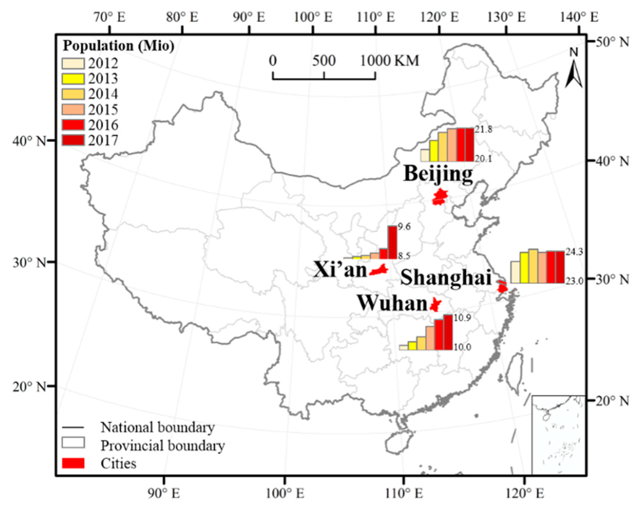
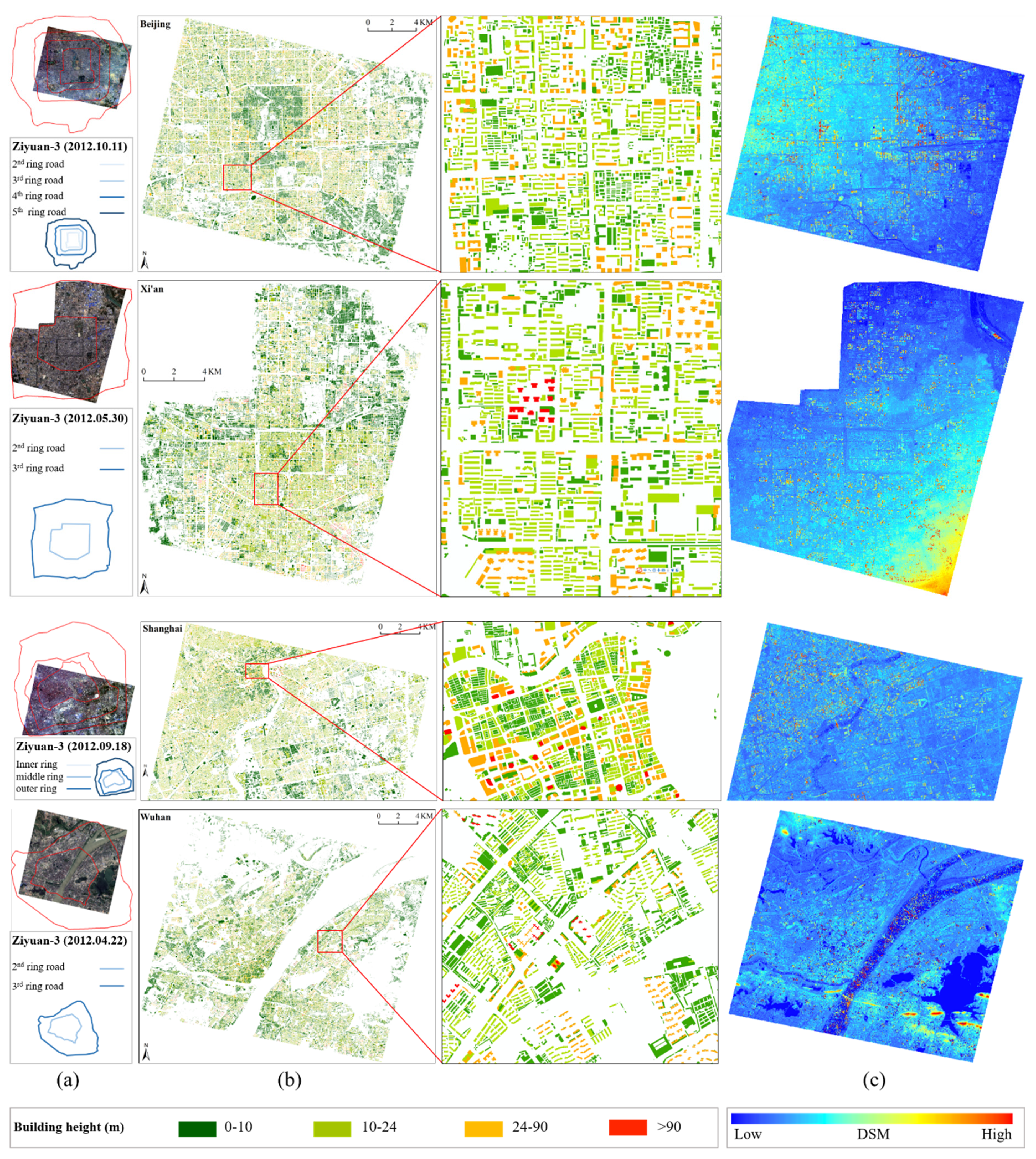
2.1. Study Areas and Data Sets

2.1.1. Study Areas

The inner-city areas of the four Chinese megacities, i.e., Beijing, Shanghai, Wuhan, and Xi’an, located in the north, east, center, and west of China, respectively, were selected as our study areas (Figure 1). Beijing in the Bohai Economic Rim, Shanghai in the Yangtze River Delta Economic Zone, Xi’an in the West Triangle Economic Zone, and Wuhan in the Yangtze River Mid-Reaches Metropolitan Region represent four of the nine National Central Cities of China. The National Central Cities, as designated by the Ministry of Housing and Urban-Rural Development of China, are the regional centers of finance, trade, culture, and management. The National Central Cities not only bear the responsibility of promoting the development of the surrounding cities, but also improving their own urbanization quality. Beijing and Shanghai have already become international cities, and they will serve as the centers for global innovation and core cities of world-class urban agglomerations [45]. Xi’an and Wuhan have become national innovation-oriented centers [45]. The GDP of Beijing, Shanghai, Xi’an, and Wuhan accounted for 3.41%, 3.73%, 0.91%, and 1.63% of China, respectively [46]. By investigating the general characteristics of 3D inner-city redevelopment in these study areas, effective guidance can be provided for other cities.

Beijing, as the capital of China, has experienced rapid growth in both built-up area and urban population since the 1980s, although the rate of population increase has slowed down since 2015 [46]. In addition, due to the excessive concentration of urban functions in Beijing’s inner city, 60% of the permanent population reside in this area, resulting in the “big city diseases” of traffic congestion, resource shortages, housing problems, etc. [47]. The adjustment of the inner-city structure and function is being undertaken according to the Beijing Urban Master Plan (2016–2035), to improve urbanization quality.

Xi’an, located in Guanzhong Plain, is the National Central City of northwest China, and is ranked as the most competitive Chinese city in the Silk Road Economic Belt. The built-up area of Xi’an increased from 197.28 km² to 531.31 km² between 2000–2016 [46], representing an expansion of nearly 2.7 times its previous area. Recently, with the delineation of the urban development boundary, only 15% of the total city area has been left for urban development in Xi’an [48]. As a natural response to the very scarce supply of land resources and the pressure of further urbanization, the way to gain more urban space is shifting from horizontal to vertical growth, from expansion to redevelopment.

Shanghai, as one of China’s socioeconomic centers, is one of the most populous cities in China, with the resident population in 2017 being 24.18 million in a city of 5462 km² [46]. With the implementation of Pudong’s development and opening-up policy, dramatic and sustained growth has been achieved. However, negative growth of the resident population first occurred in 2015 [46]. The recently released overall plan for Shanghai declared that the resident population should be capped at 25 million by 2035, and the size of the city is to be tightly controlled [16].

Wuhan is an important center for economic, educational, and cultural activities in central China. Located in the Jianghan Plain, where national highways and railways pass by, Wuhan has been recognized as China’s largest inland transportation hub. These advantages have promoted the rapid urban development of Wuhan. The resident population in Wuhan continuously increased from 10.0 million to 10.9 million during 2012–2017 [46].

This paper focuses on inner-city redevelopment in 3D space. Even though a lot of research has pointed out that considerable 2D urban expansion has been witnessed in the urban fringe areas [49,50,51], changes in the urban fringe areas are beyond the scope of this study. Therefore, only highly urbanized areas in the inner-city areas are of interest in this study. As shown in Figure 2, the highly urbanized areas that lie within the 4th ring road of Beijing (350.43 km²), the 3rd ring road of Xi’an (258.65 km²), the 3rd ring road of Wuhan (526.63 km²), and the middle ring road of Shanghai (393.79 km²) were selected from the overlap region of the time-series scenes as the study areas.

2.1.2. Data

(1) Pre-existing 3D building maps

The pre-existing 3D building maps containing the building footprint and height for each building were obtained from Amap (https://www.amap.com/), a web map service provider of China. The 3D building maps were produced through manual digitization and in-field surveying around 2012 and represent the best available product in terms of accuracy. However, please note that few multi-temporal 3D building maps are available. The pre-existing building maps were provided in vector format, and they were converted to raster images with the same spatial resolution as the ZY-3 imagery.

(2) ZY-3 high-resolution multi-view satellite imagery

The imagery acquired by the ZY-3 satellite (China’s first civilian high-resolution stereo mapping satellite launched in 2012) was adopted as the main data source for the generation of the time-series 3D building data. Equipped with a three-line sensor consisting of forward-, nadir-, and backward-looking (fwd, nad, and bwd) cameras, ZY-3 can provide multi-view along-track images. The base-height ratio of the camera system is designed to be 0.89, and multi-view images with a spatial resolution of 2.1 m can be acquired, which enables the generation of detailed and accurate 3D information. In this study, the available cloud-free ZY-3 multi-view images acquired during 2012 and 2017 were chosen. In addition, an image acquired by the Gaofen-1 (GF-1) satellite on 2016-06-27 for Xi’an and an image acquired by the Gaofen-2 (GF-2) satellite on 2015-04-22 for Wuhan were used as complementary data. The GF-1 and GF-2 (single-view) satellites were launched in April 2013 and August 2014, respectively, in the framework of China’s high-resolution Earth observation project. The details of the multi-temporal satellite imagery used in this study are provided in

Table 1. Acquisition date and sensor type (multi-view ZY-3 and single-view Gaofen-1 and Gaofen-2) of the multi-temporal satellite imagery.

City	Date	Sensor	Resolution
Beijing	2012-10-11	ZY-3	2.1/5.8 m
	2013-11-28
	2014-11-17
	2015-09-23
	2016-05-21
	2017-05-15
Xi’an	2012-05-30	ZY-3	2.1/5.8 m
	2013-11-17
	2015-05-12
	2016-06-15	Gaofen-1	2/8 m
	2017-06-27	ZY-3	2.1/5.8 m
Shanghai	2012-09-18	ZY-3	2.1/5.8 m
	2013-07-10
	2014-10-15
	2015-05-05
	2016-09-03
	2017-05-14
Wuhan	2012-04-22	ZY-3	2.1/5.8 m
	2013-08-12
	2015-04-22	Gaofen-2	1/4 m
	2016-01-24	ZY-3	2.1/5.8 m
	2017-01-22

. The spatial resolution of ZY-3, GF-1, and GF-2 is 2.1/5.8, 2/8, and 1/4 m, respectively. The radiometric resolution for the three satellites is 10 bit. The multispectral bands (i.e., red, green, blue, and near-infrared) were pansharpened with the panchromatic band using the Gram-Schmidt method, and all the fusion images were resampled to the same resolution of 2.1 m. In the geometric preprocessing steps, each image was first orthorectified using the ZY-3 stereo-photogrammetrically generated digital surface model (DSM). Orthoimage-to-orthoimage co-registration was then conducted with a root-mean-square error (RMSE) of less than 0.5 pixels.

In this study, an innovative method to generate the time-series 3D building maps, based on the pre-existing 3D building maps acquired from Amap and time-series high-resolution multi-view satellite imagery, was developed. Furthermore, 3D change analysis at multiple scales (i.e., individual buildings, local neighborhood, urban functional zones, and the entire study area) was conducted to comprehensively depict the inner-city redevelopment patterns.

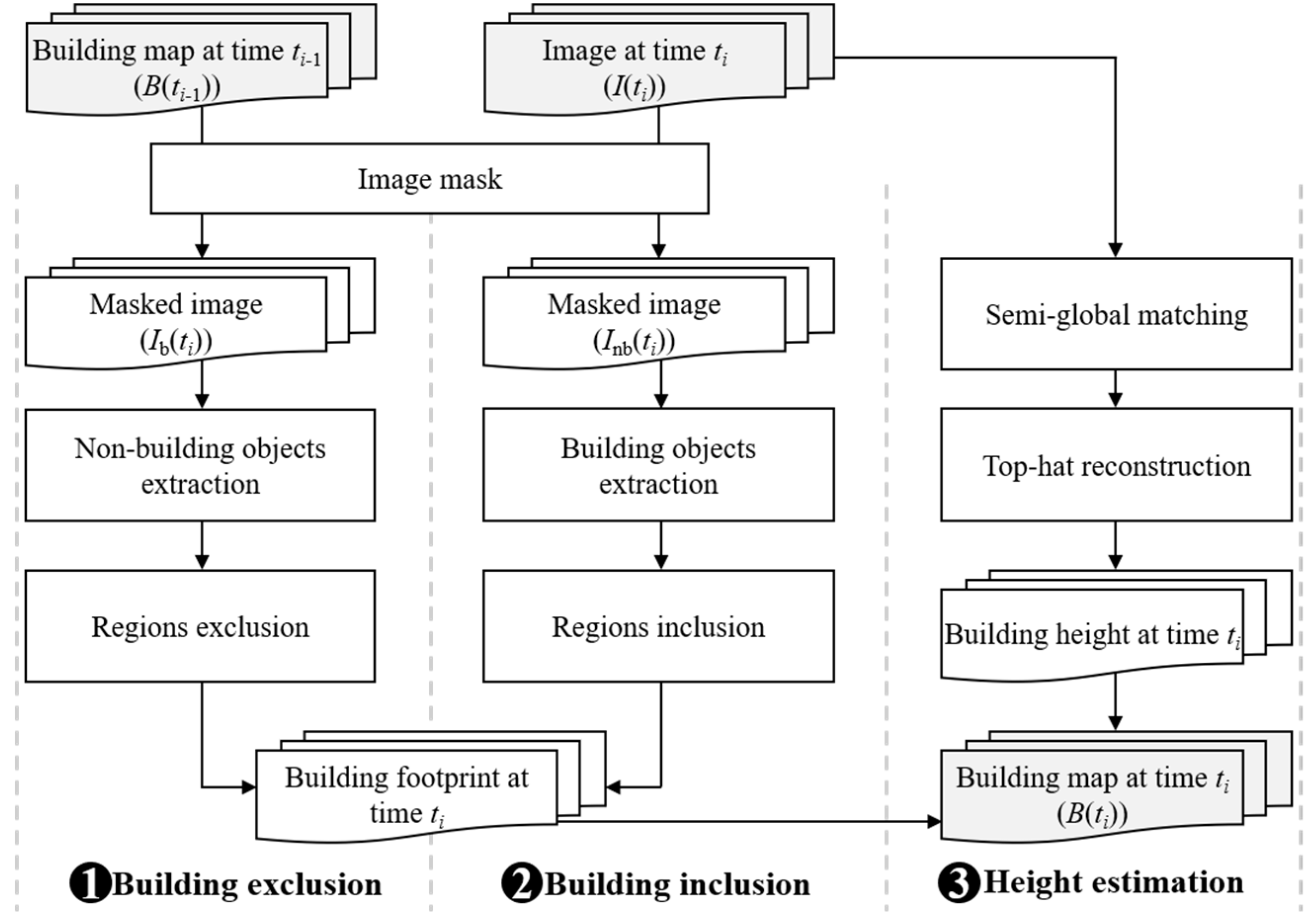
2.2. Generation of Time-Series 3D Building Maps

The time-series 3D building maps and their corresponding remote sensing images were denoted as B(t_i) and I(t_i) (i = 1, 2, …, n), respectively, and the pre-existing 3D building maps from Amap were denoted as B(t₀). The basic idea of generating B(t_i) (i = 1, 2, …, n) is considering B(t_i−1) as the base layer and updating the temporally inconsistent building footprints through image-to-map (i.e., I(t_i) to B(t_i−1)) change detection, and then estimating the height of the newly constructed buildings. The basic idea of image-to-map change detection is detecting building and non-building objects from I(t_i) in the non-building and building regions of B(t_i−1), respectively, which can avoid unnecessary computation and minimize false alarms [52]. The procedure of generating time-series 3D building maps (including footprint and height for each building) consists of three steps: 1) building exclusion; 2) building inclusion; and 3) height estimation (Figure 3).

2.2.1. Building Exclusion

In “building exclusion”, objects that are building and non-building in B(t_i−1) and I(t_i) respectively are detected, and their labels are updated as building in B(t_i). In this step, as non-building regions in B(t_i−1) are not of interest and can be removed, the corresponding regions in I(t_i) were masked out and a masked image I_b(t_i) was obtained. Non-building objects extraction based on I_b(t_i) was then conducted to locate the transition from building in B(t_i−1) to non-building in I(t_i). In this research, an unsupervised clustering method was developed to extract non-building objects. Since non-building pixels that changed from building ones in a short time period, i.e., about one year, mainly refer to vegetation and bare soil in urban areas, features that are relevant to vegetation and bare soil were considered. It should be noted that non-building pixels can be roads, parking lots, water, etc., but for this study vegetation and bare soil was the predominate case of non-building.

(1) NDVI (normalized difference vegetation index). The NDVI, normalized difference of near-infrared and red bands, can be used to differentiate vegetation and non-vegetation [53]. A high NDVI value indicates a high probability of vegetation.

(2) HSV (hue, saturation, value). The HSV color space converted from RGB space quantitatively describes colors by hue, saturation, and luminance. Therefore, the HSV color space can be used to detect soil by selecting pixels with hue values of yellow, red, and brown. It should be noted that although some buildings can be spectrally similar to soil, the following steps of object-based processing, visual interpretation, and manual correction can help to reduce the false alarms.

K-means clustering (eight clusters) was applied to the stacked HSV-NDVI feature, to obtain a classification map (including vegetation, bare soil, and other classes). The “vegetation” and “bare soil” classes were manually labeled as “non-building” by comparing the classification result with image I_b(t_i). To reduce the salt-and-pepper noise in the pixel-wise result, object-based image analysis was adopted. Multi-scale segmentation was performed and the proportion of non-building pixels in each object was calculated. When the proportion of non-building pixels of an object exceeded 50%, it was identified as a non-building object. 50% threshold wad determined based on a majority criterion.

2.2.2. Building Inclusion

“Building inclusion” refers to detecting regions that are non-building in B(t_i−1) and building in I(t_i) and updating them as building in B(t_i). Likewise, regions in I(t_i) corresponding to building in B(t_i−1) were masked out, generating a masked image I_nb(t_i). Building objects extraction of I_nb(t_i) was conducted based on the multi-scale segmentation and morphological building index (MBI) [54]. MBI is a recently developed automatic building extraction method for high-resolution remote sensing imagery, which uses morphological operators to represent the implicit spectral-structural characteristics of buildings (i.e., brightness, local contrast, size, and isotropy) in high-resolution satellite imagery. Then the proportion of building pixels in each object was calculated. Objects with a proportion larger than 50% were labeled as building.

2.2.3. Building Height Estimation

The height estimation was only conducted for newly included buildings in B(t_i), since the height values of these buildings were not available in B(t_i−1). The building height was generated through stereo-photogrammetry of the ZY-3 multi-view images [55]. For the building height, the DSM was first generated by the commonly used semi-global matching (SGM) method [56]. Subsequently, the height values for the above-ground objects (e.g., buildings) were derived by removing the bare-earth terrain from the DSM through white top-hat by reconstruction [57]. When multi-view remote sensing images were not available, the GF-1 and GF-2 satellite data were used as an alternative to identify the demolished/constructed buildings and update their footprints, and the height of the constructed buildings was obtained from the ZY-3 images of the next year.

2.2.4. Accuracy Assessment

The quantitative accuracy of the 3D building maps was assessed from two aspects: footprint and height. For the accuracy assessment of building footprint, 250 random polygons for each category, i.e., building and non-building, (total of 500 samples) were chosen for each city in each year. Specifically, a large number of random sampling locations (e.g., 2000) were selected, and the corresponding polygons where the first 250 random building and non-building pixels located were manually digitalized and used for the accuracy assessment. The accuracy of the building footprints was assessed with an object-based approach, and two metrics—average difference of area (ADA) and average difference of shape index (ADSI)—were used to depict the accuracy of the footprints [58]. In addition, overall accuracy (OA), user’s accuracy (UA), and producer’s accuracy (PA)were employed [59]. In order to test whether statistical difference in accuracies between time-series groups was significant, one-way analysis of variance (ANOVA) was conducted with a 95% confidence level (p < 0.05). With respect to the accuracy assessment of building height, around 100 sampled buildings were used as reference for each city. Due to the lack of ground-truth data, the reference building height was collected by counting the numbers of floors (the floor height being 3 m) using Baidu street view maps [60,61].

For accuracy assessment of the building change trajectory, 100 randomly selected sample points within changed regions were selected for each city. The reference trajectories were collected via visual inspection of the time-series high-resolution satellite imagery. For each sample, only when its labels (i.e., building or non-building) were always consistent between the mapping and reference trajectories was it considered a correctly mapped one. The correctness of the building change trajectory was calculated as the ratio of the number of pixels with correct trajectories to the total number of sample points.

2.3. Analyzing 3D Building Change and Urban Redevelopment Patterns

In order to characterize the 3D building change and urban redevelopment patterns, change characteristics of size, height, volume and span of individual buildings, building density in urban function zones, overall metrics over the study areas, and spatial autocorrelation of building density metrics were analyzed (

Table 2. The definitions of the 2D/3D parameters used in the study.

Abbreviation	Definition
Individual building level
Building size (BS)	ai
Building span (BD)	min(dist(i,j),j = 1,2,…,n)
Building height (BH)	hi
Building volume (BV)	ai × hi
Local neighborhood
Building coverage ratio (BCR)	$\frac{{{\displaystyle \sum }}_{i = 1}^M{a}_i}{S_L}$
Floor area ratio (FAR)	$\frac{{{\displaystyle \sum }}_{i = 1}^M{a}_i\times h_i/h_{floor}}{S_L}$
Urban functional zones
Building coverage ratio (BCR)	$\frac{{{\displaystyle \sum }}_{i = 1}^M{\mathrm{a}}_i}{S_{block}}$
Floor area ratio (FAR)	$\frac{{{\displaystyle \sum }}_{i = 1}^M{a}_i\times h_i/h_{floor}}{S_{block}}$
Entire study area
Total building coverage (COV)	${{\displaystyle \sum }}_{i = 1}^M{a}_i$
Area-weighted average height (H_W)	$\frac{{{\displaystyle \sum }}_{i = 1}^M{a}_i\times h_i}{{{\displaystyle \sum }}_{i = 1}^M{a}_i}$
Percent of the number (P_Num)	$\frac{Num\left(j\right)}{{{\displaystyle \sum }}_{j = 1}^{4}Num\left(\mathrm{j}\right)}$
Percent of the coverage (P_C)	$\frac{Cov\left(j\right)}{{{\displaystyle \sum }}_{j = 1}^{4}Cov\left(\mathrm{j}\right)}$
Floor area ratio (FAR)	$\frac{{{\displaystyle \sum }}_{i = 1}^M{a}_i\times h_i/h_{floor}}{S}$
Where ai and hi is the size and height of the ith building, respectively, dist(i,j) is the minimum span between the ith and jth buildings, M is the total number of buildings in area of interest, SL, Sblock, and S is the size of local neighborhood, block and study area, respectively, hfloor is the floor height, Num and Cov is the number and coverage for the low/mid/high/very high-rise buildings

).

2.3.1. Overall Change Analysis

In order to analyze the general trend of the 3D building change and redevelopment patterns, the following parameters were considered: total building coverage (COV), area-weighted average height (H_W), floor area ratio (FAR), percentage of the number for the low/mid/high/very high-rise buildings (P_Num), and percentage of the coverage for the low/mid/high/very high-rise buildings (P_C) (Table 2). Time-series COV, H_W, and FAR can indicate overall change in the horizontal direction, vertical direction, and 3D space, respectively. P_Num and P_C were used to reflect the composition of vertical structures at different height levels in terms of number and coverage. The buildings were categorized as four classes: low-rise (<10 m), mid-rise (10–24 m), high-rise (24–90 m), and very high-rise (>90 m) buildings, according to the Chinese Code for Design of Civil Buildings (http://www.zzguifan.com/webarbs/book/404/1476906.shtml) [62].

2.3.2. Change Analysis of Individual Buildings

To characterize the change at the level of individual buildings, the parameters of individual buildings were considered, referring to height (BH), footprint size (BS), volume (BV), and building span (BD) (See Table 2). BS, BH, and BV are the basic geometric attributes for each building. BD, i.e., the distance between the nearest buildings, is also an important parameter related to the sunshine hours, lighting, ventilation, sound insulation, and so on [63]. Taking advantage of the time-series high-resolution 3D building maps, a linear regression between time and mean building parameters (i.e., BH, BS, BV, and BD) was conducted separately for each city. The slope of this regression was considered as the annual change rate. In addition, the parameters of the constructed and demolished buildings were compared, in order to investigate the urban redevelopment patterns.

2.3.3. Development of Urban Functional Zones

Urban functional zones (UFZs), such as residential, commercial, industrial, urban green space, public service, agricultural, open space, etc. (

Table 3. Description of urban functional zones (UFZs).

UFZs	Description
Residential area	urban villages, apartments, residential buildings, shantytowns, etc.
Commercial area	shopping malls, banks, hotels, restaurants, supermarkets, etc.
Industrial area	factories, warehouses, high-tech industrial buildings, etc.
Urban green space	parks, forest, gardens etc.
Public service	government buildings, hospitals, schools, research institutes, etc.
Agricultural area	farmland, aquaculture ponds, etc.
Open space	undeveloped areas, under-construction sites, etc.

), provide different social, economic, and ecological functions, such as dwelling, commerce, landscaping, and industry [64]. Since UFZs are the basic units of urban planning and management in China, 3D urban redevelopment of the UFZs is of great concern. In this research, the UFZ types were mainly identified through visual interpretation of the high-resolution remote sensing data since they vary in terms of land cover composition and spatial variability. In addition, point of interest data in online map that providing names of restaurants, hotels, banks, hospitals, communities, companies, etc., and Baidu street view map were used to further validate its type. The building density (BCR and FAR) at the UFZ level was analyzed to reveal its change characteristics.

2.3.4. Spatiotemporal Pattern of the Local Neighborhood

BCR and FAR were calculated within a grid cell (local neighborhood). BCR [65], the ratio of the building coverage area to the size of the local neighborhood, depicts the two-dimensional building density in each grid cell. FAR [65], the ratio of the gross building floor area to the size of the local neighborhood, measures the 3D building density in each grid cell. A larger FAR signifies a higher land-use intensity [66].

To explore the spatiotemporal patterns of the 2D/3D building density, the global Moran’s I statistic [67] and the Getis-Ord Gi* spatial statistic [68] were adopted to measure the spatial autocorrelation from 2012 to 2017. The global Moran’s I statistic, a global spatial autocorrelation measure, ranges from −1 to 1. Moran’s I values that are close to 0, −1, and 1 indicate a spatially random, dispersed, and clustered distribution of a variable (here referring to BCR and FAR), respectively. To investigate the global autocorrelation bias at multiple spatial scales, the global Moran’s I analysis with four different neighborhood sizes, i.e., 100 m, 200 m, 500 m, and 1000 m was conducted. The Getis-Ord Gi* statistical analysis, a method measuring the degree of local autocorrelation of a variable, was used to identify statistically significant aggregations of low values (coldspots) and high values (hotspots). The output of the Getis-Ord Gi* statistical analysis, i.e., the GiZscore, is indicative of the degree of spatial autocorrelation. Values of GiZscore > 2.58, 1.96 < GiZscore < 2.58, and 1.65 < GiZscore < 1.96 indicate hotspots with 99%, 95%, and 90% confidence levels, respectively. Values of GiZscore < −2.58, −2.58 < GiZscore < −1.96, and −1.96 < GiZscore < −1.65 indicate coldspots with 99%, 95%, and 90% confidence levels, respectively.

3. Results and Discussion

3.1. Accuracy Assessment of the Time-Series 3D Building Maps

An example of a 2D image and the corresponding 3D building map is shown in Figure 4 for a visual inspection, from which it can be observed that the height distinction between buildings and ground objects (such as rivers and roads) is apparent. In addition, different buildings such as skyscrapers, malls, residential houses, and office buildings are effectively demonstrated in the 3D urban data. A quantitative accuracy assessment of the time-series 3D building maps was also conducted. On the one hand, 3D data represent both planar and vertical directions. On the other hand, for time-series results, change trajectories need to be evaluated. Therefore, evaluation of the time-series 3D building data in our research was conducted through the following ways: 1) quantitative assessment of the 3D building maps (footprint and height) for each year and 2) quantitative assessment of the time-series building change trajectories.

3.1.1. Quantitative Assessment of the 3D Building Maps

The object-based accuracy assessment of the building footprints of the time-series 3D building data of the four cities is presented in

Table 4. Accuracy assessment of the building footprints of the 3D building data (OA = overall accuracy, ADA = average difference of area, ADSI = average difference of shape index).

Data	OA (%)	ADA (%)	ADSI (%)
Beijing 2012	93.80	9.12	4.52
Beijing 2013	95.00	10.82	3.48
Beijing 2014	96.80	12.23	4.14
Beijing 2015	96.00	10.67	4.83
Beijing 2016	96.00	9.69	3.18
Beijing 2017	95.20	9.33	3.86
Xi’an 2012	87.68	8.63	3.88
Xi’an 2013	90.91	16.40	5.04
Xi’an 2015	89.37	8.59	3.98
Xi’an 2016	84.84	10.40	4.30
Xi’an 2017	88.16	10.06	3.51
Shanghai 2012	96.00	10.24	3.65
Shanghai 2013	97.60	6.41	2.23
Shanghai 2014	97.00	9.13	2.35
Shanghai 2015	95.60	8.48	2.64
Shanghai 2016	93.60	8.77	4.32
Shanghai 2017	96.20	7.63	2.88
Wuhan 2012	97.00	7.45	7.40
Wuhan 2013	94.40	8.66	7.22
Wuhan 2015	93.20	8.89	7.59
Wuhan 2016	94.80	11.67	6.67
Wuhan 2017	92.20	10.04	6.36

. The results are satisfactory for all four cities over the years, with the overall accuracy ranging from 84.84% to 97.60%. The producer’s and user’s accuracies of the building footprints are larger than 90% in most cases. The ADA and ADSI values are around 10% and 5%, respectively, for the extracted building objects. Therefore, it is stated that the extracted building objects show good agreement in size and shape with the reference samples. The ANOVA test results indicate that there are no statistical differences of accuracies between time-series groups (p = 0.78, 0.81, and 0.92 for OA, ADA, and ADSI, respectively).

Strong correlation (R2 > 0.9) between the estimated and reference building height values can be observed (

Table 5. Height estimation accuracy of the 3D building data (RMSE = root-mean-square error).

	Beijing	Xi’an	Shanghai	Wuhan
RMSE (m)	7.31	4.94	5.49	6.55
Slope	1.10	1.05	1.03	0.93
Bias (m)	−0.49	0.02	−0.14	2.30
R2	0.92	0.93	0.92	0.94

). In addition, the linear fit yields slope values ranging from 0.93 to 1.10, and bias values close to zero. It can therefore be said that the generated 3D building data show good agreement with the reference height. The RMSEs are 7.31 m, 4.94 m, 5.49 m, and 6.55 m, respectively, for the results of Beijing, Xi’an, Shanghai, and Wuhan.

3.1.2. Quantitative Assessment of the Building Change Trajectory

Correctness levels of 82.00%, 78.00%, 86.00%, and 86.00% were achieved for Beijing, Xi’an, Shanghai, and Wuhan, respectively. In a one-year tolerance strategy [69], when mapping and reference trajectory are only inconsistent for one year, it is still considered to be correctly mapped. After the one-year tolerance strategy was adopted, the correctness for Beijing, Xi’an, Shanghai, and Wuhan was improved to 93.00%, 92.00%, 94.00%, and 93.00%, respectively.

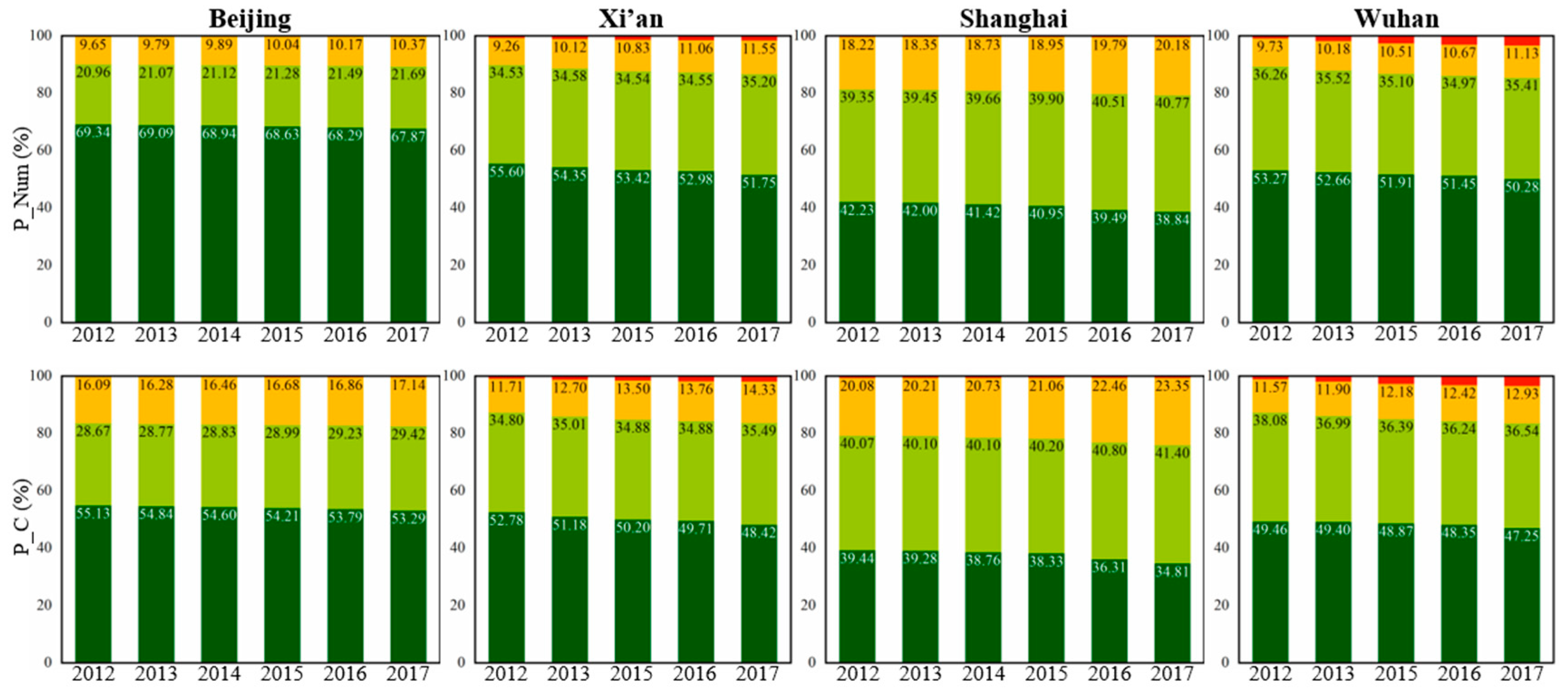
3.2. Overall Change Analysis

As can be seen in Figure 5, a general decreasing trend of total building coverage (COV) can be observed in inner-city areas for all the cities. Meanwhile, the area-weighted average height (H_W) showed a gradually increasing trend over the study period. In addition, a general increase in FAR is indicated by

Table 6. Floor area ratio (FAR) of the inner-city areas of the four Chinese megacities during 2012–2017.

City	Year	FAR
Beijing	2012	1.09
	2013	1.10
	2014	1.11
	2015	1.11
	2016	1.11
	2017	1.11
Xi’an	2012	1.16
	2013	1.22
	2015	1.28
	2016	1.32
	2017	1.31
Shanghai	2012	1.13
	2013	1.13
	2014	1.14
	2015	1.15
	2016	1.15
	2017	1.13
Wuhan	2012	0.63
	2013	0.64
	2015	0.65
	2016	0.66
	2017	0.67

, which reveals that the land-use efficiency of the inner-city areas has been improved through the urban redevelopment. It should be noted that the study areas of our research, i.e., the inner-city areas of the four Chinese megacities, do not cover urban fringes or rural areas. Our results show, quantitatively, for the first time, that the total building coverage has decreased, accompanied by an increase in both area-weighted height and FAR in the inner-city areas of the Chinese megacities, due to urban redevelopment. The decrease of COV further demonstrates that building coverage has tended to decrease in the inner-city areas. The transformation of old villages, factories, and neighborhoods has been the focus of urban redevelopment in China [70,71], most of which are compact low-rise buildings. In order to maximize land profit and satisfy the ever-increasing demand for housing space, taller buildings are being constructed in the available land [72]. Although construction of these dense high-rise buildings can maximize land-use efficiency, there is a requirement to maximize the space between buildings to improve the environment (air penetration, solar radiation, day lighting, and air temperature) [73]. Against this background, compact low-rise buildings are usually replaced with open high-rise buildings in urban redevelopment, leading to a decrease of the total building coverage in the inner-city areas.

Additionally, as shown in Figure 6, for low-rise buildings in all four megacities, their number and coverage (P_Num/P_C) declined slightly from 2012 to 2017. The number and coverage for high and very high-rise buildings showed a steady increase, especially for very high-rise buildings in Xi’an and Wuhan, where the P_Num and P_C values nearly doubled over the five years. The increase of high-rise and very high-rise buildings and the decrease of low-rise buildings further demonstrates that the inner-city areas of Chinese megacities have witnessed vertical development to tackle the land scarcity problem [65].

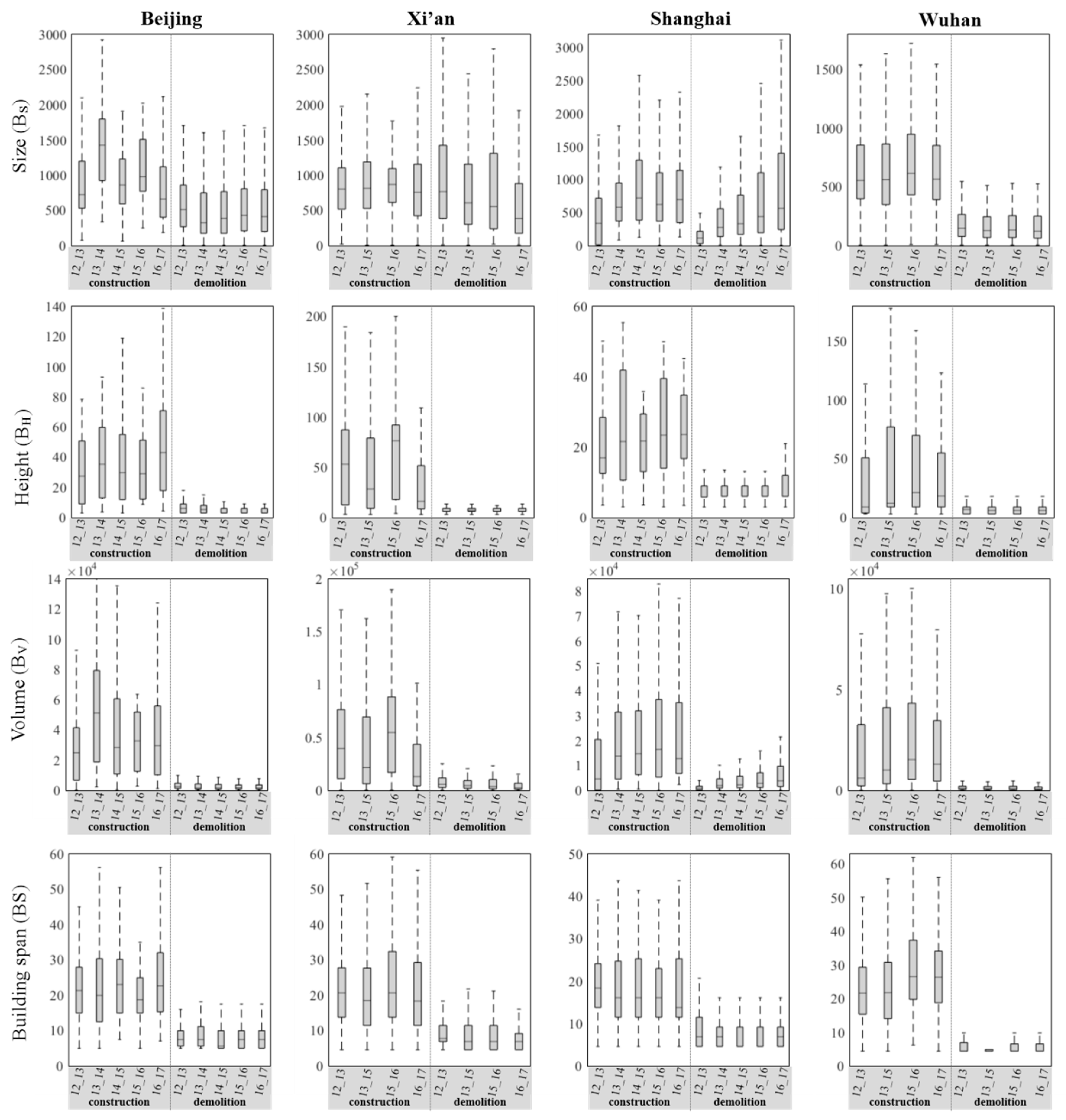
3.3. Change of Iindividual Buildings

The annual change rates of the mean values of building size, height, volume, and span are presented in

Table 7. Annual change rate of the average values of the basic building attributes, i.e., building size, height, volume, and span (p < 0.05).

	Size (m2/year)	Height (m/year)	Volume (m3/year)	Span (m/year)
Beijing	1.89*	0.09*	121.86*	0.04*
Xi’an	−0.87	0.42*	409.93*	0.12*
Shanghai	−0.95	0.18*	165.52	0.10*
Wuhan	5.48*	0.24*	208.68*	0.17*

. In general, all four cities have showed an increase of average building size, height, volume, and span during the period 2012–2017 at a 95% confidence level (p < 0.05). However, a decreased trend is found for average building height in both Xi’an and Shanghai, which is not significant at the 0.05 level. In addition, there is a nonsignificant increment, i.e., 165.52 m³·year⁻¹, for the average building volume in Shanghai. Significant rates are obtained for the three other cities, i.e., 121.86 m³·year⁻¹ for Beijing, 409.93 m³·year⁻¹ for Xi’an, and 208.68 m³·year⁻¹ for Wuhan. The significant annual change rates of the average building size are 1.89 and 5.48 m²·year⁻¹ for Beijing and Shanghai, respectively. For the average building height/span, their significant annual change rates are 0.11/0.05, 0.42/0.12, 0.18/0.10, and 0.24/0.17 m·year⁻¹ for Beijing, Xi’an, Shanghai, and Wuhan, respectively.

It is further revealed that the constructed and demolished buildings exhibit strikingly distinct characteristics (Figure 7). Compared to the demolished buildings, the constructed ones tend to have a significantly larger height, volume, and span for all the study areas throughout the whole period, which validates the finding that compact low-rise buildings have been replaced by open high-rise ones in the urban redevelopment. With regard to the building size, Beijing and Wuhan have larger values for constructed buildings compared to demolished ones, but no significant differences were found for Xi’an and Shanghai.

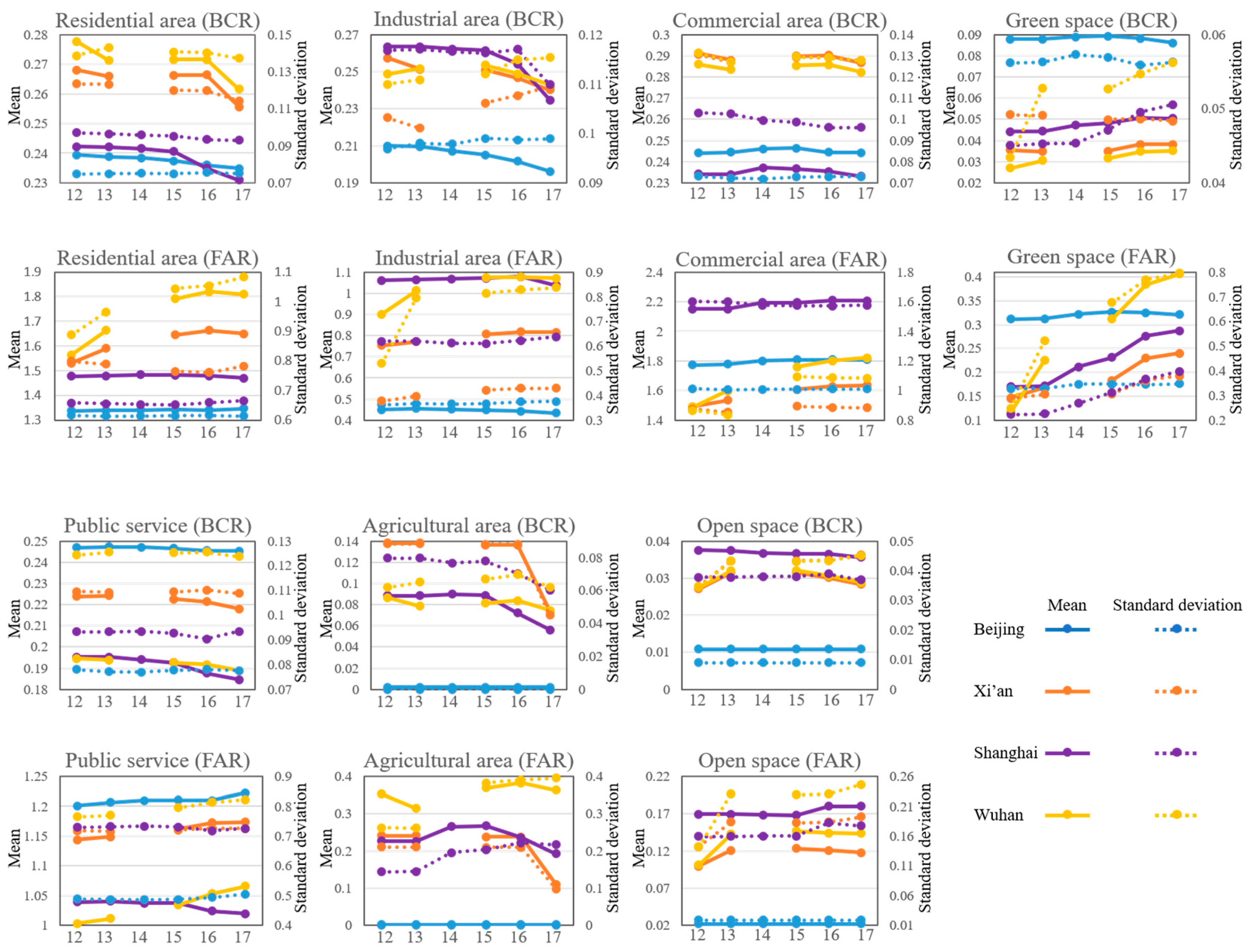
3.4. Change Analysis of the Urban Functional Zones

Change analysis of the UFZs was conducted by calculating the time-series mean and standard deviation of building density (BCR and FAR) in all the blocks of a certain type of UFZ (Figure 8). The mean and standard deviation indicate the average and variation of the building density.

As indicated by the time-series mean values, decreasing and increasing trends can be observed for BCR and FAR, respectively, which is partly due to the replacement of compact low-rise building areas with open high-rise ones (Figure 9a), as mentioned in Section 3.2 and Section 3.3. Meanwhile, urban redevelopment has been dedicated to optimizing land-use structure, in order to mitigate the “big city diseases” [74]. For example, as shown in Figure 9b,d, areas with high building density have been redeveloped to urban green spaces, leading to an inevitable decrease of BCR and a possible increase of FAR. The three main UFZs, i.e., residential, industrial, and commercial areas, have similar ranges of mean BCR. The commercial area has the largest mean FAR, followed by the residential and industrial areas. For mean BCR in the industrial area of Shanghai, the turning point from stable to decreasing trend occurred in 2015. However, its mean FAR decreased as well, which contradicts the general increasing trend of FAR. It is found that the old industrial areas have been either relocated or updated, as shown in Figure 9c,b, in order to improve the environment in the densely populated areas [75]. For the four other UFZs, only green spaces witnessed an increase in both BCR and FAR.

Comparing the standard deviations of BCR and FAR, it can be seen that the variation of FAR is much higher than that of BCR. In general, the values of standard deviation have shown an increasing tendency in the different UFZs, showing that the urban redevelopment has led to a greater variation of 3D building density. However, no general trend can be observed for the variation of BCR.

3.5. Spatiotemporal Patterns of the Local Neighborhoods

3.5.1. Global Pattern Analysis

(Figure 10). The BCR and FAR of all the cities exhibit positive spatial correlation at a 99% significance level, revealing the clustered spatial pattern of both local 2D and 3D building density. In addition, with a larger neighborhood size, stronger spatial autocorrelation is found, as indicated by the increase of the Moran’s I index value. However, the Moran’s index values at the neighborhood size of 1000 m are only slightly larger than those for a neighborhood size of 500 m. Considering that more spatial details can be captured at smaller scales, the neighborhood size of 500 m was chosen.

All four cities witnessed a variation of the Moran’s I index value for both BCR and FAR in terms of temporal change, as shown in Figure 11. In general, most Moran’s I values for BCR showed an increasing trend, except for Wuhan, indicating that the spatial autocorrelation of the 2D building density has grown with the urban redevelopment. The Moran’s I values of FAR remained relatively stable in Beijing and Shanghai, and became smaller in Xi’an and Wuhan.

3.5.2. Local Spatiotemporal Pattern Analysis

To characterize the local spatiotemporal patterns of building density, the GiZscore maps for the years 2012 and 2017, the temporal change of hotspots and coldspots, and the number of hotspots and coldspots are presented in Figure 12a–c, respectively. Firstly, BCR-FAR hotspots/coldspots are identified as the spatially overlapped regions of BCR and FAR hotspots/coldspots. In most cities, except for Beijing, 60.23%–65.48% BCR hotspots and 42.39%–68.88% FAR hotspots are found to be BCR-FAR hotspots. 71.21%–81.85% BCR coldspots and 52.96%–75.67% FAR coldspots are BCR-FAR coldspots in the four cities. This signifies that most neighborhoods show statistically significant aggregation of high/low building density values in both 2D and 3D space. However, the spatial distribution of the BCR and FAR hotspots/coldspots is different. Overall, coldspots show a more scattered pattern, and are mostly located away from the urban centers. Hotspots for both BCR and FAR can be seen to have a spatial agglomeration pattern, forming a series of spatially contiguous regions (marked by the oval in Figure 12A). BCR hotspots mainly locate in the urban core areas, such as Dongcheng District and Xicheng District of Beijing (Figure 12a1), and Huangpu District of Shanghai (Figure 12e1). FAR hotspots are mainly located in the business districts, such as Xi’dan of Beijing (Figure 12b1), Zhonglou of Xi’an (Figure 12d2), Lujiazui of Shanghai (Figure 12f2), and Hanzheng Street of Wuhan (Figure 12h1).

The spatial change of these spatially contiguous regions was analyzed by comparing the GiZscore maps of 2012 and 2017 (Figure 12A). Regions of BCR hotspots with a larger area, such as Figure 12a1,c2,e1,g2, have spatially expanded, and regions of BCR hotspots with a smaller area, such as Figure 12a2,e2,e3,e4,g1,g3,g4, have tended to shrink. In addition, regions of FAR hotspots with a larger area, such as Figure 12b1,d2,f1,h1,h2, have spatially shrunk. Furthermore, the temporal change of the hotspots and coldspots was analyzed by categorizing them as: (1) consecutive hotspots, i.e., hotspots through all the years; (2) consecutive coldspots, i.e., coldspots through all the years; (3) change from coldspots to hotspots over adjacent two-year periods; (4) change from hotspots to coldspots over adjacent two-year periods; (5) change from coldspots in 2012 to hotspots in 2017; and (6) change from hotspots in 2012 to coldspots in 2017 (Figure 12B). In general, only persistent hotspots and coldspots were found for all the cities, and no transition between hotspots and coldspots was observed over the time span of one year. Therefore, it can be concluded that the local patterns of urban redevelopment are unlikely to shift between hotspots and coldspots over a short time period, and urban redevelopment activities (building construction or demolition) tend to show a scattered spatial distribution in the inner-city areas. Meanwhile, a change from hotspots in 2012 to coldspots in 2017 only occurred in Shanghai, due to the very large scale (8.31 km²) demolition of urban villages in Sanlin and Pudong (Figure 12e3).

The temporal variation of the number of hotspots and coldspots during 2012–2017 is depicted in Figure 12C. The numbers of BCR hotspots, BCR coldspots, FAR hotspots, and FAR coldspots have generally changed only slightly. A notable increase in the number can only be observed for the BCR hotspots and coldspots of Shanghai during 2015–2017.

4. Conclusions

With the establishment of boundary “red lines” for urban growth and the conservation of basic farmland and ecological land, the contradiction between the supply and demand for land in Chinese cities has become predominant, especially in the inner-city areas [76] (Yan et al., 2015). In the meantime, unsustainable urban development has caused a series of problems, such as low-efficiency land use or even land vacancy, which have further hampered the socioeconomic development of Chinese cities [77]. Therefore, the transformation from new land development to stock land redevelopment has become an inevitable trend in Chinese megacities.

In this paper, a framework for generating time-series 3D building maps by the use of time-series multi-view ZY-3 satellite imagery has been presented. A map-to-image comparison strategy by integrating prior building, spectral, structural, and multi-view information was developed to generate footprint and height information for each building. This framework was applied in the inner-city areas of the four representative Chinese megacities—Beijing, Xi’an, Shanghai, and Wuhan—in order to analyze the 3D building change and urban redevelopment patterns. The experimental results showed that the proposed method can generate satisfactory time-series 3D building maps with an overall accuracy of 84.84%–97.60%, a height estimation error of 4.94–7.31 m, and a building change trajectory correctness of around 85%. Based on the time-series results, the 3D inner-city redevelopment patterns were analyzed at the level of the entire study area, individual buildings, the local neighborhood, and UFZs:

(1)

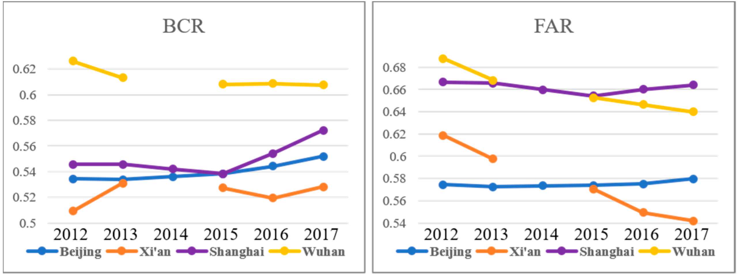
In all the study areas, a decrease in the total building coverage and an increase in both the area-weighted building height and FAR were found.

(2)

By investigating the change of individual buildings, a significant increase of the average building height and span was observed, indicating replacement of compact low-rise buildings with open high-rise buildings in the inner-city redevelopment.

(3)

There has been a general reduction and increment of the mean BCR and FAR, respectively, in most of the UFZs, due to the fact that inner-city redevelopment has been dedicated to improving land-use efficiency and optimizing land-use structure.

(4)

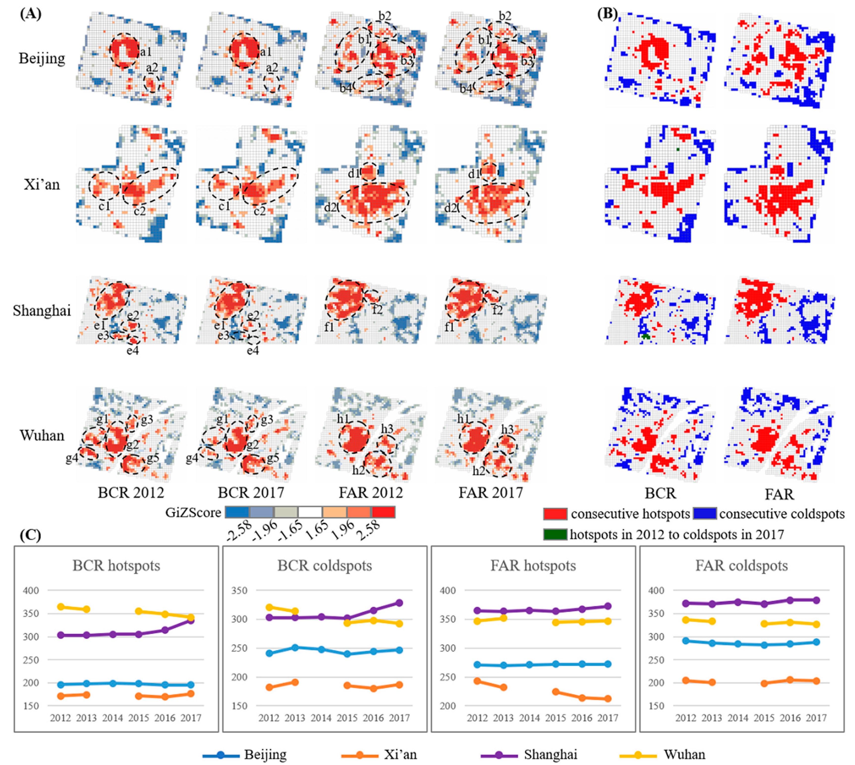
Based on the global and local spatial autocorrelation of the 2D and 3D building density (BCR and FAR), since urban redevelopment has taken place in scattered locations in the inner-city areas, the local patterns are unlikely to shift between hotspots and coldspots over the short time period.

References

1. Xinhua. China’s Urbanization Plan 2014–2020. 2014. Available online: http://www.chinadaily.com.cn/business/2014-03/18/content_17355936_2.htm (accessed on 18 March 2014).
2. Zhang, S.; Zhang, X. Analysis of Urban Expansion Process Based on GIS and RS in Suihua. In Proceedings of the International Conference on Information Engineering and Computer Science (ICIECS), Wuhan, China, 25–26 December 2010; pp. 1–4. [Google Scholar]
3. Song, W.; Liu, M. Farmland conversion decreases regional and national land quality in China. Land Degrad. Dev. 2017, 28, 459–471. [Google Scholar] [CrossRef]
4. Xie, C.; Huang, X.; Mu, H.; Yin, W. Impacts of land-use changes on the lakes across the Yangtze floodplain in China. Environ. Sci. Technol. 2017, 51, 3669–3677. [Google Scholar] [CrossRef] [PubMed]
5. Huang, H.; Chen, Y.; Clinton, N.; Wang, J.; Wang, X.; Liu, C.; Gong, P.; Yang, J.; Bai, Y.; Zheng, Y. Mapping major land cover dynamics in Beijing using all Landsat images in Google Earth Engine. Remote Sens. Environ. 2017, 202, 166–176. [Google Scholar] [CrossRef]
6. Lü, Y.; Zhang, L.; Feng, X.; Zeng, Y.; Fu, B.; Yao, X.; Li, J.; Wu, B. Recent ecological transitions in China: Greening, browning, and influential factors. Sci. Rep. 2015, 5, 8732. [Google Scholar] [CrossRef]
7. He, C.; Liu, Z.; Xu, M.; Ma, Q.; Dou, Y. Urban expansion brought stress to food security in China: Evidence from decreased cropland net primary productivity. Sci. Total Environ. 2017, 576, 660–670. [Google Scholar] [CrossRef] [PubMed]
8. Liu, F.; Zhang, Z.; Zhao, X.; Wang, X.; Zuo, L.; Wen, Q.; Yi, L.; Xu, J.; Hu, S.; Liu, B. Chinese cropland losses due to urban expansion in the past four decades. Sci. Total Environ. 2019, 650, 847–857. [Google Scholar] [CrossRef] [PubMed]
9. Huang, X.; Cai, Y.; Li, J. Evidence of the mitigated urban particulate matter island (UPI) effect in China during 2000–2015. Sci. Total Environ. 2019, 660, 1327–1337. [Google Scholar] [CrossRef]
10. Yang, Q.; Huang, X.; Tang, Q. The footprint of urban heat island effect in 302 Chinese cities: Temporal trends and associated factors. Sci. Total Environ. 2019, 655, 652–662. [Google Scholar] [CrossRef]
11. Hong, W.; Yang, C.; Chen, L.; Zhang, F.; Shen, S.; Guo, R. Ecological control line: A decade of exploration and an innovative path of ecological land management for megacities in China. J. Environ. Manag. 2017, 191, 116–125. [Google Scholar] [CrossRef] [PubMed]
12. Zeuthen, J.W. Whose urban development? Changing credibilities, forms and functions of urbanization in Chengdu, China. Land Use Plan. 2017, 79, 942–951. [Google Scholar] [CrossRef]
13. Zheng, B.; Liu, G.; Wang, H.; Cheng, Y.; Lu, Z.; Liu, H.; Zhu, X.; Wang, M.; Yi, L. Study on the delimitation of the urban development boundary in a special economic zone: A case study of the central urban area of Doumen in Zhuhai, China. Sustainability 2018, 10, 756. [Google Scholar] [CrossRef]
14. Xinhua. Beijing-Tianjin-Hebei Coordinated Development Guideline Approved. 2015. Available online: http://en.people.cn/business/n/2015/0430/c90778-8886203.html (accessed on 30 April 2015).
15. Ni, P.; Kamiya, M.; Ding, R. Global Urban Competitiveness: Comparative Analysis from Different Perspectives. In Cities Network Along the Silk Road; Springer: Singapore, 2017; pp. 51–64. [Google Scholar]
16. Qian, C. How Shanghai Will Become a World-Class City by 2035. 2018. Available online: https://archive.shine.cn/metro/society/How-Shanghai-will-become-a-worldclass-city-by-2035/shdaily.shtml (accessed on 5 Janurary 2018).
17. Zhang, Z.; Li, N.; Wang, X.; Liu, F.; Yang, L. A comparative study of urban expansion in Beijing, Tianjin and Tangshan from the 1970s to 2013. Remote Sens. 2016, 8, 496. [Google Scholar] [CrossRef]
18. Bagan, H.; Yamagata, Y. Landsat analysis of urban growth: How Tokyo became the world’s largest megacity during the last 40years. Remote Sens. Environ. 2012, 127, 210–222. [Google Scholar] [CrossRef]
19. Sexton, J.O.; Song, X.P.; Huang, C.; Channan, S.; Baker, M.E.; Townshend, J.R. Urban growth of the Washington, D.C.–Baltimore, MD metropolitan region from 1984 to 2010 by annual, Landsat-based estimates of impervious cover. Remote Sens. Environ. 2013, 129, 42–53. [Google Scholar] [CrossRef]
20. Zhang, Q.; Seto, K.C. Mapping urbanization dynamics at regional and global scales using multi-temporal DMSP/OLS nighttime light data. Remote Sens. Environ. 2011, 115, 2320–2329. [Google Scholar] [CrossRef]
21. Huang, X.; Schneider, A.; Friedl, M.A. Mapping sub-pixel urban expansion in China using MODIS and DMSP/OLS nighttime lights. Remote Sens. Environ. 2016, 175, 92–108. [Google Scholar] [CrossRef]
22. Kuang, W.; Liu, J.; Dong, J.; Chi, W.; Zhang, C. The rapid and massive urban and industrial land expansions in China between 1990 and 2010: A CLUD-based analysis of their trajectories, patterns, and drivers. Landsc. Urban Plan. 2016, 145, 21–33. [Google Scholar] [CrossRef] [Green Version]
23. Xu, M.; He, C.; Liu, Z.; Dou, Y. How Did Urban Land Expand in China between 1992 and 2015? A Multi-Scale Landscape Analysis. PLoS ONE 2016, 11, e0154839. [Google Scholar] [CrossRef]
24. Mertes, C.M.; Schneider, A.; Sulla-Menashe, D.; Tatem, A.J.; Tan, B. Detecting change in urban areas at continental scales with MODIS data. Remote Sens. Environ. 2015, 158, 331–347. [Google Scholar] [CrossRef] [Green Version]
25. Ouyang, Z.; Fan, P.; Chen, J. Urban Built-up Areas in Transitional Economies of Southeast Asia: Spatial Extent and Dynamics. Remote Sens. 2016, 8, 819. [Google Scholar] [CrossRef]
26. Schneider, A.; Mertes, C.; Tatem, A.; Tan, B.; Sulla-Menashe, D.; Graves, S.; Patel, N.; Horton, J.; Gaughan, A.; Rollo, J. A new urban landscape in East–Southeast Asia, 2000–2010. Environ. Res. Lett. 2015, 10, 034002. [Google Scholar] [CrossRef] [Green Version]
27. Liu, X.; Hu, G.; Chen, Y.; Li, X.; Xu, X.; Li, S.; Pei, F.; Wang, S. High-resolution multi-temporal mapping of global urban land using Landsat images based on the Google Earth Engine Platform. Remote Sens. Environ. 2018, 209, 227–239. [Google Scholar] [CrossRef]
28. Angel, S.; Parent, J.; Civco, D.L.; Blei, A.; Potere, D. The dimensions of global urban expansion: Estimates and projections for all countries, 2000–2050. Prog. Plan. 2011, 75, 53–107. [Google Scholar] [CrossRef]
29. Frolking, S.; Milliman, T.; Seto, K.C.; Friedl, M.A. A global fingerprint of macro-scale changes in urban structure from 1999 to 2009. Environ. Res. Lett. 2013, 8, 024004. [Google Scholar] [CrossRef] [Green Version]
30. Wang, H.; Shen, Q.; Tang, B.S.; Lu, C.; Peng, Y.; Tang, L. A framework of decision-making factors and supporting information for facilitating sustainable site planning in urban renewal projects. Cities 2014, 40, 44–55. [Google Scholar] [CrossRef]
31. Shahtahmassebi, A.R.; Song, J.; Zheng, Q.; Blackburn, G.A.; Wang, K.; Huang, L.Y.; Pan, Y.; Moore, N.; Shahtahmassebi, G.; Sadrabadi Haghighi, R.; et al. Remote sensing of impervious surface growth: A framework for quantifying urban expansion and re-densification mechanisms. Int. J. Appl. Earth Obs. Geoinf. 2016, 46, 94–112. [Google Scholar] [CrossRef] [Green Version]
32. Zhang, T.; Huang, X. Monitoring of Urban Impervious Surfaces Using Time Series of High-Resolution Remote Sensing Images in Rapidly Urbanized Areas: A Case Study of Shenzhen. IEEE J. Sel. Top. Appl. Earth Obs. Remote Sens. 2018, 11, 2692–2708. [Google Scholar] [CrossRef]
33. Lefebvre, A.; Corpetti, T. Monitoring the morphological transformation of Beijing old city using remote sensing texture analysis. IEEE J. Sel. Top. Appl. Earth Obs. Remote Sens. 2017, 10, 539–548. [Google Scholar] [CrossRef]
34. Zambon, I.; Colantoni, A.; Salvati, L. Horizontal vs. vertical growth: Understanding latent patterns of urban expansion in large metropolitan regions. Sci. Total Environ. 2019, 654, 778–785. [Google Scholar] [CrossRef]
35. Zhang, W.; Li, W.; Zhang, C.; Ouimet, W.B. Detecting horizontal and vertical urban growth from medium resolution imagery and its relationships with major socioeconomic factors. Int. J. Remote Sens. 2017, 38, 3704–3734. [Google Scholar] [CrossRef]
36. Magnard, C.; Morsdorf, F.; Small, D.; Stilla, U.; Schaepman, M.E.; Meier, E. Single tree identification using airborne multibaseline SAR interferometry data. Remote Sens. Environ. 2016, 186, 567–580. [Google Scholar] [CrossRef]
37. Seong, J.C.; Park, T.H.; Ko, J.H.; Chang, S.I.; Kim, M.; Holt, J.B.; Mehdi, M.R. Modeling of road traffic noise and estimated human exposure in Fulton County, Georgia, USA. Environ. Int. 2011, 37, 1336–1341. [Google Scholar] [CrossRef]
38. Liu, C.; Huang, X.; Wen, D.; Chen, H.; Gong, J. Assessing the quality of building height extraction from ZiYuan-3 multi-view imagery. Remote Sens. Lett. 2017, 8, 907–916. [Google Scholar] [CrossRef]
39. Sampath, A.; Shan, J. Segmentation and reconstruction of polyhedral building roofs from aerial lidar point clouds. IEEE Trans. Geosci. Remote Sens. 2010, 48, 1554–1567. [Google Scholar] [CrossRef]
40. Ghosh, M.K.; Kumar, L.; Roy, C. Monitoring the coastline change of Hatiya Island in Bangladesh using remote sensing techniques. ISPRS J. Photogramm. Remote Sens. 2015, 101, 137–144. [Google Scholar] [CrossRef]
41. Jin, S.; Yang, L.; Zhu, Z.; Homer, C. A land cover change detection and classification protocol for updating Alaska NLCD 2001 to 2011. Remote Sens. Environ. 2017, 195, 44–55. [Google Scholar] [CrossRef]
42. Zhou, Y.; Smith, S.J.; Elvidge, C.D.; Zhao, K.; Thomson, A.; Imhoff, M. A cluster-based method to map urban area from DMSP/OLS nightlights. Remote Sens. Environ. 2014, 147, 173–185. [Google Scholar] [CrossRef]
43. Wang, S.; Tian, Y.; Zhou, Y.; Liu, W.; Lin, C. Fine-Scale Population Estimation by 3D Reconstruction of Urban Residential Buildings. Sensors 2016, 16, 1755. [Google Scholar] [CrossRef]
44. Qin, R. Rpc stereo processor (rsp)—A software package for digital surface model and orthophoto generation from satellite stereo imagery. ISPRS Ann. Photogramm. Remote Sens. Spat. Inf. Sci. 2016, 3, 77–82. [Google Scholar] [CrossRef]
45. Fang, C.; Yu, D.; Mao, H.; Bao, C.; Huang, J. Optimizing Measures and Policy Advices for the Spatial Pattern of China’s Urban Development. In China’s Urban Pattern; Springer: Singapore, 2018; pp. 283–311. [Google Scholar]
46. National Bureau of Statistics of China. China City Statistical Yearbook; China Statistics Press: Beijing, China, 2018. [Google Scholar]
47. Chang, Q.; Xu, Q.; Yang, C.; Wang, S. Reflections and Explorations on the Decremented Regulation of Construction Land in the New Beijing City Master Planning. China City Plan. Rev. 2018, 27, 25–35. [Google Scholar]
48. Long, X.; Bai, J.; Sun, Y. Western Chinese Urban Development Boundary Idea And Xi’an’s Practice. Planners 2016, 6, 003. [Google Scholar]
49. Fu, P.; Weng, Q. A time series analysis of urbanization induced land use and land cover change and its impact on land surface temperature with Landsat imagery. Remote Sens. Environ. 2016, 175, 205–214. [Google Scholar] [CrossRef]
50. Peng, J.; Liu, Y.; Ma, J.; Zhao, S. A new approach for urban-rural fringe identification: Integrating impervious surface area and spatial continuous wavelet transform. Landsc. Urban Plan. 2018, 175, 72–79. [Google Scholar] [CrossRef]
51. Radwan, T.M.; Blackburn, G.A.; Whyatt, J.D.; Atkinson, P.M. Dramatic Loss of Agricultural Land Due to Urban Expansion Threatens Food Security in the Nile Delta, Egypt. Remote Sens. 2019, 11, 332. [Google Scholar] [CrossRef]
52. Bouziani, M.; Goïta, K.; He, D.C. Automatic change detection of buildings in urban environment from very high spatial resolution images using existing geodatabase and prior knowledge. ISPRS J. Photogramm. Remote Sens. 2010, 65, 143–153. [Google Scholar] [CrossRef]
53. Townshend, J.R.; Justice, C. Analysis of the dynamics of African vegetation using the normalized difference vegetation index. Int. J. Remote Sens. 1986, 7, 1435–1445. [Google Scholar] [CrossRef]
54. Huang, X.; Zhang, L. Morphological building/shadow index for building extraction from high-resolution imagery over urban areas. IEEE J. Sel. Top. Appl. Earth Obs. Remote Sens. 2012, 5, 161–172. [Google Scholar] [CrossRef]
55. Qin, R. Change detection on LOD 2 building models with very high resolution spaceborne stereo imagery. ISPRS J. Photogramm. Remote Sens. 2014, 96, 179–192. [Google Scholar] [CrossRef]
56. Hirschmuller, H. Accurate and efficient stereo processing by semi-global matching and mutual information. In Proceedings of the IEEE Computer Society Conference on Computer Vision and Pattern Recognition, San Diego, CA, USA, 20–25 June 2005; pp. 807–814. [Google Scholar]
57. Qin, R.; Fang, W. A hierarchical building detection method for very high resolution remotely sensed images combined with DSM using graph cut optimization. Photogramm. Eng. Remote Sens. 2014, 80, 873–883. [Google Scholar] [CrossRef]
58. Doxani, G.; Karantzalos, K.; Tsakiri-Strati, M. Object-based building change detection from a single multispectral image and pre-existing geospatial information. Photogramm. Eng. Remote Sens. 2015, 81, 481–489. [Google Scholar] [CrossRef]
59. Nduati, E.; Sofue, Y.; Matniyaz, A.; Park, J.G.; Yang, W.; Kondoh, A. Cropland Mapping Using Fusion of Multi-Sensor Data in a Complex Urban/Peri-Urban Area. Remote Sens. 2019, 11, 207. [Google Scholar] [CrossRef]
60. Taubenböck, H.; Klotz, M.; Wurm, M.; Schmieder, J.; Wagner, B.; Wooster, M.; Esch, T.; Dech, S. Delineation of Central Business Districts in mega city regions using remotely sensed data. Remote Sens. Environ. 2013, 136, 386–401. [Google Scholar] [CrossRef]
61. Marcellus-Zamora, K.A.; Gallagher, P.M.; Spatari, S.; Tanikawa, H. Estimating materials stocked by land-use type in historic urban buildings using spatio-temporal analytical tools. J. Ind. Ecol. 2016, 20, 1025–1037. [Google Scholar] [CrossRef]
62. Blackman, I.; Picken, D.; Liu, C. Height and construction costs of residential buildings in Hong Kong and Shanghai. In Proceedings of the International Conference on Multi-National Construction Projects, Shanghai, China, 21–23 November 2008; pp. 1–18. [Google Scholar]
63. Wang, X.; Zhao, G.; He, C.; Wang, X.; Peng, W. Low-carbon neighborhood planning technology and indicator system. Renew. Sustain. Energy Rev. 2016, 57, 1066–1076. [Google Scholar] [CrossRef]
64. Yao, L.; Chen, L.; Wei, W.; Sun, R. Potential reduction in urban runoff by green spaces in Beijing: A scenario analysis. Urban For. Urban Green. 2015, 14, 300–308. [Google Scholar] [CrossRef] [Green Version]
65. Yu, B.; Liu, H.; Wu, J.; Hu, Y.; Zhang, L. Automated derivation of urban building density information using airborne LiDAR data and object-based method. Landsc. Urban Plan. 2010, 98, 210–219. [Google Scholar] [CrossRef]
66. Cai, H.; Wang, Z.; Zhang, Q. To build above the limit? Implementation of land use regulations in urban China. J. Urban Econ. 2017, 98, 223–233. [Google Scholar] [CrossRef]
67. Getis, A.; Ord, J.K. The analysis of spatial association by use of distance statistics. Geogr. Anal. 1992, 24, 189–206. [Google Scholar] [CrossRef]
68. Ord, J.K.; Getis, A. Local spatial autocorrelation statistics: Distributional issues and an application. Geogr. Anal. 1995, 27, 286–306. [Google Scholar] [CrossRef]
69. Song, X.P.; Sexton, J.O.; Huang, C.; Channan, S.; Townshend, J.R. Characterizing the magnitude, timing and duration of urban growth from time series of Landsat-based estimates of impervious cover. Remote Sens. Environ. 2016, 175, 1–13. [Google Scholar] [CrossRef]
70. Lin, G.C. The redevelopment of China’s construction land: Practising land property rights in cities through renewals. China Q. 2015, 224, 865–887. [Google Scholar] [CrossRef]
71. Wang, B.; Tian, L.; Yao, Z. Institutional uncertainty, fragmented urbanization and spatial lock-in of the peri-urban area of China: A case of industrial land redevelopment in Panyu. Land Use Policy 2018, 72, 241–249. [Google Scholar] [CrossRef]
72. Tao, J.; Wang, Q. Co-evolution: A Model for Renovation of Traditional Villages in the Urban Fringe of Guangzhou, China. J. Asian Archit. Build. Eng. 2014, 13, 555–562. [Google Scholar] [CrossRef] [Green Version]
73. Lau, S.S. Physical environment of tall residential buildings: The case of Hong Kong. In High-Rise Living in Asian Cities; Springer: Dordrecht, The Netherlands, 2011; pp. 25–47. [Google Scholar]
74. Bereitschaft, B. Gods of the city? Reflecting on city building games as an early introduction to urban systems. J. Geogr. 2016, 115, 51–60. [Google Scholar] [CrossRef]
75. Li, Y.; Chen, X.; Tang, B.S.; Wong, S.W. From project to policy: Adaptive reuse and urban industrial land restructuring in Guangzhou City, China. Cities 2018, 82, 68–76. [Google Scholar] [CrossRef]
76. Yan, J.; Xia, F.; Bao, H.X. Strategic planning framework for land consolidation in China: A top-level design based on SWOT analysis. Habitat Int. 2015, 48, 46–54. [Google Scholar] [CrossRef] [Green Version]
77. Liu, Y.; Fang, F.; Li, Y. Key issues of land use in China and implications for policy making. Land Use Policy 2014, 40, 6–12. [Google Scholar] [CrossRef]
Figure 1. The four Chinese megacities (Beijing, Xi’an, Shanghai, and Wuhan) and their population development during 2012–2017.
Remotesensing 11 00763 g001
Figure 2. The location of the study areas (a), the pre-existing 3D building maps in 2012 (https://www.amap.com/) (b), and DSM maps generated by Ziyuan-3 multi-view images in 2012 (c) for the inner-city areas of Beijing, Xi’an, Shanghai, and Wuhan.
Remotesensing 11 00763 g002
Figure 3. Flowchart for the generation of time-series 3D building maps.
Remotesensing 11 00763 g003
Figure 4. (a) 2D ZY-3 satellite image; and (b) the corresponding 3D building map in 2012.
Remotesensing 11 00763 g004
Figure 5. Total building coverage (COV) and area-weighted average height (H_W) for the four Chinese megacities during 2012–2017.
Remotesensing 11 00763 g005
Figure 6. Percentage of the number (P_Num) and percentage of the coverage (P_C) for buildings with different height levels during 2012–2017.
Remotesensing 11 00763 g006
Figure 7. Box plots (10th, 25th, 50th, 75th, and 90th percentile) illustrating the change characteristics of the basic building attributes (size, height, volume, and span) for constructed and demolished buildings.
Remotesensing 11 00763 g007
Figure 8. Time-series mean and standard deviation of building density (BCR and FAR) in the different urban functional zones.
Remotesensing 11 00763 g008
Figure 9. Typical cases of inner-city redevelopment: (a) redevelopment of urban villages to high-rise buildings; (b) renewal of old factories; (c) demolition of urban villages; and (d) redevelopment of urban villages to green spaces.
Remotesensing 11 00763 g009
Figure 10. Moran’s I index values of BCR and FAR at the neighborhood sizes of 100 m, 200 m, 500 m, and 1000 m (p-value = 0.0000). The dots and error bars represent the mean and standard deviation values of the time-series results.
Remotesensing 11 00763 g010
Figure 11. Global pattern analysis (Moran’s I index) of BCR and FAR from 2012 to 2017 (p-value = 0.0000).
Remotesensing 11 00763 g011
Figure 12. Spatial patterns of the building density metrics: (A) GiZscore map of BCR and FAR at the scale of 500 m; (B) temporal change of hotspots and coldspots; (C) the number of BCR hotspots, BCR coldspots, FAR hotspots, and FAR coldspots.
Remotesensing 11 00763 g012