Mapping Soil Moisture at a High Resolution over Mountainous Regions by Integrating In Situ Measurements, Topography Data, and MODIS Land Surface Temperatures


 , , , and
Abstract
1. Introduction
2. Study Area and Datasets
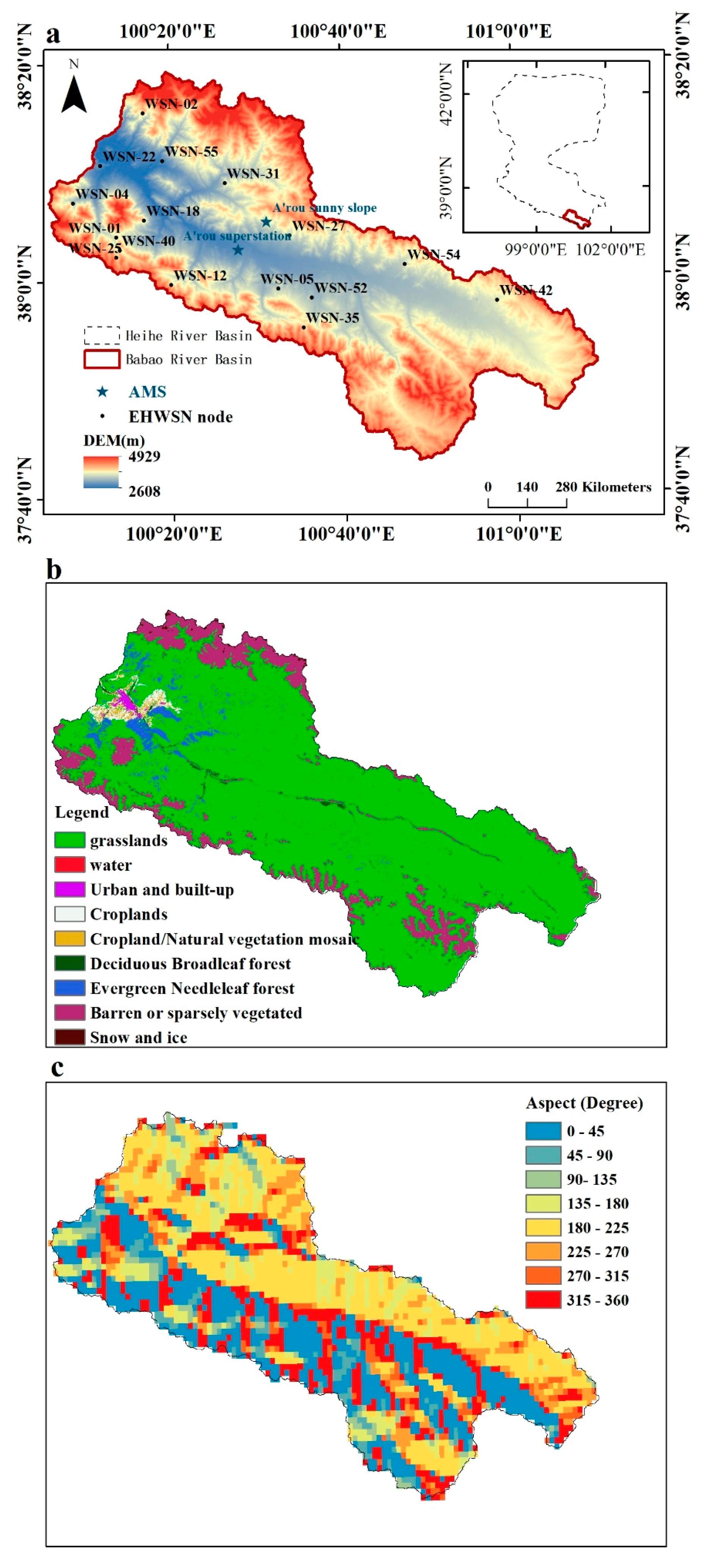
2.1. Study Area
2.2. In Situ Measurements
2.3. Remote Sensing Products
3. Methods
3.1. The Bayesian Linear Regression (BLR) Upscaling Algorithm
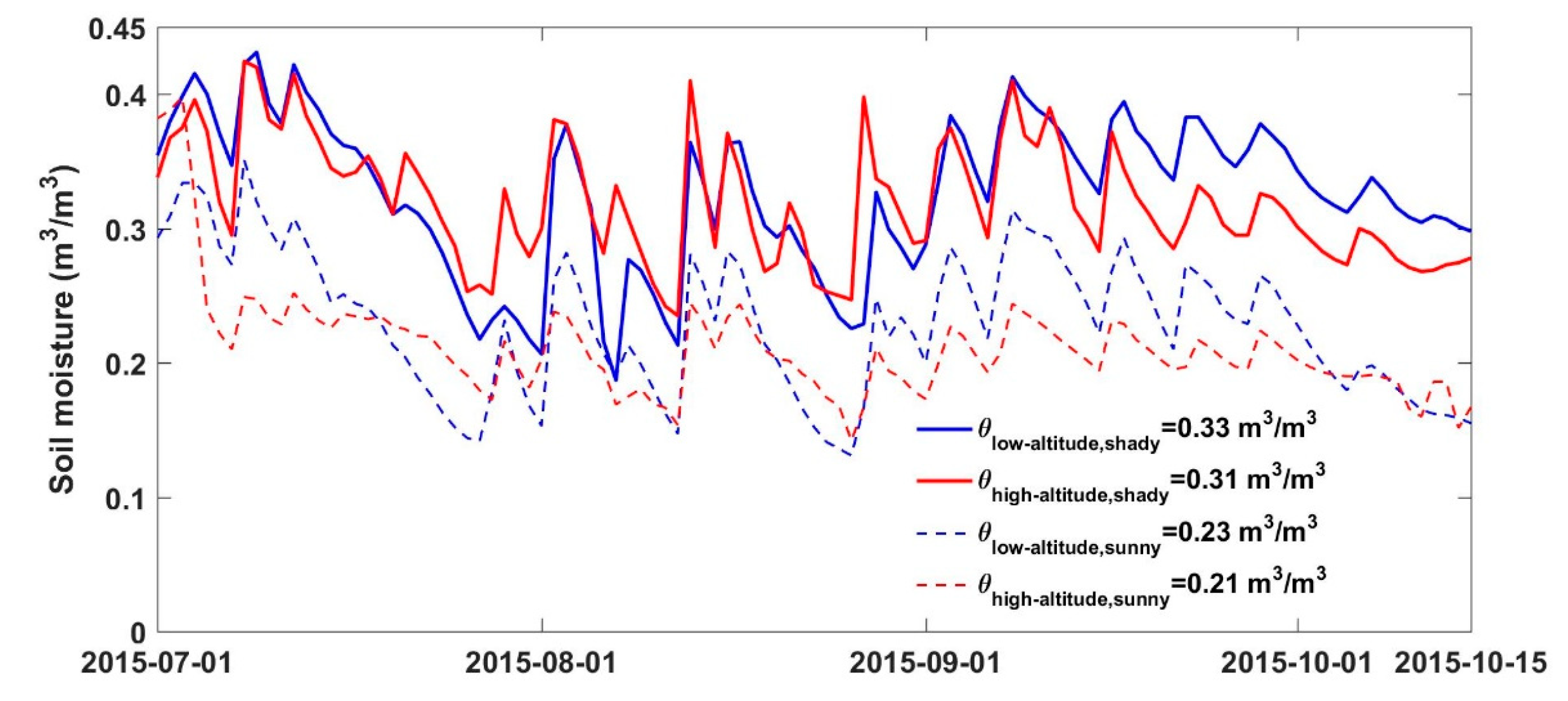
3.2. Representative Soil Moisture
- (a)
- Retrieval of
- (b)
- Retrieval of by combining and .
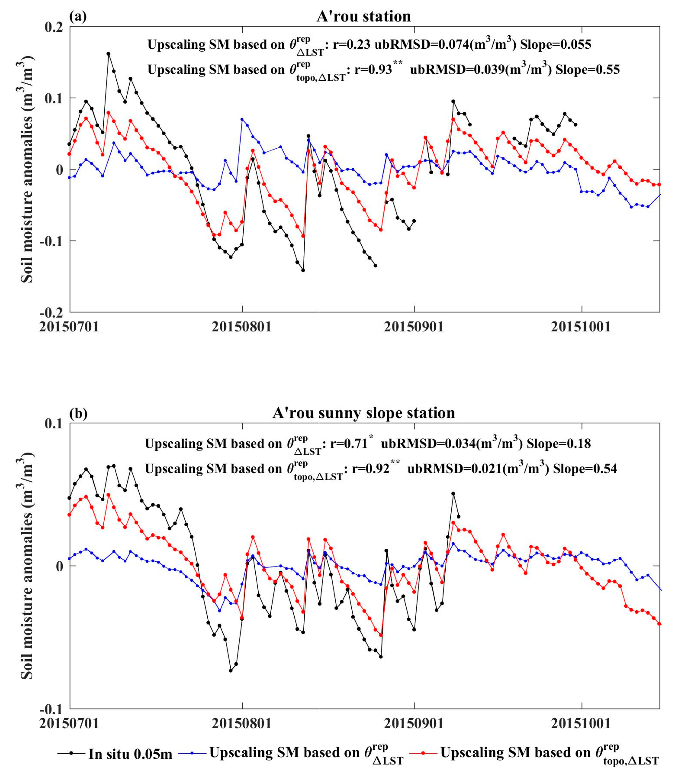
3.3. Validation
3.4. Evaluation Metrics
4. Results
4.1. Representative Soil Moisture
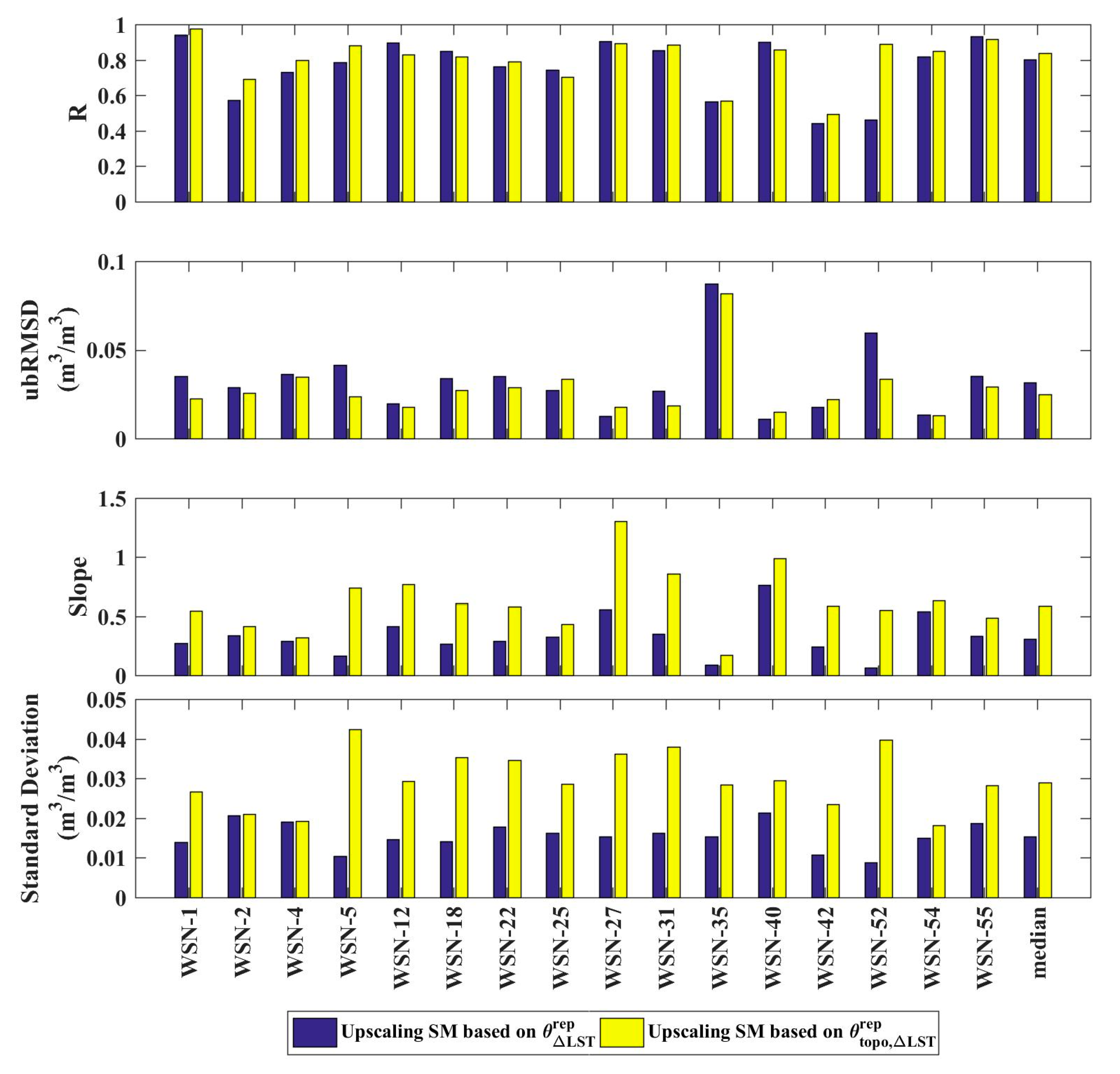
4.2. The BLR Performance Evaluation
5. Discussion
6. Conclusions
Author Contributions
Funding
Acknowledgments
Conflicts of Interest
References
- Wigneron, J.-P.; Jackson, T.; O’neill, P.; De Lannoy, G.; De Rosnay, P.; Walker, J.; Ferrazzoli, P.; Mironov, V.; Bircher, S.; Grant, J. Modelling the passive microwave signature from land surfaces: A review of recent results and application to the L-band SMOS & SMAP soil moisture retrieval algorithms. Remote Sens. Environ. 2017, 192, 238–262. [Google Scholar]
- Fan, L.; Wigneron, J.-P.; Xiao, Q.; Al-Yaari, A.; Wen, J.; Martin-StPaul, N.; Dupuy, J.-L.; Pimont, F.; Al Bitar, A.; Fernandez-Moran, R. Evaluation of microwave remote sensing for monitoring live fuel moisture content in the Mediterranean region. Remote Sens. Environ. 2018, 205, 210–223. [Google Scholar] [CrossRef]
- Al-Yaari, A.; Wigneron, J.-P.; Ducharne, A.; Kerr, Y.; De Rosnay, P.; De Jeu, R.; Govind, A.; Al Bitar, A.; Albergel, C.; Munoz-Sabater, J. Global-scale evaluation of two satellite-based passive microwave soil moisture datasets (SMOS and AMSR-E) with respect to Land Data Assimilation System estimates. Remote Sens. Environ. 2014, 149, 181–195. [Google Scholar] [CrossRef]
- Merlin, O.; Walker, J.P.; Chehbouni, A.; Kerr, Y. Towards deterministic downscaling of SMOS soil moisture using MODIS derived soil evaporative efficiency. Remote Sens. Environ. 2008, 112, 3935–3946. [Google Scholar] [CrossRef]
- Peng, J.; Shen, H.; Wu, J.S. Soil moisture retrieving using hyperspectral data with the application of wavelet analysis. Environ. Earth Sci. 2013, 69, 279–288. [Google Scholar] [CrossRef]
- Kerr, Y.H.; Al-Yaari, A.; Rodriguez-Fernandez, N.; Parrens, M.; Molero, B.; Leroux, D.; Bircher, S.; Mahmoodi, A.; Mialon, A.; Richaume, P. Overview of SMOS performance in terms of global soil moisture monitoring after six years in operation. Remote Sens. Environ. 2016, 180, 40–63. [Google Scholar] [CrossRef]
- Njoku, E.G.; Jackson, T.J.; Lakshmi, V.; Chan, T.K.; Nghiem, S.V. Soil moisture retrieval from AMSR-E. IEEE Trans. Geosci. Remote Sens. 2003, 41, 215–229. [Google Scholar] [CrossRef]
- Entekhabi, D.; Njoku, E.G.; O’Neill, P.E.; Kellogg, K.H.; Crow, W.T.; Edelstein, W.N.; Entin, J.K.; Goodman, S.D.; Jackson, T.J.; Johnson, J. The soil moisture active passive (SMAP) mission. Proc. IEEE 2010, 98, 704–716. [Google Scholar] [CrossRef]
- Das, N.N.; Entekhabi, D.; Njoku, E.G. An algorithm for merging SMAP radiometer and radar data for high-resolution soil-moisture retrieval. IEEE Trans. Geosci. Remote Sens. 2011, 49, 1504–1512. [Google Scholar] [CrossRef]
- Merlin, O.; Rudiger, C.; Al Bitar, A.; Richaume, P.; Walker, J.P.; Kerr, Y.H. Disaggregation of SMOS soil moisture in Southeastern Australia. IEEE Trans. Geosci. Remote Sens. 2012, 50, 1556–1571. [Google Scholar] [CrossRef]
- Piles, M.; Sánchez, N.; Vall-llossera, M.; Camps, A.; Martínez-Fernández, J.; Martínez, J.; González-Gambau, V. A downscaling approach for SMOS land observations: Evaluation of high-resolution soil moisture maps over the Iberian Peninsula. IEEE J. Sel. Top. Appl. Earth Obs. Remote Sens. 2014, 7, 3845–3857. [Google Scholar] [CrossRef]
- Chauhan, N.; Miller, S.; Ardanuy, P. Spaceborne soil moisture estimation at high resolution: A microwave-optical/IR synergistic approach. Int. J. Remote Sens. 2003, 24, 4599–4622. [Google Scholar] [CrossRef]
- Peng, J.; Loew, A.; Merlin, O.; Verhoest, N.E. A review of spatial downscaling of satellite remotely sensed soil moisture. Rev. Geophys. 2017, 55, 341–366. [Google Scholar] [CrossRef]
- Kerr, Y.H.; Waldteufel, P.; Wigneron, J.-P.; Martinuzzi, J.; Font, J.; Berger, M. Soil moisture retrieval from space: The Soil Moisture and Ocean Salinity (SMOS) mission. IEEE Trans. Geosci. Remote Sens. 2001, 39, 1729–1735. [Google Scholar] [CrossRef]
- Qiu, Y.; Fu, B.; Wang, J.; Chen, L. Spatial variability of soil moisture content and its relation to environmental indices in a semi-arid gully catchment of the Loess Plateau, China. J. Arid Environ. 2001, 49, 723–750. [Google Scholar] [CrossRef]
- Bárdossy, A.; Lehmann, W. Spatial distribution of soil moisture in a small catchment. Part 1: Geostatistical analysis. J. Hydrol. 1998, 206, 1–15. [Google Scholar] [CrossRef]
- Anderson, S.P.; Bales, R.C.; Duffy, C.J. Critical Zone Observatories: Building a network to advance interdisciplinary study of Earth surface processes. Mineral. Mag. 2008, 72, 7–10. [Google Scholar] [CrossRef]
- Li, X.; Cheng, G.; Liu, S.; Xiao, Q.; Ma, M.; Jin, R.; Che, T.; Liu, Q.; Wang, W.; Qi, Y. Heihe watershed allied telemetry experimental research (HiWATER): Scientific objectives and experimental design. Bull. Am. Meteorol. Soc. 2013, 94, 1145–1160. [Google Scholar] [CrossRef]
- Greifeneder, F.; Notarnicola, C.; Bertoldi, G.; Niedrist, G.; Wagner, W. From point to pixel scale: An upscaling approach for in situ soil moisture measurements. Vadose Zone J. 2016, 15. [Google Scholar] [CrossRef]
- Kang, J.; Jin, R.; Li, X. Regression kriging-based upscaling of soil moisture measurements from a wireless sensor network and multiresource remote sensing information over heterogeneous cropland. IEEE Geosci. Remote Sens. Lett. 2015, 12, 92–96. [Google Scholar] [CrossRef]
- Gao, S.; Zhu, Z.; Liu, S.; Jin, R.; Yang, G.; Tan, L. Estimating the spatial distribution of soil moisture based on Bayesian maximum entropy method with auxiliary data from remote sensing. Int. J. Appl. Earth Obs. Geoinform. 2014, 32, 54–66. [Google Scholar] [CrossRef]
- Fan, L.; Xiao, Q.; Wen, J.; Liu, Q.; Jin, R.; You, D.; Li, X. Mapping high-resolution soil moisture over heterogeneous cropland using multi-resource remote sensing and ground observations. Remote Sens. 2015, 7, 13273–13297. [Google Scholar] [CrossRef]
- Crow, W.T.; Berg, A.A.; Cosh, M.H.; Loew, A.; Mohanty, B.P.; Panciera, R.; de Rosnay, P.; Ryu, D.; Walker, J.P. Upscaling sparse ground-based soil moisture observations for the validation of coarse-resolution satellite soil moisture products. Rev. Geophys. 2012, 50. [Google Scholar] [CrossRef]
- Fan, L.; Xiao, Q.; Wen, J.; Liu, Q.; Tang, Y.; You, D.; Wang, H.; Gong, Z.; Li, X. Evaluation of the airborne CASI/TASI Ts-VI space method for estimating near-surface soil moisture. Remote Sens. 2015, 7, 3114–3137. [Google Scholar] [CrossRef]
- Kang, J.; Jin, R.; Li, X.; Ma, C.; Qin, J.; Zhang, Y. High spatio-temporal resolution mapping of soil moisture by integrating wireless sensor network observations and MODIS apparent thermal inertia in the Babao River Basin, China. Remote Sens. Environ. 2017, 191, 232–245. [Google Scholar] [CrossRef]
- Djamai, N.; Magagi, R.; Goïta, K.; Merlin, O.; Kerr, Y.; Roy, A. A combination of DISPATCH downscaling algorithm with CLASS land surface scheme for soil moisture estimation at fine scale during cloudy days. Remote Sens. Environ. 2016, 184, 1–14. [Google Scholar] [CrossRef]
- Chen, T.; Martin, E. Bayesian linear regression and variable selection for spectroscopic calibration. Anal. Chim. Acta 2009, 631, 13–21. [Google Scholar] [CrossRef]
- Qin, J.; Yang, K.; Lu, N.; Chen, Y.; Zhao, L.; Han, M. Spatial upscaling of in-situ soil moisture measurements based on MODIS-derived apparent thermal inertia. Remote Sens. Environ. 2013, 138, 1–9. [Google Scholar] [CrossRef]
- Hassan, Q.K.; Bourque, C.P.-A.; Meng, F.-R.; Cox, R.M. A wetness index using terrain-corrected surface temperature and normalized difference vegetation index derived from standard MODIS products: An evaluation of its use in a humid forest-dominated region of eastern Canada. Sensors 2007, 7, 2028–2048. [Google Scholar] [CrossRef]
- Cherubini, F.; Vezhapparambu, S.; Bogren, W.; Astrup, R.; Strømman, A.H. Spatial, seasonal, and topographical patterns of surface albedo in Norwegian forests and cropland. Int. J. Remote Sens. 2017, 38, 4565–4586. [Google Scholar] [CrossRef]
- Li, X.; Li, X.; Li, Z.; Ma, M.; Wang, J.; Xiao, Q.; Liu, Q.; Che, T.; Chen, E.; Yan, G. Watershed allied telemetry experimental research. J. Geophys. Res. Atmos. 2009, 114. [Google Scholar] [CrossRef]
- Yong, G.; Jianghao, W.; Jinfeng, W.; Rui, J.; Maogui, H. Regression Kriging model-based sampling optimization design for the eco-hydrology wireless sensor network. Adv. Earth Sci. 2012, 27, 1006–1013. [Google Scholar]
- Kang, J.; Tan, J.; Jin, R.; Li, X.; Zhang, Y. Reconstruction of MODIS land surface temperature products based on multi-temporal information. Remote Sens. 2018, 10, 1112. [Google Scholar] [CrossRef]
- Jin, R.; Li, X.; Liu, S. Understanding the heterogeneity of soil moisture and evapotranspiration using multiscale observations from satellites, airborne sensors, and a ground-based observation matrix. IEEE Geosci. Remote Sens. Lett. 2017, 14, 2132–2136. [Google Scholar] [CrossRef]
- Liu, S.; Li, X.; Xu, Z.; Che, T.; Xiao, Q.; Ma, M.; Liu, Q.; Jin, R.; Guo, J.; Wang, L. The Heihe Integrated Observatory Network: A Basin-Scale Land Surface Processes Observatory in China. Vadose Zone J. 2018, 17. [Google Scholar] [CrossRef]
- Wan, Z.; Zhang, Y.; Zhang, Q.; Li, Z.-L. Quality assessment and validation of the MODIS global land surface temperature. Int. J. Remote Sens. 2004, 25, 261–274. [Google Scholar] [CrossRef]
- Westermann, S.; Langer, M.; Boike, J. Spatial and temporal variations of summer surface temperatures of high-arctic tundra on Svalbard—implications for MODIS LST based permafrost monitoring. Remote Sens. Environ. 2011, 115, 908–922. [Google Scholar] [CrossRef]
- Tachikawa, T.; Hato, M.; Kaku, M.; Iwasaki, A. Characteristics of ASTER GDEM version 2. In Proceedings of the 2011 IEEE International Geoscience and Remote Sensing Symposium (IGARSS), Vancouver, BC, Canada, 24–29 July 2011; pp. 3657–3660. [Google Scholar]
- Zhong, B.; Yang, A.; Nie, A.; Yao, Y.; Zhang, H.; Wu, S.; Liu, Q. Finer resolution land-cover mapping using multiple classifiers and multisource remotely sensed data in the Heihe River Basin. IEEE J. Sel. Top. Appl. Earth Obs. Remote Sens. 2015, 8, 4973–4992. [Google Scholar] [CrossRef]
- Cawley, G.C.; Talbot, N.L. Efficient leave-one-out cross-validation of kernel fisher discriminant classifiers. Pattern Recognit. 2003, 36, 2585–2592. [Google Scholar] [CrossRef]
- Al-Yaari, A.; Wigneron, J.-P.; Dorigo, W.; Colliander, A.; Pellarin, T.; Hahn, S.; Mialon, A.; Richaume, P.; Fernandez-Moran, R.; Fan, L. Assessment and inter-comparison of recently developed/reprocessed microwave satellite soil moisture products using ISMN ground-based measurements. Remote Sens. Environ. 2019, 224, 289–303. [Google Scholar] [CrossRef]
- Al-Yaari, A.; Wigneron, J.-P.; Kerr, Y.; Rodriguez-Fernandez, N.; O’Neill, P.; Jackson, T.; De Lannoy, G.; Al Bitar, A.; Mialon, A.; Richaume, P. Evaluating soil moisture retrievals from ESA’s SMOS and NASA’s SMAP brightness temperature datasets. Remote Sens. Environ. 2017, 193, 257–273. [Google Scholar] [CrossRef]
- Entekhabi, D.; Reichle, R.H.; Koster, R.D.; Crow, W.T. Performance metrics for soil moisture retrievals and application requirements. J. Hydrometeorol. 2010, 11, 832–840. [Google Scholar] [CrossRef]
- Malbéteau, Y.; Merlin, O.; Gascoin, S.; Gastellu, J.-P.; Mattar, C.; Olivera-Guerra, L.; Khabba, S.; Jarlan, L. Normalizing land surface temperature data for elevation and illumination effects in mountainous areas: A case study using ASTER data over a steep-sided valley in Morocco. Remote Sens. Environ. 2017, 189, 25–39. [Google Scholar] [CrossRef]
- Ermida, S.L.; DaCamara, C.C.; Trigo, I.F.; Pires, A.C.; Ghent, D.; Remedios, J. Modelling directional effects on remotely sensed land surface temperature. Remote Sens. Environ. 2017, 190, 56–69. [Google Scholar] [CrossRef]
- Raz-Yaseef, N.; Rotenberg, E.; Yakir, D. Effects of spatial variations in soil evaporation caused by tree shading on water flux partitioning in a semi-arid pine forest. Agric. For. Meteorol. 2010, 150, 454–462. [Google Scholar] [CrossRef]
- Sandholt, I.; Rasmussen, K.; Andersen, J. A simple interpretation of the surface temperature/vegetation index space for assessment of surface moisture status. Remote Sens. Environ. 2002, 79, 213–224. [Google Scholar] [CrossRef]
- Carlson, T. An overview of the” triangle method” for estimating surface evapotranspiration and soil moisture from satellite imagery. Sensors 2007, 7, 1612–1629. [Google Scholar] [CrossRef]
- Sobrino, J.; Franch, B.; Mattar, C.; Jiménez-Muñoz, J.; Corbari, C. A method to estimate soil moisture from Airborne Hyperspectral Scanner (AHS) and ASTER data: Application to SEN2FLEX and SEN3EXP campaigns. Remote Sens. Environ. 2012, 117, 415–428. [Google Scholar] [CrossRef]
- Ge, Y.; Wang, J.; Heuvelink, G.B.; Jin, R.; Li, X.; Wang, J. Sampling design optimization of a wireless sensor network for monitoring ecohydrological processes in the Babao River basin, China. Int. J. Geogr. Inf. Sci. 2015, 29, 92–110. [Google Scholar] [CrossRef]


| Station | Type | Observation Period during 2015 | Observation Depth | Temporal Resolution |
|---|---|---|---|---|
| WSN-01 | EHWSN | 1 January to 25 August | 4, 10, 20 cm | 5 min |
| WSN-02 | EHWSN | 1 January to 23 October | 4, 10, 20 cm | 5 min |
| WSN-04 | EHWSN | 1 January to 31 December | 4, 10, 20 cm | 5 min |
| WSN-05 | EHWSN | 1 January to 31 December | 4, 10, 20 cm | 5 min |
| WSN-12 | EHWSN | 13 March to 31 December | 4, 10, 20 cm | 5 min |
| WSN-18 | EHWSN | 1 January to 31 December | 4, 10, 20 cm | 5 min |
| WSN-22 | EHWSN | 1 January to 31 December | 4, 10, 20 cm | 5 min |
| WSN-25 | EHWSN | 1 January to 31 December | 4, 10, 20 cm | 5 min |
| WSN-27 | EHWSN | 6 August to 31 December | 4, 10, 20 cm | 5 min |
| WSN-31 | EHWSN | 1 January to 31 December | 4, 10, 20 cm | 5 min |
| WSN-35 | EHWSN | 1 January to 31 December | 4, 10, 20 cm | 5 min |
| WSN-40 | EHWSN | 1 January to 29 October | 4, 10, 20 cm | 5 min |
| WSN-42 | EHWSN | 1 January to 31 December | 4, 10, 20 cm | 5 min |
| WSN-52 | EHWSN | 30 January to 31 December | 4, 10, 20 cm | 5 min |
| WSN-54 | EHWSN | 1 January to 31 December | 4, 10, 20 cm | 5 min |
| WSN-55 | EHWSN | 1 January to 31 December | 4, 10, 20 cm | 5 min |
| A’rou superstation | AMS | 1 January to 31 December | 2, 4, 6, 10, 15, 20, 30, 40, 60, 80, 120, 160, 200, 240, 280, 320 cm | 10 min |
| A’rou sunny slope | AMS | 1 January to 9 September | 4, 10, 20, 40, 80, 120, 160 cm | 10 min |
© 2019 by the authors. Licensee MDPI, Basel, Switzerland. This article is an open access article distributed under the terms and conditions of the Creative Commons Attribution (CC BY) license (http://creativecommons.org/licenses/by/4.0/).
Share and Cite
Fan, L.; Al-Yaari, A.; Frappart, F.; Swenson, J.J.; Xiao, Q.; Wen, J.; Jin, R.; Kang, J.; Li, X.; Fernandez-Moran, R.; et al. Mapping Soil Moisture at a High Resolution over Mountainous Regions by Integrating In Situ Measurements, Topography Data, and MODIS Land Surface Temperatures. Remote Sens. 2019, 11, 656. https://doi.org/10.3390/rs11060656
Fan L, Al-Yaari A, Frappart F, Swenson JJ, Xiao Q, Wen J, Jin R, Kang J, Li X, Fernandez-Moran R, et al. Mapping Soil Moisture at a High Resolution over Mountainous Regions by Integrating In Situ Measurements, Topography Data, and MODIS Land Surface Temperatures. Remote Sensing. 2019; 11(6):656. https://doi.org/10.3390/rs11060656
Chicago/Turabian StyleFan, Lei, A. Al-Yaari, Frédéric Frappart, Jennifer J. Swenson, Qing Xiao, Jianguang Wen, Rui Jin, Jian Kang, Xiaojun Li, R. Fernandez-Moran, and et al. 2019. "Mapping Soil Moisture at a High Resolution over Mountainous Regions by Integrating In Situ Measurements, Topography Data, and MODIS Land Surface Temperatures" Remote Sensing 11, no. 6: 656. https://doi.org/10.3390/rs11060656
APA StyleFan, L., Al-Yaari, A., Frappart, F., Swenson, J. J., Xiao, Q., Wen, J., Jin, R., Kang, J., Li, X., Fernandez-Moran, R., & Wigneron, J.-P. (2019). Mapping Soil Moisture at a High Resolution over Mountainous Regions by Integrating In Situ Measurements, Topography Data, and MODIS Land Surface Temperatures. Remote Sensing, 11(6), 656. https://doi.org/10.3390/rs11060656