Did Ecological Restoration Hit Its Mark? Monitoring and Assessing Ecological Changes in the Grain for Green Program Region Using Multi-source Satellite Images

Abstract

Ecological restoration programs are expected to control environmental deterioration and enhance ecosystem functions under a scenario of increasing human disturbance. The largest ecological restoration program ever implemented in China, the first round of the countrywide Grain for Green Program (GGP), finished in 2010. However, it is not known whether the ecological changes that resulted from the GGP met the restoration goal across the whole implementation region. In this study, we monitored and assessed the ecological changes in the whole GGP region in China over the lifetime of the first round of implementation (2000–2010), by establishing a comprehensive assessment indicator system composed of ecosystem pattern, ecosystem quality (EQ), and key ecosystem services (ESs). Remote sensing interpretation, ecological model simulations based on multi-source images, and trend analysis were used to generate land use and land cover (LULC) datasets and estimate ES and ESs indicators. Results showed that while forest increased by 0.77%, artificial land increased more intensely by 22.38%, and cropland and grassland decreased by 1.81% and 0.68%, respectively. The interconversion of cropland and forest played a primary role in ecosystem pattern change. The increase in ecosystem quality measures, including fractional vegetation cover (0.1459% yr⁻¹), leaf area index (0.0121 yr⁻¹), and net primary productivity (2.6958 gC m⁻² yr⁻¹), and the mitigation of ecosystem services deterioration in soil water loss (−0.0841 t ha yr⁻¹) and soil wind loss (−1.0071 t ha yr⁻¹) in the GGP region, indicated the positive ecological change in the GGP region to some extent, while southern GGP subregions improved more than the those in the north on the whole. The GGP implementation other than climate change impacted ecological change, with contributions of 14.23%, 9.94%, 8.23%, 30.45%, and 18.05% in the ecological outputs mentioned above, respectively. However, the water regulation did not improve (−2283 t km⁻² yr⁻¹), revealing trade-offs between ecosystem services and inappropriate afforestation in ecological restoration programs. Future GGP implementation should change the practice of large-scale afforestation, and focus more on the restoration of existing forest and cultivation of young plantings, formulating rational and specific plans and designs for afforestation areas through the establishment of near-natural vegetation communities, instead of single-species plantations, guided by regional climate and geographical characteristics.

1. Introduction

Humans have displayed a history of deforesting and changing land use and land cover since farming began. China’s environmental problems are among the most severe of any major country, because of the need for food security for its large population and the pursuit of high economic growth [1]. From the 1950s to the 1980s, China experienced severe losses of forest and grassland because of large-scale deforestation and grassland reclamation for crop production and industrial construction [2,3,4,5]. This pattern of changing land use has led to severe soil erosion [6]; land desertification [7,8]; loss of biodiversity [9,10]; drying rivers and shrinking lakes [11]; and the frequent occurrence of dust storms, floods, and drought [1,12,13].

To address these problems and maintain environmental sustainability, several countrywide ecological restoration programs have been implemented [2,14]. The Grain for Green Program (GGP), also known as the Sloping Land Conversion Program (SLCP), is regarded as the largest ecological restoration program ever implemented in a developing country [4,15]. The GGP, originally planned for 2001–2010 (the first round), aimed to set aside 14.67 million ha of cropland (4.4 million ha with slopes greater than 25°) and afforest a roughly equal area of wasteland by 2010 [16]. By the end of 2015, the Chinese government had achieved its ambition to increase forest by approximately 29.87 million ha, with a total investment of approximately 405.66 billion RMB (US$58.52 billion) [17]. A new round was launched at the end of 2014 [18], and the implementation region was expanded at the end of 2015 [19]. An assessment of the impact of the first round of GGP on ecosystems could provide insights into future ecological restoration, and provide input into ecological programs initiated by other countries’ governments all around the world.

Previous studies have evaluated the ecological changes brought about by the GGP restoration program from different perspectives, including land use and land cover (LULC) change, vegetation condition, net primary productivity (NPP), and ecosystem services, since the program was designed to convert farmland to forest and grassland, and further reduce soil erosion and desertification [20,21,22,23]. Zhu & Wang [24] detected land cover change in Ansai County and found that farmland had been reduced overall from 18.12% to 13.58% in 2004–2010, while forest increased from 14.60% to 37.95%. Li et al. [25] investigated the vegetation in Bijie Prefecture and found that it had been significantly improved, but the trend of degradation had not been reversed in the east of the region. Feng et al. [26] reported that the NPP and evapotranspiration (ET) in Loess Plateau had increased by 9.3 gCm⁻² and 4.3 mm per year, respectively, in 2000–2010, but lost soil moisture of 2.4 mm yr⁻¹ and runoff of 0.5 mm yr⁻¹ simultaneously. Wang et al. [19] stated that the transformation from non-irrigated farmland to forestland could potentially improve soil conservation by 24.89%, but the increase extent of GGP implementation decreased NPP and water yield at the sub-watershed scale. With the analysis of different ecological variables, these findings underscore the complexity and trade-offs behind the anthropogenic program implementation. Although previous studies have investigated eco-environmental change in the GGP region, most have focused on the local or regional scale, rather than the national scale. Moreover, the impact of climate change on ecosystems has often been neglected, which may cause unforeseen errors in the assessment.

In this paper, we monitor and assess the ecological changes in the whole region where the GGP was implemented in China from 2000 to 2010 using remote sensing and modelling techniques along with trend analysis, based on a comprehensive assessment indicator system established to reflect changes in ecosystem pattern, ecosystem quality, and key ecosystem services. Our study attempts to answer the following questions: (1) did the first round of the GGP achieve its goal of enhancing local ecological and environmental conditions after investing huge amounts of capital and resources?; (2) how can these ecological changes be measured comprehensively and effectively?; (3) did the whole GGP implementation region show a notable positive trend of ecological change?; and (4) to what extent did the GGP implementation improve the ecological environment after excluding the influence of climate change?

2. Materials and Methods

2.1. Subregions

The GGP started with a pilot program in three provinces in 1999 and was formally launched in 2002. It expanded to a total of 1897 county units across 25 provinces (autonomous regions and municipalities) and the Xinjiang Production and Construction Corps—a wide area with huge ecological and economic heterogeneity, covering 76.77% of China—and involved tens of millions of rural households [16]. Following the principle of hazard prevention, the GGP implementation area was divided into 10 subregions by China’s State Forestry Administration (SFA) according to the risk of soil erosion, wind erosion, and desertification; local hydrothermal conditions; and landform characteristics: the Alpines-Gorges Region in Southwestern China (AGRSC), the Mountains-Hills Region in Sichuan, Chongqing, Hubei and Hunan Province (MHRSCHH), the Low Mountains-Hills Region in Middle and Lower Yangtze Plain (LMHRMLYP), the Yunnan-Guizhou Plateau Region (YGPR), the Mountains-Hills Region in Hainan and Guangxi Province (MHRHG), the Alpine Steppe and Meadow Region in the source of Yangtze River and Yellow River (ASMRYY), the Arid Desert Region in Xinjiang Province (ADRX), the Hills-Gullies Region in Loess Plateau (HGRLP), the Arid and Semi-arid Region in Northern China (ASRNC), and the Mountains-Sands Region in Northeastern China (MSRNC) (Figure 1). By taking different conservation measures in each subregion (Table 1), the government hoped to recover and enhance natural ecosystems more efficiently [27].

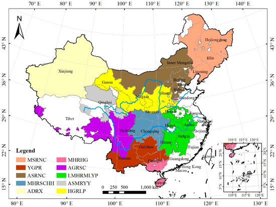
Figure 1. Distribution of subregions involved in the Grain for Green Program (GGP). For the full names and description of each region, see Table 1.

Table 1. Natural characteristics and restoration measures in the Grain for Green Program (GGP) subregions.

Classification	Subregions	Natural Characteristics	Restoration Measures
Northern subregions	Mountains-Sands Region in Northeastern China (MSRNC)	Transits from continental monsoon zone in the east to temperate continental semi-arid zone in the west. Mountains, hills and plains are interspaced. Land use is a mix of agriculture, pasture and forest. Grassland degradation is severe in the west.	Strive to develop artificial forest mainly composed of shelterbelts and timber tree on the basis of protection of natural forests. Afforestation for firewood and national defense as appropriate. Develop economic forest and medical herbs by 0.1 ha per capita on gently sloping land where the erosion risk is low. Emphasize the replanting of ecological forests, taking account also of economic, forage and firewood forests and high-quality pasture.
	Arid and Semi-arid Region in Northern China (ASRNC)	Transits from continental monsoon zone in the east to temperate continental semi-arid zone in the west, with annual average precipitation ranging from 550 mm to 150 mm from southeast to northwest. Relatively flat terrain consists of plateau and plain. Agriculture, pasture and forest are interspaced in the east, whereas grassland and sparse vegetation occupies the west, with serious desertification.	Carry out artificial forestation and grassland planting, mainly by shrub-grass, on returned farmland. Develop high-standard farmland, economic forest and medical herbs by 0.1 ha per capita on gently sloping land where the erosion risk is low. Return farmland by 0.1 ha per capita on sloping and hummock land. Emphasize replanting of ecological forest, taking account also of forage and firewood forests. The proportion of forest and grassland for forage, forest for firewood must be kept under 30% and 10%, respectively.
	Arid Desert Region in Xinjiang province (ADRX)	Extremely arid with annual precipitation mostly below 200 mm, sparse vegetation, frequent sandstorms, desert and Gobi. Water shortages and desert expansion make the ecological conditions worse.	Return and revegetate all frontier farmland suffering severe desertification. Establish windbreak and sand-fixation forest systems with proper combination of trees, shrubs and herbs. Control sand movement and fix dunes by fencing, laying barriers and planting shrubbery belt on the windward slope of dunes within 100 m of their upwind direction. Develop high-standard farmland or pasture by 0.1 ha per capita, and economic forest by 0.07 ha per capita on the land where the desertification risk is low. Emphasis on replanting wind-breaks and sand-fixing forest and developing a few forage, firewood, timber and economic forests.
	Alpine Steppe and Meadow Region in the source of Yangtze River and Yellow River (ASMRYY)	High altitude, cold, dry with little rain, belongs to temperate continental semi-arid climate with annual precipitation ranging from 500 mm to 700 mm. Large temperature difference between day and night, strong wind and plenty of sand, low and sparse vegetation, mostly grassland. Grassland degradation and desertification is severe, soil erosion is being aggravated.	Restore all sloping cropland above 25° to forest or grassland by artificial afforestation and grass planting. Restore grazing land, barren hills and wasteland by closing off hillsides for forest and grass conservation or artificial afforestation. Emphasis on replanting ecological forest and grass, and developing a few forage forests, grass and firewood forests.
	Hills-Gullies Region in Loess Plateau (HGRLP)	Semi-arid continental monsoon climate with annual precipitation ranging from 350 mm to 600 mm. The terrain consists of tablelands, hummocks mounds, ditches and rivers. The broken topography, ravines and gullies, loose soil and water flow from the Yellow River, yield the most serious soil-water erosion in China.	Return all sloping cropland above 25° that is prone to soil erosion to soil and water conservation forest, and develop some forage forest for animal husbandry. Develop basic farmland by 0.1 ha per capita on gently sloping land where the erosion risk is low, and increase economic forest by 0.07 ha per capita through ridge, slope and soil preparation. Emphasis on replanting ecological forest and appropriate development of forage forest and economic forest (7:2:1).
Southern subregions	Alpines-Gorges Region in Southwestern China (AGRSC)	Plateau alpine climate, annual precipitation ranges from 500 mm to 1500 mm. High terrain, steep slopes, mainly montane cinnamon soil, poor soil on sunny slopes with water deficits, naturally poor regeneration of forest.	Return all sloping cropland above 25° with shallow soil to forest; reforest sloping land with gentler gradient and thicker soil after partial transformation into high-standard farmland by 0.1 ha per capita. Emphasis on planting of ecological forest and appropriate development of timber and firewood forest and high-quality pasture.
	Mountains-Hills Region in Sichuan, Chongqing, Hubei and Hunan province (MHRSCHH)	Subtropical humid monsoon climate, annual precipitation ranges from 700 mm to 1200 mm, diverse landforms with great elevation difference, complex topography, and rich natural resources.	After guaranteeing high-standard farmland of 0.07 ha per capita, replant all sloping cropland to ecological forest after partial transformation into economic forest by 0.07 ha per capita. Ecological forest and timber forest should account for over 80%, and economic forest for under 20%.
	Low Mountains-Hills Region in Middle and Lower Yangtze Plain (LMHRMLYP)	Subtropical humid monsoon climate, annual precipitation ranges from 1400 mm to 1800 mm, mainly composed of low mountains and hills with a medium elevation ranging from 300 m to 1000 m. Large elevation differences.	Reforest all sloping cropland above 25°, and sloping cropland between 15°–25° with important ecological status. Emphasis on planting ecological forest and grassland, while taking timber and economic forest into consideration. Mainly plant trees, with some shrubs and herbs.
	Yunnan-Guizhou Plateau Region (YGPR)	Characterized by karst landscape, this mountainous plateau is in the central mid-subtropical zone. Annual precipitation is about 1200 mm concentrated in July and August mainly from rainstorms, which result in severe soil loss, debris flows and landslides.	Replant all sloping land above 25° with shallow soil into ecological forest. Sloping cropland between 16° and 25° can develop agroforestry by inter-cultivation of forest and medicinal plants, and the ratio of ecological forest and commercial forest is 3:2. Sloping cropland below 16° with better site condition can develop timber and economic forest under strict controls, after guaranteeing high-standard farmland of 0.07 ha per capita.
	Mountains-Hills Region in Hainan and Guangxi Province (MHRHG)	Tropical and subtropical humid monsoon climate, annual precipitation ranges from 1500 mm to 3000 mm, composed of low mountains and hills with a relative low elevation difference, and rich natural resources.	After guaranteeing high-standard farmland of 0.07 ha per capita, replant all sloping cropland into ecological forest after partial transformation into economic forest of 0.07 ha per capita. Focus on restoring forest for soil and water conservation and developing fast-growing and productive timber and economic forest as appropriate. Ecological forest and timber forest should account for over 80%, and economic forest for under 20%

2.2. Comprehensive Assessment Indicator System for Assessing Ecological Changes from the GGP

To comprehensively and efficiently monitor and assess the ecological changes in the GGP region, we developed an assessment indicator system from three perspectives: ecosystem pattern, ecosystem quality, and key ecosystem services (Table 2). Ecosystem area and ecosystem conversion area, which have been used in many studies, were selected as indicators to reflect changes in the ecosystem pattern [13,20]. As the amount and distribution of vegetation are of prime importance for terrestrial ecosystems [28], the fractional vegetation cover (FVC), leaf area index (LAI), and NPP were chosen to detect ecosystem quality. The FVC is the percentage of vegetation occupying the ground area in a vertical projection [29], while LAI is the ratio of leaf surface area to unit ground surface area [30]. The FVC and LAI parameterize the horizontal and vertical density of vegetation, respectively [31]. They are two important variables used to describe the condition of land surface vegetation, characterize ecosystem changes, and reflect the related biological and physical processes [31,32,33,34]. NPP marks the first visible step of carbon accumulation [35], is a key regulator of ecological processes [36], and is an important component of net ecosystem exchange or net ecosystem productivity. It indicates the metabolism of the ecosystem [37]. Because the FVC, LAI, and NPP vary within a year, we chose the annual maximum value of FVC (FVC_max) and LAI (LAI_max) to reflect the instantaneous vegetation growth status, and the annual average value of NPP (NPP_avg) to reflect the accumulated process of carbon accumulation. In addition, owing to the aims of the GGP were to control soil erosion, mitigate flooding, and prevent sandstorms, we selected three key ecosystem services, water regulation (WR), soil conservation (SC), and sandstorm prevention (SP), to evaluate the enhancement of ecosystem services arising from the program implementation. The annual quantity per unit area of water regulation (WR_pua), soil water loss (SWAL_pua), and soil wind loss (SWIL_pua) were selected as assessment indicators to exclude the influence of area.

Table 2. The comprehensive assessment indicator system for ecological changes of the Grain for Green Program (GGP).

Assessment Categories	Assessment Content	Assessment Indicators	Notes
Ecosystem pattern	Ecosystem composition and distribution	Ecosystem area
	Ecosystem transformation characteristics	Ecosystem transformation area
Ecosystem quality (EQ)	Fractional vegetation cover (FVC)	Annual maximum value of FVC (FVCmax)
	Leaf area index (LAI)	Annual maximum value of LAI (LAImax)	Dimensionless variable
	Net primary productivity (NPP)	Annual average value of NPP (NPPavg)
Key ecosystem services (ES)	Water regulation (WR)	Annual quantity of water regulation per unit area (WRpua)
	Soil conservation (SC)	Annual quantity of soil water loss per unit area (SWALpua)	Contrary indicator, lower values are better
	Sandstorm prevention (SP)	Annual quantity of soil wind loss per unit area (SWILpua)	Contrary indicator, lower values are better

2.3. Generation of Land Use and Land Cover Datasets

Landsat TM/ETM images in 2000 and 2005, and HJ-1 A/B images in 2010 with a 30 m spatial resolution were used to interpret LULC change. Using the FAO Land Cover Classification System (FAO LCCS) tools [38], we classified the images into 38 LULC level II classes [39], and then categorized them into six LULC level I classes, which were forest, grassland, wetland, cropland, artificial land, and other types land, based on the IPCC classification system [40].

We derived the 2010 LULC vector dataset from 2010 HJ-1 A/B images by applying object-oriented automatic classification methods after data preprocessing on a supercomputing platform, with associated data from ground surveys and radar [41]. The overall producer’s accuracy for the 2010 LULC dataset was validated with a total of 31,675 independent ground survey samples based on random sampling and reached 94% and 86% accuracy on average for LULC classes at level I and level II, respectively.

The 2000 and 2005 LULC vector datasets were generated using object-oriented spectrum eigenvectors similarity change detection. The spectrum eigenvectors of a Landsat TM image patch can be regarded as a vector in a six-dimensional feature space, and the smaller the included angle and closer the norm of two vectors, the more similar two patches are. Based on this principle, we used the cosine of the angle between two vectors and the ratio of the vector norm to measure vector similarity, see Song & Yan [42] for details. In eCognition Developer 8.64, we used the 2010 LULC vector dataset generated above to overlap and segment the 2000 and 2005 Landsat TM images with 2010 HJ-1 images at multiple scales, which ensured that the unchanged areas had the same border and provided a priori information on ground objects, enhancing the classification accuracy. We extracted spectrum eigenvectors from each image patch segmented above and calculated the similarity between the images of target years (2000 and 2005) and the base year (2010) to detect LULC change, and then updated the LULC dataset accordingly [43]. A detailed workflow for the LULC datasets in the target years is displayed in Figure 2.

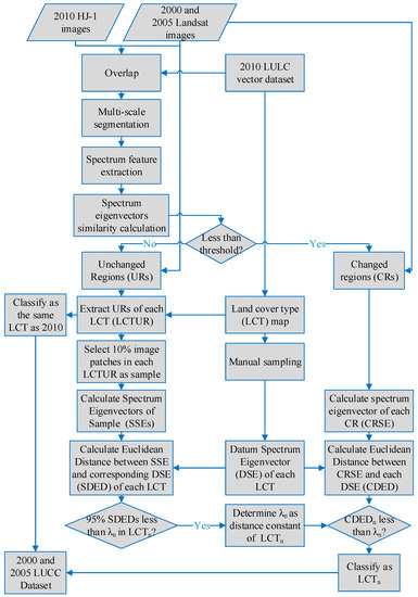
Figure 2. The workflow used to generate the 2000 and 2005 land use and land cover datasets.

2.4. Detection of Ecosystem Pattern Changes

Ecosystem types were consistent with the six LULC level I classes in this study, because we had considered the spectrum characteristics, vegetation coverage, and ecosystem plant community component characteristics in our LULC classification system [44]. Thus, ecosystem pattern changes can be identified through LULC change detection. Here, we employed an LULC transfer matrix to detect the change between LULC types in 2000–2005, 2005–2010, and 2000–2010. The LULC transfer matrix delivers dynamic information on mutual transfer processes between different LULC types from the beginning to the end of a given period; thus it not only includes the static area data of different LULC types at a point in time, but also contains information about the area transferred out and in during a period [45]. The general form of the LULC transfer matrix is:

$${\mathrm{s}}_{\mathrm{ij}}=\left[\begin{array}{cccc}{\mathrm{s}}_{11}& {\mathrm{s}}_{12}& \cdots & {\mathrm{s}}_{1\mathrm{n}}\\ {\mathrm{s}}_{21}& {\mathrm{s}}_{22}& \cdots & {\mathrm{s}}_{2\mathrm{n}}\\ \cdots & \cdots & \cdots & \cdots \\ {\mathrm{s}}_{\mathrm{n}1}& {\mathrm{s}}_{\mathrm{n}2}& \cdots & {\mathrm{s}}_{\mathrm{nn}}\end{array}\right]$$

(1)

where i and j (i, j = 1, 2, …, n) are the LULC type before and after the transformation happened, respectively; n is the total number of LULC types; and s_ij is the area of LULC type i converted to type j over the period, or the area of untransformed LUCC type i when i = j. Each row and column of the transfer matrix, respectively, denotes the source and destination of LULC change.

We rasterized the LULC vector datasets for 2000, 2005, and 2010 into 30 m spatial resolution grids. We calculated the LULC transfer matrix pixel by pixel between each two phases of LULC maps using spatial analyst tools in ArcGIS 10.3.

2.5. Ecosystem Quality Estimation

The FVC was estimated using the pixel dichotomy model [31], which assumes that image pixels are composed of two parts: vegetation-covered and non-vegetation-covered areas [46], and thus the FVC can be defined as follows:

$$\mathrm{FVC}=\frac{\mathrm{NDVI}-\mathrm{NDV}{\mathrm{I}}_{\mathrm{soil}}}{\mathrm{NDV}{\mathrm{I}}_{\mathrm{veg}}-\mathrm{NDV}{\mathrm{I}}_{\mathrm{soil}}}$$

(2)

where NDVI_veg and NDVI_soil are the Normalized Difference Vegetation Index (NDVI) value for pure vegetation pixels and pure bare soil pixels, respectively. We used MOD13A3 data, monthly MODIS NDVI at a 1 km spatial resolution as a gridded level-3 product, as the calculation input after aggregation through the Maximum Value Composite (MVP) approach [47] to obtain the annual maximum value and after time domain processing using a Savitzky-Golay filter [48] to minimize the influence of existing noise.

The LAI was derived from the MODIS MOD15A2 product, which is composited every eight days at a 1 km resolution. We improved our LAI data quality using the temporal spatial filter (TSF) [49] to fill in the spatial and temporal discontinuity of original datasets. We then used MVP to obtain the annual maximum value of LAI.

NPP was evaluated by applying the GLOPEM-CEVSA model [50], which couples a satellite-based model and a process-based model. The model has been validated by carbon flux observations within forest, grassland, and cropland. In the model, NPP is the difference of gross primary productivity (GPP) and autotrophic respiration (R_a), where GPP is estimated by the GLoPEM model, and R_a is divided into maintenance respiration (R_m) and growth respiration (R_g) from four plant parts—thick root, thin root, stem, and leaf—with reference to the process-based BEPS model and Biome-BGC model:

GPP = PAR × FPAR × ε_g

(3)

$${\mathrm{R}}_{\mathrm{a}}={\displaystyle \sum _{\mathrm{i}=1}^4{\mathrm{R}}_{\mathrm{m},\mathrm{i}}+{\mathrm{R}}_{\mathrm{g}}}$$

(4)

R_m,i = M_ir_m,iQ₁₀^(T−Tb)/10

(5)

R_g = r_gGPP

(6)

where PAR (photosynthetically active radiation) was estimated using climatology radiation calculation methods [51] and FPAR (fraction of photosynthetically active radiation) was adapted from satellite remote sensing inversion data based on the canopy radiative transfer model [52]. ε_g, the vegetation light utilization efficiency in the GPP concept, was the product of the maximum possible light utilization efficiency and environment stresses including vapor pressure deficit (VPD), PAR, air temperature, atmospheric CO₂, and soil moisture [53]. M_i and r_m,i are the biomass and maintenance respiration coefficients of the four plant organs, respectively. Q₁₀ represents the change in the maintenance respiration rate when the temperature changes by 10 degrees; T and T_b are the actual temperature and base temperature, respectively; and r_g is the proportional coefficient of total growth respiration to total plant growth. The input meteorological data, including temperature, precipitation, evaporation, and total radiation, were provided by China’s State Meteorological Administration. They were interpolated into grids using thin plate smoothing splines (ANUSPLIN) [54,55].

2.6. Estimation of Ecosystem Services

WR refers to the magnitude of runoff, flood, and aquifer recharge influenced by changes in ecosystems [56,57]. We estimated WR using the Rainfall Storage Method (RSM), which considers the hydrological regulation effect of ecosystems, including forest, grassland, and cropland, compared with bare land [58,59]. RSM can be expressed as follows:

WR = A × (J₀ × K) × (R₀ − R_g)

(7)

where A is the area of the ecosystem; J₀ is the annual average rainfall; K is the ratio of rainfall yielding runoff to total rainfall, which is determined by precipitation and raininess; and R₀ and R_g are the runoff yield rates of bare land and the ecosystem. respectively. The thresholds of rainfall to yield runoff at different locations were collected from published literature, and the single rainfall values at the same locations were derived from three-hour TRMM precipitation data (3B42), which were revised by the measured daily precipitation data of neighboring national meteorological stations. By accumulating single rainfall values greater than the corresponding threshold, we obtained the K values at these single points. With R² = 0.79, a good linear relationship existed between these K values and annual average runoff coefficient at the same locations, thus a national spatial distribution of K value was derived from the national annual average runoff coefficient [60]. The R_g of forest was collected from relevant articles using meta-analysis according to factors such as vegetation types, geographic location, climate zone, and measured surface runoff. The R_g of grassland was calculated according to grassland coverage [61], except for alpine meadows, which adopted the study result of Li et al. [62]. The water conservation amount of floodplain wetlands and inland marshes was calculated at 8100 m³ per hectare according to Meng et al. [63].

SC is the reduction of soil and water loss (SWAL)—the soil erosion resulting from raindrop splash and runoff [64]—by ecosystems through their structures and processes [65,66]. It is the difference between potential and actual soil erosion [19,57]. Therefore, a decline in SWAL implies the improvement of SC. Using the Revised Universal Soil Loss Equation (RUSLE) [64], SWAL can be expressed as:

SWAL = R × K × LS × C × P

(8)

where R is the rainfall-runoff erosivity factor, K is the soil-erodibility factor, LS is the topographic factor, C is the cover-management factor, and P is the support practice factor. In this study, R was calculated using the Daily Rainfall Erosivity Model [67] based on the daily precipitation from national meteorological stations, K was obtained using the soil-erodibility nomograph [68] with the soil dataset from the Second National Soil Survey of China, C was derived according to its relationship with NDVI [69], P was obtained by reference to the USDA Handbook Number 703 and Cai et al. [69], and the LS was computed using the V4.1 SRTM (Shuttle Radar Topography Mission) DEM product at a 90-m spatial resolution by the integrated method of Sun et al. [70].

SP is one of the most important services supplied by ecosystems in arid and semi-arid regions, where vegetation measures help to control desertification and prevent dune movement by fixing dunes and slowing wind velocities [71,72]. The Revised Wind Erosion Equation (RWEQ) is a combination of empirical and process-based models and has been extensively tested in simulating soil loss eroded by wind (SWIL) under broad field conditions [57,73]. As SP is the difference between potential and actual SWIL, the less SWIL, the more SP. SWIL can be expressed as:

Q_max = 109.8(WF × EF × SCF × K′ × COG)

(9)

S = 150.71(WF × EF × SCF × K′ × COG)^−0.3711

(10)

$$\mathrm{SWIL}={\mathrm{Q}}_{\max }[1-{\mathrm{e}}^{{(\frac{\mathrm{x}}{\mathrm{s}})}^2}]$$

(11)

where Q_max is the actual maximum transport capacity, s is the actual critical field length, WF is the weather factor, EF is the soil erodible fraction, SCF is the soil crust factor, K′ is the soil surface roughness, and COG is the combined residue factor. For data sources and processing details, see Gong et al. [74].

2.7. Trend Analysis

The annual trends for ecological changes from 2000 to 2010 were calculated pixel by pixel using the slope equation fitted with ordinary least-squares regression in ENVI 5.4. The slope indicated strong or weak and positive or negative change for the variables [70], with boundaries defined from a 95% confidence interval, which is expressed as follows:

$${\mathrm{slope}}_{\mathrm{i},\mathrm{j}}=\frac{\mathrm{n}\times {\displaystyle {\sum }_{\mathrm{i}=1}^{\mathrm{n}}\mathrm{i}\times {\mathrm{var}}_{\mathrm{i},\mathrm{j}}-{\displaystyle {\sum }_{\mathrm{i}=1}^{\mathrm{n}}\mathrm{i}{\displaystyle {\sum }_{\mathrm{i}=1}^{\mathrm{n}}{\mathrm{var}}_{\mathrm{i},\mathrm{j}}}}}}{\mathrm{n}\times {\displaystyle {\sum }_{\mathrm{i}=1}^{\mathrm{n}}{\mathrm{i}}^2-{\left[{\displaystyle {\sum }_{\mathrm{i}=1}^{\mathrm{n}}\mathrm{i}}\right]}^2}}$$

(12)

where i is the number of years, j is the number of raster pixels, n is the length of study years, and var_i,j stands for the value of the variable (including EQ, ES, and climate indicators) at pixel j in year i.

3. Results

3.1. Changes in Ecosystem Pattern

During the first round of GGP from 2000 to 2010, the ecosystem composition and distribution in the GGP area (Table 3) indicated that the forest ecosystem was the largest ecosystem in the whole GGP area throughout the study period, occupying above 30%, followed by grassland, other types of land, cropland wetland, and artificial land. From 2000 to 2010, forest, wetland, and artificial land showed an increasing trend, while grassland, cropland, and other types of land declined. The artificial land increased dramatically by 22.38%; forest and wetland increased slightly by 0.77% and 1.03%, respectively; and cropland, grassland, and cropland decreased by 1.81%, 0.68%, and 0.41%, respectively. Forest, cropland, and other types of land changed more acutely in the first five years (2000–2005), while grassland, wetland, and artificial land changed more dramatically in the last five years (2005–2010). Forest in the GGP area was mainly distributed in the southern and northeastern subregions, while grassland was largely distributed over the northern subregions. Cropland was concentrated in the eastern plains and the Sichuan Basin (southwestern MHRSCHH), while the other types of land class were concentrated in the northwest Gobi desert throughout most of the ADRX and ASMRYY, and the western ASRNC. Wetland and artificial land were scattered across the whole area and were too small to be observed on the map (Figure 3a–c).

Table 3. The ecosystem composition and distribution in the Grain for Green Program (GGP) area in 2000, 2005, and 2010.

Year	Statistics	Forest	Grassland	Wetland	Cropland	Artificial Land	Other Types Land
2000	Area (km2)	2,233,481	1,970,441	194,734	1,412,776	117,128	1,488,317
	Proportion (%)	30.11	26.57	2.63	19.05	1.58	20.07
2005	Area (km2)	2,242,365	1,968,996	195,191	1,397,649	128,268	1,484,578
	Proportion (%)	30.23	26.55	2.63	18.84	1.73	20.02
2010	Area (km2)	2,250,770	1,956,982	196,733	1,387,172	143,346	1,482,206
	Proportion (%)	30.35	26.38	2.65	18.70	1.93	19.98

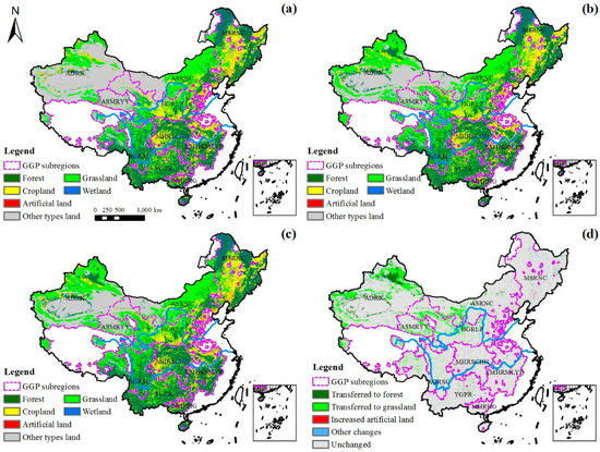
Figure 3. Spatial pattern of ecosystem distribution and transformation in the Grain for Green Program (GGP) area. (a–c) are the ecosystem distributions in 2010, 2005, and 2010, respectively; (d) is the ecosystem transformation from 2000 to 2010.

The LULC transfer matrix (Table 4) demonstrated that the interconversion of cropland and forest played a primary role in ecosystem pattern change during 2000–2010, with 2.45% of cropland converted to forest and 1.11% of forest transferred to cropland. In addition, the transformations from cropland to artificial land, from grassland to forest, from cropland to grassland, and from grassland to cropland were also significant. The ecosystem transformation mainly took place in 2005–2010, since the transformed area of each ecosystem type was almost twice as much as that from 2000 to 2005. Forest, grassland, and cropland ecosystems were the major transfer direction and sources to each other, while wetland was mainly converted to cropland and grassland and was also mainly replenished from cropland, grassland, and other types of land. Artificial land mostly came from and transferred into cropland. Among all ecosystems, the dynamics of wetland were the most drastic: only 96.54%, 95.76%, and 93.56% wetland remained unchanged during 2000–2005, 2005–2010, and 2000–2010, respectively. Wetland primarily transferred into cropland, which ranked second in ecosystem change intensity (94.10% unchanged in 2000–2010), followed by artificial land (95.43% unchanged), grassland (97.44% unchanged), forest (98.13% unchanged), and other types of land (99.19% unchanged). The ecosystem transformation to forest was scattered throughout the whole GGP, but concentrated in ADRX; while the ecosystem transformation to grassland mainly occurred in the northwestern GGP regions, including western HGRLP, ASMRYY, ADRX, and AGRSC. Artificial land mainly increased in the eastern GGP regions (Figure 3d).

Table 4. LULC transfer matrix of the Grain for Green Program (GGP) area from 2000–2010 (km²).

Period		Forest	Grassland	Wetland	Cropland	Artificial Land	Other Types Land
2000–2005	Forest	2,221,698	3377	721	6362	1021	318
	Grassland	7208	1,951,219	1971	7794	1457	797
	Wetland	559	1473	188,013	3369	424	912
	Cropland	11,774	10,866	2838	1,378,212	8637	515
	Artificial land	167	192	40	671	116,053	13
	Other types land	957	1867	1572	1240	667	1,482,015
2005–2010	Forest	2,207,645	9875	1649	20,204	1850	1126
	Grassland	16,861	1,931,738	2375	13,404	2608	2004
	Wetland	733	1731	186,901	4091	658	1054
	Cropland	23,784	10,651	3800	1,343,690	14,936	722
	Artificial land	489	442	177	4564	122,560	28
	Other types land	1233	2538	1766	1160	627	1,477,253
2000–2010	Forest	2,191,766	10310	2124	24,896	3136	1249
	Grassland	20,824	1,919,914	3632	19,848	3982	2241
	Wetland	1025	2489	182,188	6597	1053	1382
	Cropland	34,660	19,994	5752	1,329,406	21,975	989
	Artificial land	449	440	178	4258	111,770	33
	Other types land	2019	3829	2773	2107	1300	1,476,289

Note: Each row denotes the LULC transfer source, and each column denotes the LULC transfer destination.

3.2. Spatial Pattern and Temporal Trend of Ecosystem Quality

The terrestrial ecosystems in the GGP region from 2000 to 2010 had an average of 57.33%, 1.91, and 438.65 gC m⁻² in annual FVC_max, LAI_max, and NPP_avg, respectively (Table 5). The spatial patterns of EQ distribution and change are shown in Figure 4, and varied distinctly across the whole restoration area. Higher FVC_max, LAI_max, and NPP_avg values were distributed in the MHRHG, YGPR, MHRSCHH, LMHRMLYP, and MSRNC (roughly concentrated between 84%–94%, 3–4, and 700–1000 gC m⁻², respectively, all greater than the corresponding annual average value for the whole GGP region), over southern and northeastern China, where most forests are located. Northwestern China showed poor EQ, especially the HGRLP, ASRNC, ASMRYY, and ADRX, and the EQ and vegetated land descended in turn (Figure 4a–c and Figure 5). The spatial changes of annual FVC_max and LAI_max from 2000 to 2010 basically followed the same spatial pattern as distributions—gradually decreasing from southeast to northwest overall—but differed in some areas. For example, the eastern HGRLP, central and southwest of MSRNC, where lower FVC_max and LAI_max values were concentrated, had positive changes; the northwestern ADRX, where higher FVC_max and LAI_max values were found, however, was getting worse (Figure 4a,b,d,e). In relation to annual NPP_avg change, the slope declined from the center (eastern HGRLP and northern MHRSCHH) to the periphery in general, and the southern subregions suffered a more severe loss of NPP_avg, whereas the northern subregions had improved (Figure 4c,f).

Table 5. Statistical parameter values of ecosystem quality indicators in the Grain for Green Program (GGP) area from 2000 to 2010. The units of the mean and slope of FVC_max are % and % yr⁻¹, respectively; for NPP_avg, units are gC m⁻² and gC m⁻² yr⁻¹, respectively; and the LAI_max is dimensionless.

Ecosystem Quality	Subregions	Mean	Slope	R2	P
FVCmax	GGP	57.33	0.1459	0.3964	0.0379 *
	MSRNC	87.04	0.1197	0.0720	0.4249
	ASRNC	39.53	0.0376	0.0032	0.8689
	ADRX	17.61	−0.0280	0.0256	0.6385
	ASMRYY	28.78	0.1958	0.2889	0.0881
	HGRLP	49.41	0.5083	0.7244	0.0009 **
	AGRSC	69.68	0.0173	0.0101	0.7687
	MHRSCHH	91.23	0.2411	0.6404	0.0031 **
	LMHRMLYP	88.24	0.2681	0.4348	0.0273 *
	YGPR	91.21	0.2087	0.9210	0.0000 **
	MHRHG	91.90	0.3554	0.6707	0.0020 **
LAImax	GGP	1.91	0.0125	0.6753	0.0019 **
	MSRNC	3.63	0.0229	0.3613	0.0505
	ASRNC	0.87	0.0047	0.0490	0.5132
	ADRX	0.27	0.00003	0.0000	0.9851
	ASMRYY	0.57	0.0053	0.1297	0.2766
	HGRLP	1.24	0.0267	0.8028	0.0002 **
	AGRSC	2.06	0.0007	0.0008	0.9337
	MHRSCHH	3.46	0.0056	0.0750	0.4151
	LMHRMLYP	3.36	0.0270	0.6659	0.0022 **
	YGPR	3.52	0.0127	0.2961	0.0835
	MHRHG	3.45	0.0724	0.6408	0.0031 **
NPPavg	GGP	438.65	2.6958	0.1910	0.1790
	MSRNC	531.66	3.3390	0.1319	0.2722
	ASRNC	138.62	2.4287	0.1466	0.2452
	ADRX	33.78	−0.2360	0.0255	0.6388
	ASMRYY	62.16	1.3556	0.2036	0.1636
	HGRLP	209.77	8.0381	0.7951	0.0002 **
	AGRSC	337.02	−0.3149	0.0043	0.8487
	MHRSCHH	796.68	3.8604	0.0537	0.4928
	LMHRMLYP	834.41	7.1431	0.1574	0.2271
	YGPR	728.23	−2.1696	0.0247	0.6445
	MHRHG	920.48	1.7878	0.0065	0.8131

Note: the * symbol on the top-right of the P value means the tendency is significant (P < 0.05), and the ** symbol means the tendency is very significant (P < 0.01).

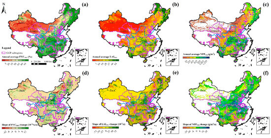
Figure 4. Spatial pattern of annual average ecosystem quality (EQ) and slope of EQ change in the Grain for Green Program (GGP) area from 2000 to 2010. (a–c) are the annual average FVC_max, LAI_max, and NPP_avg, respectively; (d–f) refer to the slope of annual FVC_max, LAI_max, and NPP_avg changes, respectively.

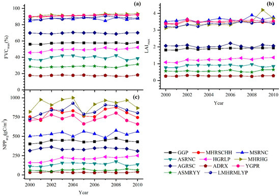
Figure 5. Temporal trends of annual ecosystem quality (EQ) changes in the Grain for Green Program (GGP) area from 2000 to 2010. (a–c) are the temporal trends of annual FVC_max, LAI_max, and NPP_avg changes, respectively.

There were significant temporal trends in changes in annual FVC_max and LAI_max over the whole GGP area from 2000 to 2010, reaching 0.1459% yr⁻¹ (R² = 0.3964, P < 0.05) and 0.0121 yr⁻¹ (R² = 0.6672, P < 0.01), respectively, although this was not so for the NPP_avg, which reached 2.6958 gC m⁻² yr⁻¹ (R² = 0.1910, P > 0.05) (Figure 5, Table 5). The annual FVC_max, LAI_max, and NPP_avg changes, in general, all showed a slightly increasing trend in the decade, indicating that the EQ of the restoration region had improved. Large variations in the temporal trends of annual FVC_max, LAI_max, and NPP_avg existed across the whole GGP region (Figure 5, Table 5). The annual FVC_max and LAI_max in most subregions remained basically stable with minor fluctuations and an overall slight increase, except FVC_max in ADRX and LAI_max in MHRHG. The increase in annual FVC_max mainly occurred in HGRLP, with the highest rate of 0.5083% yr⁻¹(R² = 0.7244, P < 0.01), followed by MHRHG, LMHRMLYP, MHRSCHH, and YGPR, with significant slopes of over 0.2% yr⁻¹ (P < 0.05) (Figure 4d and Figure 5a). The annual LAI_max mainly increased in MHRHG, with the highest slope of 0.0724 yr⁻¹ (R² = 0.6425, P < 0.01), followed by LMHRMLYP and HGRLP, with slopes of over 0.02 yr⁻¹ (P < 0.01). The EQ in these three regions rose very significantly (Figure 4e and Figure 5b). The annual NPP_avg change showed relatively large fluctuations in the MHRHG, LMHRMLYP, MHRSCHH, and YGPR, but oscillated with micro amplitudes in other subregions. The annual NPP_avg in most subregions rose in general, especially in the HGRLP (with the highest slope of 8.0381 gC m⁻² yr⁻¹, R² = 0.7950, P < 0.01), LMHRMLYP, MHRSCHH, and MSRNC, while the annual NPP_avg in the ADRX, AGRSC, and YGPR decreased (Figure 4f and Figure 5c).

3.3. Spatial Pattern and Temporal Trend of Key Ecosystem Services

The annual WR, SWAL, and SWIL were estimated to be 108.76 × 10⁴ t km⁻², 15.62 t ha, and 16.58 t ha per unit area per year, respectively, at total quantities of 580.56 billion tons, 11.57 billion tons, and 12.27 billion tons in the whole GGP area from 2000 to 2010 (Table 6). Figure 6 demonstrates that all the three key ESs displayed great spatial heterogeneity in distribution, with the southeast subregions generally performing much better than the northwest. The annual WR_pua decreased gradually from southeast to northwest, while the annual SWAL_pua increased from northeast to southwest in total, and the SWIL basically occurred in Northwest China (Figure 6a–c). With respect to spatial changes of ESs, the southern subregions, which contained most of the WR owing to abundant precipitation and high vegetation cover, showed weaker WR from 2000 to 2010, while the northern subregions with poor WR showed a positive trend (Figure 6a,d). Soil water erosion was alleviated effectively all over the GGP region, especially in the HGRLP, AGRSC, and YGPR, where the severest SWAL occurred due to the Loess Plateau and alpine valleys, but the situation remained poor in the southern edges of the ADRX and ASMRYY (Figure 6b,e). It was gratifying that positive changes in soil wind erosion had also occurred in the regions with heavy SWIL, i.e., the middle of the ADRX and western ASRNC, but in some regions—the northwest of ASMRYY and HGRLP—the deterioration continued. It should be noted that a slight increase in soil wind erosion appeared in a few areas which seldom had SWIL (eastern ASRNC and parts of south subregions) (Figure 6c,f).

Table 6. Statistical parameters of ecosystem services indicators in the Grain for Green Program (GGP) area from 2000 to 2010. The units of the mean and slope of WR_pua are 10⁴ t km⁻² and 10⁴ t km⁻² yr⁻¹, respectively, while for both SWAL_pua and SWIL_pua, units are t ha and t ha yr⁻¹, respectively.

Ecosystem Services	Subregions	Mean	Slope	R2	P
WRpua	GGP	108.76	−0.2283	0.0176	0.6978
	MSRNC	125.35	0.4587	0.0629	0.4570
	ASRNC	30.08	0.0473	0.0044	0.8457
	ADRX	27.65	−0.3970	0.2472	0.1197
	ASMRYY	63.31	0.2047	0.0744	0.4172
	HGRLP	41.70	0.2916	0.0593	0.4706
	AGRSC	147.61	−1.0921	0.0964	0.3527
	MHRSCHH	141.33	0.7153	0.0393	0.5592
	LMHRMLYP	214.32	−0.3466	0.0016	0.9066
	YGPR	187.11	−1.8224	0.1084	0.3228
	MHRHG	246.66	−0.0342	0.0000	0.9931
SWALpua	GGP	15.62	−0.0841	0.0251	0.6420
	MSRNC	2.37	0.1407	0.2696	0.1017
	ASRNC	5.25	−0.0611	0.0685	0.4367
	ADRX	11.80	0.6213	0.2194	0.1462
	ASMRYY	20.70	0.0420	0.0010	0.9253
	HGRLP	18.78	−0.7505	0.6079	0.0047 **
	AGRSC	56.93	−0.3829	0.0635	0.4546
	MHRSCHH	9.96	−0.3343	0.3447	0.0575
	LMHRMLYP	7.51	−0.1435	0.0333	0.5914
	YGPR	21.76	−0.9375	0.3746	0.0453 *
	MHRHG	10.44	−0.1267	0.0165	0.7069
SWILpua	GGP	16.58	−1.0071	0.4570	0.0224 *
	MSRNC	3.24	−0.3714	0.6288	0.0036 **
	ASRNC	41.51	−1.5977	0.2511	0.1163
	ADRX	36.08	−3.4267	0.5883	0.0059 **
	ASMRYY	24.06	0.0445	0.0005	0.9497
	HGRLP	12.28	0.1235	0.0134	0.7350
	AGRSC	0.61	−0.0583	0.6016	0.0050 **
	MHRSCHH	0.01	−0.0008	0.2652	0.1050
	LMHRMLYP	0.03	−0.0029	0.5356	0.0105 *
	YGPR	0.02	−0.0005	0.0086	0.7868
	MHRHG	0.39	−0.0021	0.0027	0.8796

Note: the * symbol on the top-right of the P value means the tendency is significant (P < 0.05), and the ** symbol means the tendency is very significant (P < 0.01).

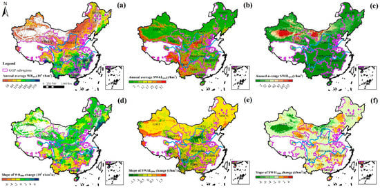
Figure 6. Spatial pattern of annual average ecosystem services (ESs) and slope of ESs change in the Grain for Green Program (GGP) area from 2000–2010. (a–c) are the annual average WR_pua, SWAL_pua, and SWIL_pua, respectively; (d–f) refer to the slope of annual WR_pua, SWAL_pua, and SWIL_pua changes, respectively.

Unlike EQ, the temporal trends of the three key ESs were not very significant. The slopes of annual WR_pua, SWAL_pua, and SWIL_pua changes were −2283 t km⁻² yr⁻¹, −0.0841 t ha yr⁻¹, and −1.0071 t ha yr⁻¹, respectively (R² = 0.4570, P < 0.05) (Figure 7, Table 6). The declines in SWAL_pua and SWIL_pua implied that the ESs of SC and SP in the GGP area from 2000 to 2010 had been enhanced overall (especially SP), whereas the improvement of WR was not reflected clearly and tended to exhibit a slight weakening. However, the temporal trend of ESs on the subregion-scale differed from the whole region, especially the WR_pua. Half of the subregions, mostly in the north, appeared to show steady rises. In the southern subregions, the annual WR_pua decreased overall, with obvious fluctuations (Figure 7a, Table 6). With 56.93 t ha on average, the annual SWAL_pua in AGRSC was about two to 24 times higher than any other subregions and had much bigger fluctuations. The annual SWAL_pua dropped with minor fluctuations in most areas, and significantly in the YGPR (P < 0.05) and HGRLP (P < 0.01), although there was an increase in three northern subregions: ADRX, MSRNC, and ASMRYY (Figure 7b, Table 6). The annual SWIL_pua decreased very significantly in ADRX (P < 0.01), MSRNC (P < 0.01), AGRSC (P < 0.01), and LMHRMLYP (P < 0.05); while that in ASRNC, HGRLP, and ASMRYY showed a downward trend at first, but later an upward trend; and HGRLP and ASMRYY eventually rose slightly on the whole (Figure 7c, Table 6). The annual WR_pua, SWAL_pua, and SWIL_pua in ASMRYY all showed rising trends, which were the opposite to those in the whole GGP area.

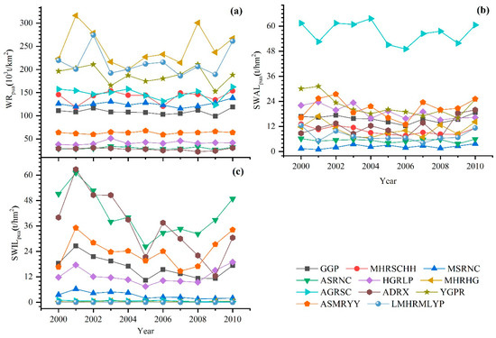
Figure 7. Temporal trends of annual ecosystem services (ESs) changes in the Grain for Green Program (GGP) area from 2000 to 2010. (a–c) are the temporal trends of annual WR_pua, SWAL_pua, and SWIL_pua changes, respectively.

4. Discussion

4.1. Trade-Offs and Synergies of Ecological Indicators in GGP Area

Large trade-offs have occurred between ecosystem services, largely due to land-use and land management changes [75]. Combining multiple ecological outputs under the scenario of GGP demonstrates the extent of the tradeoffs or synergies among these ecological variables. In the whole GGP region, most pair-wise ecological indicators were revealed to be remarkably correlated (Figure 8). FVC, LAI, and NPP showed a strong and significant positive correlation with each other (P < 0.05), presenting synergies among EQ variables. With respect to ESs, WR positively correlated with SWAL (P < 0.05), indicating a remarkable trade-off with SC. The relatively positive correlation between SWIL and WR and between SWIL and SWAL, implied a trade-off between SP and WR and a synergy between SP and SC. While SWAL and SWIL were negatively correlated with relative EQ indicators, presenting synergies of ESs of SC and SP with EQ, WR showed no apparent tendency with EQ. Since the FVC and LAI respectively parameterize the horizontal and vertical density of vegetation [31], and NPP is the rate of net accumulation of organic matter in plants [76], with the growth of vegetation, they increase simultaneously in general. Vegetation generally reduces runoff and soil water erosion and thus enhances soil retention by intercepting rainfall, increasing water infiltration, increasing soil shear strength, reducing raindrop energy and ‘splash’ effects, and trapping sediment where rainfall is abundant [77,78,79], and halts near-surface sand flow, hence improving sand fixation by stabilizing soil, increasing underlying surface roughness, reducing near-surface wind speed, and weakening sand transportation intensity in arid and semi-arid regions [80,81,82].

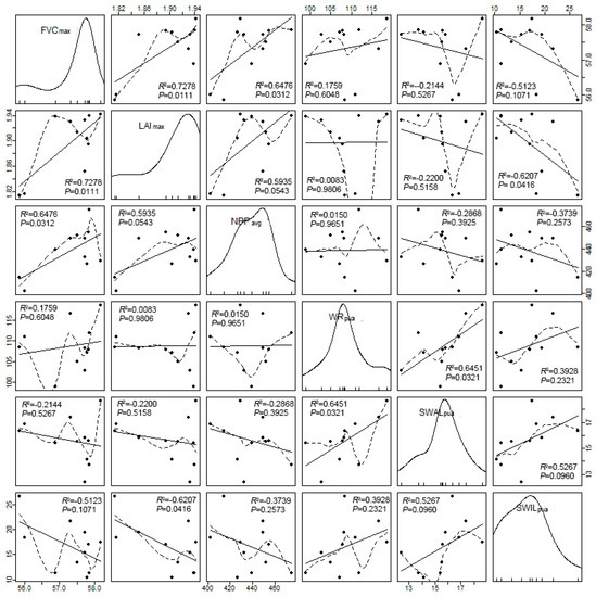
Figure 8. Tradeoffs and synergies among variables of EQ and ESs.

Our findings of no apparent tendency between WR and EQ seemed to be slightly different from the discovery of Jia et al. [23], who reported that the water yield in North Shaanxi showed no apparent tendency with NPP, but declined with the increase of biomass after eight years of GGP implementation, and contrary to Cao et al [83] and Feng et al [26], who claimed that there was a trade-off between the water yield and afforestation in the Loess Plateau. These might be attributable to the larger scale of our study area. The relationship between a pair of ESs can differ across different scales and across different socio-ecological systems [84,85]. The whole GGP region represented vast spatial heterogeneity of natural characteristics and climate, while the previous work focused on arid or semi-arid areas. Due to the fact that the debate about the balance of benefits and disbenefits of forestry in water regulation is still widespread around the planet [86,87,88,89], the effects of climate and geographic locations on water conservation need further consideration.

4.2. Impact of Climate Change on Ecological Change in the GGP Subregions

Climate variability and ecological restoration programs jointly influence vegetation growth [78], thus further impacting EQ and ESs. From 2000 to 2010, the climate in the whole GGP area became warmer and wetter, with average increments of 0.0292 °C and 0.4685 mm per year in temperature and precipitation, respectively. Climate change showed large spatial heterogeneity, with wetter places (mainly southern subregions) becoming drier, and drier places (mainly northern subregions) becoming wetter. Most of the southern and northwestern subregions became warmer, especially in the southwest, while central and northeast subregions became colder (Figure 9). We used the slope of annual FVC_max, LAI_max, NPP_avg, WR_pua, SWAL_pua, and SWIL_pua changes and the slope of annual precipitation and temperature changes to investigate the relationship between the ecological changes and climate change at a subregion scale (Figure 10). We found that the impacts of precipitation and temperature on ecological changes at a subregion level were not significant, except WR_pua, which was impacted by precipitation very significantly (R² = 0.78, P < 0.01) (Figure 10d). Therefore, the increase in precipitation might explain the rise of WR_pua in most northern subregions, while the decrease led to a decline in WR_pua in most southern subregions. However, the WR_pua and precipitation of subregions did not fluctuate with the same volatility and the response of WR_pua to precipitation change in northern subregions was weaker than that in southern subregions, e.g., the slope values for precipitation change in the ASRNC, HGRLP, and MHRSCHH were similar, but the slopes for WR_pua change in the ASRNC and HGRLP were far lower than in MHRSCHH (Figure 10d). Considering the abnormal rise of annual FVC_max, LAI_max, and NPP_avg compared with climate change in northern subregions, especially in the HGRLP (Figure 10a–c), the increased forest might lead to a reduction in the water yield in arid and semi-arid regions [78,83,90], whereas the precipitation might become a more constraining factor to water conservation in humid areas. New planting would increase ET and induce a significant decrease in the ratio of river runoff to annual precipitation across hydrological catchments [26], and large-scale afforestation in vulnerable arid and semi-arid regions could increase the severity of water shortages [83]. Besides WR_pua, the SWIL_pua in the ASMRYY and HGRLP still increased slightly under the scenarios of afforestation (Figure 10f), concurring with the discovery of Cao [22], who found that planting trees in arid and semi-arid regions had failed to mitigate desertification. The correlation was relatively high between SWAL_pua and precipitation (Figure 10e), indicating that climate change contributes to the enhancement of SC. The fact that the effects of climate change on most ecological variables at a subregion level were not significant implied that the GGP might play a more important role in ecological change, and the difference of ecological outputs among subregions might be attributed to different regional restoration measures (Table 1). The selection and richness of tree species, area, and locations for revegetation or afforestation would significantly influence the ecological effects [91,92].

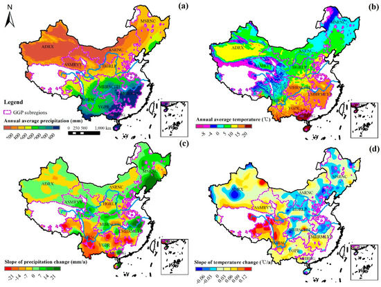
Figure 9. Spatial pattern of annual average climate and slope of climate change in the Grain for Green Program (GGP) area from 2000 to 2010. (a,b) are the annual average precipitation and temperature, respectively; (c,d) refer to the slope of annual precipitation and temperature changes, respectively.

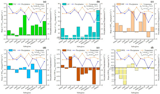
Figure 10. Relationship between the difference in ecological changes among Grain for Green Program (GGP) subregions and climate condition from 2000 to 2010. (a–f) are the slope of annual FVC_max, LAI_max, NPP_avg, WR_pua, SWAL_pua, and SWIL_pua changes compared with the slope of annual precipitation and temperature changes from 2000 to 2010, respectively.

4.3. The Contribution of the GGP Implementation to Ecological Change

Climate change can enhance the ecological condition to some extent, but the GGP only affected new vegetation in the GGP area. To find out the contribution of GGP implementation to the ecological benefit, a paired Welch’s t-test was conducted to compare the slope of annual FVC_max, LAI_max, NPP_avg, WR_pua, SWAL_pua, and SWIL_pua changes between two LULC types: (1) the restored vegetation (including forest and grassland) transferred from another LULC type from 2000 to 2010 (LULC A); and (2) the retained forest and grassland that existed before 2000 and remained untransformed from 2000 to 2010 (LULC B). The sample points of LULC A (denoted as Sample A) were selected from the pixels that were transferred to forest and grassland in 2000–2010 at a 1 km spatial resolution. The sample points of LULC B (denoted as Sample B) were randomly selected from the intersecting pixels of forest and grassland in the 2000, 2005, and 2010 LULC dataset in the nearest neighborhood of Sample A, to ensure similar climate conditions and further exclude the influence of climate change. Both samples had about 15000 points, involving 56% forest and 44% grassland. The null hypothesis and alternative hypothesis are listed in Table 7. Results showed that the slope of annual FVC_max, LAI_max, NPP_avg, and SWAL_pua changes passed the paired Welch’s t-test at a very significant level, whereas the slope of annual precipitation and temperature changes did not, indicating that the recovery/improvement rates of EQ and SC in the revegetation area were higher than existing vegetation under similar climate conditions. Therefore, the GGP implementation rather than climatic change was the primary cause for the estimated increase of ecosystem quality and services, which is supported by many studies [15,19,26]. The slope of annual FVC_max, LAI_max, and NPP_avg changes in LULC A increased by 14.23%, 9.94%, and 8.23%, respectively, compared with those in LULC B, while the slope of annual SWAL_pua change in LULC A decreased by 30.45% compared with LULC B. This change should be considered as the contribution of the GGP implementation.

Table 7. Null hypothesis and alternative hypothesis for the slope of changes of climate, ecosystem quality, and ecosystem services indicator values between Sample A and Sample B from 2000 to 2010. μ_A and μ_B are, respectively, the mean of the slope value of Sample A and Sample B, and the units from top to bottom are mm yr⁻¹, °C yr⁻¹, % yr⁻¹, yr⁻¹, gC m⁻² yr⁻¹, 10⁴ t km⁻² yr⁻¹, t ha yr⁻¹, and t ha yr^−1.

Slope	Null Hypothesis (H0)	Alternative Hypothesis (H1)	μA	μB	P
Precipitation	μA = μB	μA ≠ μB	−1.6727	−1.7462	0.5230
Temperature	μA = μB	μA ≠ μB	0.0212	0.0214	0.5496
FVCmax	μA = μB	μA > μB	0.0059	0.0052	<0.0001 **
LAImax	μA = μB	μA > μB	0.0269	0.0245	0.0002 **
NPPavg	μA = μB	μA > μB	4.9719	4.5936	0.0019 **
WRpua	μA = μB	μA > μB	0.0207	0.0184	0.3504
SWALpua	μA = μB	μA < μB	−1.4246	−1.0921	<0.0001 **
SWILpua	μA = μB	μA < μB	−0.1212	−0.1160	0.2087

Note: the * symbol on the top-right of the P value means the tendency is significant (P < 0.05), for ** symbol means the tendency is very significant (P < 0.01).

As the slope of annual WR_pua and SWIL_pua changes did not pass the t-test, we further conducted paired Welch’s t-tests on them between LULC A and LULC B in forest and grassland separately, and found that the slope of SWIL_pua in restored grassland passed the t-test with high significance and it decreased by 18.05% more than that in LULC B grassland (μ_A = −0.2260, μ_B = −0.1914, P < 0.01). The slope of annual SWIL_pua change in restored forest and the slope of annual WR_pua change in neither restored forest nor grassland did not pass the t-test. The results further confirmed our findings in the last section. Afforestation with inappropriate species in arid and semi-arid regions can damage local water balances because of the high consumption of plant transpiration and evaporation from the soil surface [93,94], and thus aggravate water shortages and soil degradation [95], leading to erosion and further exacerbating desertification in the long term [89]. In this case, introducing stable communities of natural desert steppe and grassland vegetation is a more appropriate way to sustain the natural ecosystem and control the spread of desertification [96].

4.4. Implications for the New Round of the GGP

To investigate the gap between new plantings and retained vegetation in improving ecological conditions, a paired Welch’s t-test was conducted to compare the annual average FVC_max, LAI_max, NPP_avg, WR_pua, SWAL_pua, and SWIL_pua between LULC A and LULC B from 2000 to 2010. The null hypothesis and alternative hypothesis are listed in Table 8. All the indicators except SWIL_pua passed the t-test at a very significant level. The annual average FVC_max, LAI_max, NPP_avg, and WR_pua in LULC A were respectively 2.56%, 6.74%, 8.81%, and 22.34% less than those in LULC B, and the annual average SWAL_pua and SWIL_pua were respectively 7.39% and 5.22% higher than those in LULC B, suggesting that the new planting had not reached its potential maximum in terms of ecosystem condition enhancement. Therefore, as the new round of GGP is initiated, more attention should be paid to the protection and restoration of old-growth original forest, the cultivation of young planted forest, and the management of artificial forests, apart from only afforestation and reforestation. To achieve this goal, besides the institutional arrangements such as legislation, setting up nature reserves and enhancing incentive payments, which the government always does, market tools, the development of new technology, and international programs should be taken into account. Responsible forest management could be promoted by bringing in market-based third-party certification for evaluating forests according to a set of standards [97,98]. Improving the biological, physiological, and genetic quality of forest planting stock through plant biotechnology, a high level of environmental control in the growth chambers, and transnational co-operation are also practical ways to carry out forest restoration projects [99,100,101,102]. International climate change mitigation programs, which are designed to reduce emissions from deforestation and forest degradation in developing countries (REDD+), should also be taken into consideration as collateral payments for the substantial carbon benefit in maintaining forest [103].

Table 8. Null hypothesis and alternative hypothesis of mean annual values of ecosystem quality and ecosystem services indicators between Sample A and Sample B from 2000–2010. μ_A and μ_B are, respectively, the mean of annual values of indicators of Sample A and Sample B, and the units from top to bottom are %, dimensionless, gC m⁻², 10⁴ t km⁻², t ha, and t ha.

Mean	Null Hypothesis (H0)	Alternative Hypothesis (H1)	μA	μB	P
FVCmax	μA = μB	μA < μB	75.1732	77.1498	<0.0001 **
LAImax	μA = μB	μA < μB	2.3096	2.4766	<0.0001 **
NPPavg	μA = μB	μA < μB	410.8583	450.5745	<0.0001 **
WRpua	μA = μB	μA < μB	8.9232	11.4906	<0.0001 **
SWALpua	μA = μB	μA > μB	20.9982	19.5538	<0.0001 **
SWILpua	μA = μB	μA > μB	1.4887	1.4148	0.1046

Note: the * symbol on the top-right of the P value means the tendency is significant (P < 0.05), and the ** symbol means the tendency is very significant (P < 0.01).

Our studies suggested that not all the ESs increased simultaneously under the scenario of reforestation and afforestation, and significant differences and lags existed between the improvement of each pair of ecological indicators. This implied the existence of trade-offs and synergies between ESs, which complicates the restoration mechanism and must be considered in policy-making [19,23]. Considering the more important role GGP played in ecological change and the variation of ecological change among subregions, regional restoration measures need to be concerned carefully. More attention should be paid to re-establishing near-natural forests or the restoration of a region’s natural climax vegetation [22,96,104,105,106].

Owing to the urgent need to address eco-environmental problems, the Chinese government had to act before the achievement of scientific consensus, which needs a step-by-step investigation and does not provide instant solutions [107]. Therefore, the massive afforestation program which ignored differences in topography, climate, and hydrology in the first round of the GGP is understandable. In future GGP policy-making and implementation, we suggest that the former practice of aggressive afforestation on a large-scale must be changed. Rational and specific plans and designs for afforestation areas should seek scientific advice before implementation according to regional climate and geographical characteristics, including local temperatures, precipitation, terrain, soil, and hydrology. In addition to the appropriateness of tree species, near-natural vegetation communities which take into account diversity and mixtures of the tree-shrub-herb system should be planted instead of single-species plantations.

References

- Liu, J.G.; Diamond, J. China’s environment in a globalizing world. Nature 2005, 435, 1179–1186. [Google Scholar] [CrossRef] [PubMed]
- Zhang, P.; Shao, G.; Zhao, G.; Le Master, D.C.; Parker, G.R.; Dunning, J.B.; Li, Q. Ecology-China’s forest policy for the 21st century. Science 2000, 288, 2135–2136. [Google Scholar] [CrossRef] [PubMed]
- Fan, J.W.; Zhong, H.P.; Yuan, X.J. Natural grassland reclamation and its ecological impaction in recent 50 years. Grassl. China 2002, 24, 70–73. (In Chinese) [Google Scholar] [CrossRef]
- Xu, Z.G.; Xu, J.T.; Deng, X.Z.; Huang, J.K.; Uchida, E.; Rozelle, S. Grain for Green versus Grain: Conflict between food security and conservation set-aside in China. World Dev. 2006, 34, 130–148. [Google Scholar] [CrossRef]
- He, F.N.; Ge, Q.S.; Dai, J.H.; Rao, Y.J. Forest change of China in recent 300 years. J. Geogr. Sci. 2008, 18, 59–72. [Google Scholar] [CrossRef]
- Shi, H.; Shao, M. Soil and water loss from the Loess Plateau in China. J. Arid Environ. 2000, 45, 9–20. [Google Scholar] [CrossRef]
- Wang, T.; Zhu, Z. Study on Sandy Desertification in China. J. Des. Res. 2003, 23, 209–214. [Google Scholar]
- Wang, X.; Lu, C.; Fang, J.; Shen, Y. Implications for development of grain-for-green policy based on cropland suitability evaluation in desertification-affected north China. Land Use Policy 2007, 24, 417–424. [Google Scholar] [CrossRef]
- Li, J.; Zhao, J.; Chen, H. Threats to biodiversity in China and countermeasures. J. Northwest Sci-Tech Univ. Agric. For. 2003, 31, 158–162. (In Chinese) [Google Scholar] [CrossRef]
- Jiang, Z.; Jiang, J.; Wang, Y.; Zhang, E.; Zhang, Y.; Li, L.; Cai, B.; Luo, Z.; Li, C.; Ping, X.; et al. China’s ecosystems: Overlooked species. Science 2016, 353, 657. [Google Scholar] [CrossRef] [PubMed]
- Li, W. Flood of Yangtze River and ecological restoration. J. Nat. Resour. 1999, 14, 1–8. (In Chinese) [Google Scholar] [CrossRef]
- Lu, S.; Huang, X.; Li, S.; Wang, Y.; Zhang, Y. The systematic analysis of reclamation of arable land for reforestation. Hebei J. For. Orch. Res. 2003, 18, 20–23. (In Chinese) [Google Scholar]
- Sun, D.F.; Li, H.; Dawson, R.; Tang, C.J.; Li, X.W. Characteristics of steep cultivated land and the impact of the Grain-for-Green Policy in China. Pedosphere 2006, 16, 215–223. [Google Scholar] [CrossRef]
- Chokkalingam, U.; Zhou, Z.; Wang, C.; Takeshi, T. Learning Lessons from China’s Forest Rehabilitation Efforts: National Level Review and Special Focus on Guangdong Province; SMK Grafika Desa Putera: Jakarta, Indonesia, 2006. [Google Scholar]
- Deng, L.; Liu, G.; Shangguan, Z. Land-use conversion and changing soil carbon stocks in China’s ‘Grain-for-Green’ Program: A synthesis. Glob. Change Biol. 2014, 20, 3544–3556. [Google Scholar] [CrossRef] [PubMed]
- Yin, R.; Yin, G. China’s primary programs of terrestrial ecosystem restoration: Initiation, implementation, and challenges. Environ. Manag. 2010, 45, 429–441. [Google Scholar] [CrossRef]
- Xie, C.; Wang, J.; Peng, W.; Zhang, K.; Liu, J.; Yu, B.; Jiang, X. The New Round of CCFP: Policy Improvement and Implementation Wisdom. For. Econ. 2016, 43–51. (In Chinese) [Google Scholar] [CrossRef]
- Xinhua News Agency. The Country Has Invested More Than 4000 Billion Yuan for The First Round of Grain for Green Program. Available online: http://news.xinhuanet.com/politics/2015-08/07/c_1116185623.htm (accessed on 20 July 2018). (In Chinese).
- Wang, J.; Peng, J.; Zhao, M.; Liu, Y.; Chen, Y. Significant trade-off for the impact of Grain-for-Green Programme on ecosystem services in North-western Yunnan, China. Sci. Total Environ. 2017, 574, 57–64. [Google Scholar] [CrossRef]
- Feng, Z.; Yang, Y.; Zhang, Y.; Zhang, P.; Li, Y. Grain-for-green policy and its impacts on grain supply in West China. Land Use Policy 2005, 22, 301–312. [Google Scholar] [CrossRef]
- Fu, B.; Hu, C.; Chen, L.; Honnay, O.; Gulinck, H. Evaluating change in agricultural landscape pattern between 1980 and 2000 in the Loess hilly region of Ansai County, China. Agric. Ecosyst. Environ. 2006, 114, 387–396. [Google Scholar] [CrossRef]
- Cao, S. Why large-scale afforestation efforts in China have failed to solve the desertification problem. Environ. Sci. Technol. 2008, 42, 1826–1831. [Google Scholar] [CrossRef]
- Jia, X.; Fu, B.; Feng, X.; Hou, G.; Liu, Y.; Wang, X. The tradeoff and synergy between ecosystem services in the Grain-for-Green areas in Northern Shaanxi, China. Ecol. Indic. 2014, 43, 103–113. [Google Scholar] [CrossRef]
- Zhu, J.X.; Wang, J.L. Study on Grain for Green Project implementation effect monitoring based on high resolution image: A case Study in Ansai County, Shanxi Province, China. In Proceedings of the 21st International Conference on Geoinformatics, Kai Feng, China, 20 June–22 June 2013; IEEE: New York, NY, USA, 2013. [Google Scholar]
- Li, H.; Cai, Y.; Chen, R.; Chen, Q.; Yan, X. Effect assessment of the project of grain for green in the karst region in Southwestern China: A case study of Bijie Prefecture. Acta Ecol. Sinica 2011, 31, 3255–3264. (In Chinese) [Google Scholar]
- Feng, X.; Fu, B.; Piao, S.; Wang, S.; Ciais, P.; Zeng, Z.; Lü, Y.; Zeng, Y.; Li, Y.; Jiang, X.; Wu, B. Revegetation in China’s Loess Plateau is approaching sustainable water resource limits. Nat. Clim. Change 2016, 11, 1019–1022. [Google Scholar] [CrossRef]
- China sustainable forestry strategy research project team. Research on Forestry Strategy of Sustainable Development in China: Strategic Volume; China Forestry Publishing House: Beijing, China, 2003. (In Chinese) [Google Scholar]
- Pettorelli, N.; Vik, J.O.; Mysterud, A.; Gaillard, J.M.; Tucker, C.J.; Stenseth, N.C. Using the satellite-derived NDVI to assess ecological responses to environmental change. Trends Ecol. Evol. 2005, 20, 503–510. [Google Scholar] [CrossRef] [PubMed]
- Jing, X.; Yao, W.; Wang, J.; Sonb, X. A study on the relationship between dynamic change of vegetation coverage and precipitation in Beijing’s mountainous areas during the last 20 years. Math Comput. Model. 2011, 54, 1079–1085. [Google Scholar] [CrossRef]
- Cowling, S.A.; Field, C.B. Environmental control of leaf area production: Implications for vegetation and land-surface modeling. Glob. Biogeochem. Cycles 2003, 17, 1007. [Google Scholar] [CrossRef]
- Gutman, G.; Ignatov, A. The derivation of the green vegetation fraction from NOAA/AVHRR data for use in numerical weather prediction models. Int. J. Remote Sens. 1998, 19, 1533–1543. [Google Scholar] [CrossRef]
- Breda, N.J.J. Ground-based measurements of leaf area index: A review of methods, instruments and current controversies. J. Exp. Bot. 2003, 54, 2403–2417. [Google Scholar] [CrossRef] [PubMed]
- Godinez-Alvarez, H.; Herrick, J.E.; Mattocks, M.; Toledo, D.; Van Zee, J. Comparison of three vegetation monitoring methods: Their relative utility for ecological assessment and monitoring. Ecol. Indic. 2009, 9, 1001–1008. [Google Scholar] [CrossRef]
- Zhang, X.; Liao, C.; Li, J.; Sun, Q. Fractional vegetation cover estimation in arid and semi-arid environments using HJ-1 satellite hyperspectral data. Int. J. Appl. Earth Obs. 2013, 21, 506–512. [Google Scholar] [CrossRef]
- Running, S.W.; Nemani, R.R.; Heinsch, F.A.; Zhao, M.S.; Reeves, M.; Hashimoto, H. A continuous satellite-derived measure of global terrestrial primary production. BioScience 2004, 54, 547–560. [Google Scholar] [CrossRef]
- Crabtree, R.; Potter, C.; Mullen, R.; Sheldon, J.; Huang, S.; Harmsen, J.; Rodman, A.; Jean, C. A modeling and spatio-temporal analysis framework for monitoring environmental change using NPP as an ecosystem indicator. Remote Sens. Environ. 2009, 113, 1486–1496. [Google Scholar] [CrossRef]
- Gower, S.T.; Kucharik, C.J.; Norman, J.M. Direct and indirect estimation of leaf area index, fAPAR, and net primary production of terrestrial ecosystems. Remote Sens. Environ. 1999, 70, 29–51. [Google Scholar] [CrossRef]
- Gregorio, A.D.; Jansen, L.J.M. Land Cover Classification System: Classification concepts and user manual for software version (2), 2nd ed.; Food and Agriculture Organization of the United Nations: Rome, Italy, 2005. [Google Scholar]
- Zhang, L.; Wu, B.; Li, X.; Xing, Q. Classification system of China land cover for carbon budget. Acta Ecol. Sinica 2014, 34, 7158–7166. (In Chinese) [Google Scholar] [CrossRef]
- Watson, R.T.; Noble, I.R.; Bolin, B.; Ravindranath, N.H.; Verardo, D.J.; Dokken, D.J. Land use, Land-Use change and forestry. Spec. Rep. IPCC 2000, 4, 375. [Google Scholar]
- Wu, B.; Yuan, Q.; Yan, Z.; Wang, Z.; Yu, X.; Li, A.; Ma, R.; Huang, J.; Chen, J.; Chang, C.; et al. Land cover changes of China from 2000 to 2010. Quat. Sci. 2014, 34, 723–731. (In Chinese) [Google Scholar] [CrossRef]
- Song, X.; Yan, Z. Land cover change detection using segment similarity of spectrum vector based on knowledge base. Acta Ecol. Sinica 2014, 34, 7175–7180. (In Chinese) [Google Scholar] [CrossRef]
- Xian, G.; Homer, C.; Fry, J. Updating the 2001 National Land Cover Database land cover classification to 2006 by using Landsat imagery change detection methods. Remote Sens. Environ. 2009, 113, 1133–1147. [Google Scholar] [CrossRef]
- Ouyang, Z.; Zhang, L.; Wu, B.; Li, X.; Xu, W.; Xiao, Y.; Zheng, H. An ecosystem classification system based on remote sensor information in China. Acta Ecol. Sinica 2015, 35, 219–226. (In Chinese) [Google Scholar] [CrossRef]
- Qiao, W.; Sheng, Y.; Fang, B.; Wang, Y. Land use change information mining in highly urbanized area based on transfer matrix: A case study of Suzhou, Jiangsu Province. Geogr. Res. 2013, 32, 1497–1507. (In Chinese) [Google Scholar]
- Jiapaer, G.; Chen, X.; Bao, A. A comparison of methods for estimating fractional vegetation cover in arid regions. Agric. For. Meteorol. 2011, 151, 1698–1710. [Google Scholar] [CrossRef]
- Holben, B.N. Characteristics of maximum-value composite images from temporal AVHRR data. Int. J. Remote Sens. 1986, 7, 1417–1434. [Google Scholar] [CrossRef]
- Savitzky, A.; Golay, M.J.E. Smoothing and differentiation of data by simplified least squares procedures. Anal. Chem. 1964, 36, 1627–1639. [Google Scholar] [CrossRef]
- Fang, H.; Liang, S.; Townshend, J.R.; Dickinson, R.E. Spatially and temporally continuous LAI data sets based on an integrated filtering method: Examples from North America. Remote Sens. Environ. 2008, 112, 75–93. [Google Scholar] [CrossRef]
- Wang, J.; Liu, J.; Shao, Q.; Liu, R.; Fan, J.; Chen, Z. Spatial-temporal patterns of net primary productivity for 1988-2004 based on GLOPEM-CEVSA model in the “Three-River Headwaters” Region of Qinghai Province, China. Chin. J. Plant Ecol. 2009, 33, 254–269. (In Chinese) [Google Scholar]
- Allen, R.G.; Pereira, L.S.; Raes, D.; Smith, M. Crop Evapotranspiration-Guidelines for Computing Crop Water Requirements-FAO Irrigation and Drainage Paper 56; Food and Agriculture Organization of the United Nations: Rome, Italy, 1998. [Google Scholar]
- Liu, R.; Chen, J.M.; Liu, J.; Deng, F.; Sun, R. Application of a new leaf area index algorithm to China’s landmass using MODIS data for carbon cycle research. J. Environ. Manag. 2007, 85, 649–658. [Google Scholar] [CrossRef] [PubMed]
- Cao, M.; Prince, S.D.; Small, J.; Goetz, S.J. Remotely sensed interannual variations and trends in terrestrial net primary productivity 1981–2000. Ecosystems 2004, 7, 233–242. [Google Scholar] [CrossRef]
- Hutchinson, M.F. Interpolating mean rainfall using thin plate smoothing splines. Int. J. Geogr. Inf. Syst. 1995, 9, 385–403. [Google Scholar] [CrossRef]
- Apaydin, H.; Sonmez, F.; Yildirim, Y. Spatial interpolation techniques for climate data in the GAP region in Turkey. Clim. Res. 2004, 28, 31–40. [Google Scholar] [CrossRef]
- Millennium ecosystem assessment. Ecosystems and Human Well-Being: A Framework for Assessment; Island Press: Washington, DC, USA, 2003. [Google Scholar]
- Ouyang, Z.; Zheng, H.; Xiao, Y.; Polasky, S.; Liu, J.; Xu, W.; Wang, Q.; Zhang, L.; Xiao, Y.; Rao, E.; et al. Improvements in ecosystem services from investments in natural capital. Science 2016, 352, 1455–1459. [Google Scholar] [CrossRef]
- Li, J. Ecological Value Theory; Chongqing University Press: Chongqing, China, 1999. (In Chinese) [Google Scholar]
- Zhao, T.; Quyang, Z.; Zhen, H.; Wang, X.; Miao, H. Forest ecosystem services and their valuation in China. J. Nat. Resour. 2004, 19, 480–491. (In Chinese) [Google Scholar] [CrossRef]
- Wu, D. Research on Water Regulation Service of the Main Terrestrial Ecosystems in China. Ph.D. Dissertation, The University of Chinese Academy of Sciences, Beijing, China, 2014. (In Chinese). [Google Scholar]
- Zhu, L.; Xu, S.; Chen, P. Study on the impact of land use/land cover change on soil erosion in mountainous areas. Geogr. Res. 2003, 22, 432–438. (In Chinese) [Google Scholar] [CrossRef]
- Li, Y.; Wang, G.; Wang, Y.; Wang, J.; Jia, X. Impacts of land cover change on runoff and sediment yields in the headwater areas of the Yangtze River and the Yellow River, China. Adv. Water Sci. 2006, 17, 616–623. (In Chinese) [Google Scholar] [CrossRef]
- Meng, X.; Cui, B.; Deng, W.; Lu, X. An examination of the catastrophic flood in Songnen Drainage Basin: Recognition of wetland functions. J. Nat. Resour. 1999, 14, 15–22. (In Chinese) [Google Scholar] [CrossRef]
- Renard, K.G.; Foster, G.R.; Weesies, G.A.; McCool, D.K.; Yoder, D.C. Predicting Rainfall Erosion by Water: A Guide to Conservation Planning with the Revised Universal Soil Loss Equation (RUSLE); USDA Agriculture Handbook: Washington, DC, USA, 1997.
- Ausseil, A.G.E.; Dymond, J.R.; Kirschbaum, M.U.F.; Andrew, R.M.; Parfitt, R.L. Assessment of multiple ecosystem services in New Zealand at the catchment scale. Environ. Modell. Softw. 2013, 43, 37–48. [Google Scholar] [CrossRef]
- Rao, E.; Ouyang, Z.; Yu, X.; Xiao, Y. Spatial patterns and impacts of soil conservation service in China. Geomorphology 2014, 207, 64–70. [Google Scholar] [CrossRef]
- Zhang, W.B.; Xie, Y.; Liu, B.Y. Rainfall erosivity estimation using daily rainfall amounts. Sci. Geogr. Sinica 2002, 22, 705–711. (In Chinese) [Google Scholar] [CrossRef]
- Wischmeier, W.H.; Johnson, C.B.; Cross, B.V. Soil erodibility nomograph for farmland and construction sites. J. Soil Water Conserv. 1971, 26, 189–193. [Google Scholar]
- Cai, C.; Ding, S.; Shi, Z.; Huang, L.; Zhang, G. Study of applying USLE and Geographical Information System IDRISI to predict soil erosion in small watershed. J. Soil Water Conserv. 2000, 14, 19–24. (In Chinese) [Google Scholar] [CrossRef]
- Sun, W.; Shao, Q.; Liu, J. Soil erosion and its response to the changes of precipitation and vegetation cover on the Loess Plateau. J. Geogr. Sci. 2013, 23, 1091–1106. [Google Scholar] [CrossRef]
- Zhao, W.; Hu, G.; Zhang, Z.; He, Z. Shielding effect of oasis-protection systems composed of various forms of wind break on sand fixation in an arid region: A case study in the Hexi Corridor, northwest China. Ecol. Eng. 2008, 33, 119–125. [Google Scholar] [CrossRef]
- Xiao, Y.; Xie, G.; Zhen, L.; Lu, C.; Xu, J. Identifying the areas benefitting from the prevention of wind erosion by the key ecological function area for the protection of desertification in Hunshandake, China. Sustainability-Basel 2017, 9, 1820. [Google Scholar] [CrossRef]
- Fryrear, D.W.; Bilbro, J.D.; Saleh, A.; Schomberg, H.; Stout, J.E.; Zobeck, T.M. RWEQ: Improved wind erosion technology. J. Soil Water Conserv. 2000, 55, 183–189. [Google Scholar]
- Gong, G.; Liu, J.; Shao, Q.; Zhai, J. Sand-Fixing function under the change of vegetation coverage in a wind erosion area in northern china. J. Resour. Ecol. 2014, 5, 105–114. [Google Scholar] [CrossRef]
- Foley, J.A.; DeFries, R.; Asner, G.P.; Barford, C.; Bonan, G.; Carpenter, S.R.; Chapin, F.S.; Coe, M.T.; Daily, G.C.; Gibbs, H.K.; et al. Global consequences of land use. Science 2005, 309, 570–574. [Google Scholar] [CrossRef] [PubMed]
- Thakur, T.K.; Swamy, S.L.; Bijalwan, A.; Dobriyal, M.J.R. Assessment of biomass and net primary productivity of a dry tropical forest using geospatial technology. J. For. Res. 2019, 30, 157–170. [Google Scholar] [CrossRef]
- Mohammad, A.G.; Adam, M.A. The impact of vegetative cover type on runoff and soil erosion under different land uses. Catena 2010, 81, 97–103. [Google Scholar] [CrossRef]
- Wang, S.; Fu, B.; Piao, S.; Lu, Y.; Ciais, P.; Feng, X.; Wang, Y. Reduced sediment transport in the Yellow River due to anthropogenic changes. Nat. Geosci. 2016, 9, 38–42. [Google Scholar] [CrossRef]
- Chaplot, V.A.; Le Bissonnais, Y. Runoff features for interrill erosion at different rainfall intensities, slope lengths, and gradients in an agricultural loessial hillslope. Soil Sci. Soc. Am. J. 2003, 67, 844–851. [Google Scholar] [CrossRef]
- Finnigan, J.J.; Shaw, R.H.; Patton, E.G. Turbulence structure above a vegetation canopy. J. Fluid Mech. 2009, 637, 387–424. [Google Scholar] [CrossRef]
- Li, X.R.; Xiao, H.L.; He, M.Z.; Zhang, J.Z. Sand barriers of straw checkerboards for habitat restoration in extremely arid desert regions. Ecol. Eng. 2006, 28, 149–157. [Google Scholar] [CrossRef]
- Bo, T.; Ma, P.; Zheng, X. Numerical study on the effect of semi-buried straw checkerboard sand barriers belt on the wind speed. Aeolian Res. 2015, 16, 101–107. [Google Scholar] [CrossRef]
- Cao, S.; Chen, L.; Yu, X. Impact of China’s Grain for Green Project on the landscape of vulnerable arid and semi-arid agricultural regions: A case study in northern Shaanxi Province. J. Appl. Ecol. 2009, 46, 536–543. [Google Scholar] [CrossRef]
- Bennett, E.M.; Peterson, G.D.; Gordon, L.J. Understanding relationships among multiple ecosystem services. Ecol. Lett. 2009, 12, 1394–1404. [Google Scholar] [CrossRef] [PubMed]
- Lee, H.; Lautenbach, S. A quantitative review of relationships between ecosystem services. Ecol. Indic. 2016, 66, 340–351. [Google Scholar] [CrossRef]
- Dudley, N.; Stolton, S. Running Pure: The Importance of Forest Protected Areas to Drinking Water, The Arguments for Protection Series; A research report for World Bank/WWF Alliance for Forest Conservation and Sustainable Use; WWF International: Gland, Switzerland; The World Bank: Washington, DC, USA, 2003. [Google Scholar]
- Andréassian, V. Waters and forests: From historical controversy to scientific debate. J. Hydrol. 2004, 291, 1–27. [Google Scholar] [CrossRef]
- Nosetto, M.D.; Jobbagy, E.G.; Paruelo, J.M. Land-use change and water losses: The case of grassland afforestation across a soil textural gradient in central Argentina. Glob. Change Biol. 2005, 11, 1101–1117. [Google Scholar] [CrossRef]
- Cao, S.; Tian, T.; Chen, L.; Dong, X.; Yu, X.; Wang, G. Damage caused to the environment by reforestation policies in arid and semi-arid areas of China. Ambio 2010, 39, 279–283. [Google Scholar] [CrossRef]
- Jiang, C.; Zhang, H.; Zhang, Z. Spatially explicit assessment of ecosystem services in China’s Loess Plateau: Patterns, interactions, drivers, and implications. Glob. Planet. Change 2018, 161, 41–52. [Google Scholar] [CrossRef]
- Gamfeldt, L.; Snall, T.; Bagchi, R.; Jonsson, M.; Gustafsson, L.; Kjellander, P.; Ruiz-Jaen, M.C.; Froberg, M.; Stendahl, J.; Philipson, C.D.; et al. Higher levels of multiple ecosystem services are found in forests with more tree species. Nat. Commun. 2013, 4, 1340. [Google Scholar] [CrossRef]
- Cardinale, B.J.; Matulich, K.L.; Hooper, D.U.; Byrnes, J.E.; Duffy, E.; Gamfeldt, L.; Balvanera, P.; O’Connor, M.I.; Gonzalez, A. The functional role of producer diversity in ecosystems. Am. J. Bot. 2011, 98, 572–592. [Google Scholar] [CrossRef] [PubMed]
- Chen, L.; Wang, J.; Wei, W.; Fu, B.; Wu, D. Effects of landscape restoration on soil water storage and water use in the Loess Plateau Region, China. For. Ecol. Manag. 2010, 259, 1291–1298. [Google Scholar] [CrossRef]
- Cao, S.; Chen, L.; Shankman, D.; Wang, C.; Wang, X.; Zhang, H. Excessive reliance on afforestation in China’s arid and semi-arid regions: Lessons in ecological restoration. Earth-Sci. Rev. 2011, 104, 240–245. [Google Scholar] [CrossRef]
- Cao, S.; Chen, L.; Xu, C.; Liu, Z. Impact of three soil types on afforestation in China’s Loess Plateau: Growth and survival of six tree species and their effects on soil properties. Landsc. Urban Plan. 2007, 83, 208–217. [Google Scholar] [CrossRef]
- Cao, S. Impact of spatial and temporal scales on afforestation effects: Response to comment on “Why Large-Scale Afforestation Efforts in China Have Failed to Solve the Desertification Problem”. Environ. Sci. Technol. 2008, 42, 7724–7725. [Google Scholar] [CrossRef]
- Holvoet, B.; Muys, B. Sustainable forest management worldwide: A comparative assessment of standards. Int. For. Rev. 2004, 6, 99–122. [Google Scholar] [CrossRef]
- Auld, G.; Gulbrandsen, L.H.; McDermott, C.L. Certification schemes and the impacts on forests and forestry. Annu. Rev. Environ. Resour. 2008, 33, 187–211. [Google Scholar] [CrossRef]
- Hannrup, B.; Jansson, G.; Danell, Ö. Comparing gain and optimum test size from progeny testing and phenotypic selection in Pinus sylvestris. Can. J. For. Res. 2007, 37, 1227–1235. [Google Scholar] [CrossRef]
- Mattsson, A.; Radoglou, K.; Kostopoulou, P.; Bellarosa, R.; Simeone, M.C.; Schirone, B. Use of innovative technology for the production of high-quality forest regeneration materials. Scand. J. For. Res. 2010, 25, 3–9. [Google Scholar] [CrossRef]
- Weng, Y.; Park, Y.S.; Lindgren, D. Unequal clonal deployment improves genetic gains at constant diversity levels for clonal forestry. Tree Genet. Genomes 2012, 8, 77–85. [Google Scholar] [CrossRef]
- Putz, F.E.; Zuidema, P.A.; Synnott, T.; Pena-Claros, M.; Pinard, M.A.; Sheil, D.; Vanclay, J.K.; Sist, P.; Gourlet-Fleury, S.; Griscom, B.; et al. Sustaining conservation values in selectively logged tropical forests: The attained and the attainable. Conserv. Lett. 2012, 5, 296–303. [Google Scholar] [CrossRef]
- Ciccarese, L.; Mattsson, A.; Pettenella, D. Ecosystem services from forest restoration: Thinking ahead. New For. 2012, 43, 543–560. [Google Scholar] [CrossRef]
- Jiang, G.; Han, X.; Wu, J. Restoration and management of the Inner Mongolia grassland requires a sustainable strategy. Ambio 2006, 35, 269–270. [Google Scholar] [CrossRef] [PubMed]
- Liu, X. On Several principles of regularity for agriculture in semi-arid region of north-west China. Agric. Res. Arid Areas 2000, 18, 1–8. (In Chinese) [Google Scholar] [CrossRef]
- Liu, X. Several issues about forest ecology. Chin. J. Agric. Resour. Reg. Plan. 2005, 26, 14–17. (In Chinese) [Google Scholar] [CrossRef]
- Chen, Y.; Tang, H. Desertification in north China: Background, anthropogenic impacts and failures in combating it. Land Degrad. Dev. 2005, 16, 367–376. [Google Scholar] [CrossRef]
© 2019 by the authors. Licensee MDPI, Basel, Switzerland. This article is an open access article distributed under the terms and conditions of the Creative Commons Attribution (CC BY) license (http://creativecommons.org/licenses/by/4.0/).