Abstract
Floods, storms and hurricanes are devastating for human life and agricultural cropland. Near-real-time (NRT) discharge estimation is crucial to avoid the damages from flood disasters. The key input for the discharge estimation is precipitation. Directly using the ground stations to measure precipitation is not efficient, especially during a severe rainstorm, because precipitation varies even in the same region. This uncertainty might result in much less robust flood discharge estimation and forecasting models. The use of satellite precipitation products (SPPs) provides a larger area of coverage of rainstorms and a higher frequency of precipitation data compared to using the ground stations. In this paper, based on SPPs, a new NRT flood forecasting approach is proposed to reduce the time of the emergency response to flood disasters to minimize disaster damage. The proposed method allows us to forecast floods using a discharge hydrograph and to use the results to map flood extent by introducing SPPs into the rainfall–runoff model. In this study, we first evaluated the capacity of SPPs to estimate flood discharge and their accuracy in flood extent mapping. Two high temporal resolution SPPs were compared, integrated multi-satellite retrievals for global precipitation measurement (IMERG) and tropical rainfall measurement mission multi-satellite precipitation analysis (TMPA). The two products are evaluated over the Ottawa watershed in Canada during the period from 10 April 2017 to 10 May 2017. With TMPA, the results showed that the difference between the observed and modeled discharges was significant with a Nash–Sutcliffe efficiency (NSE) of −0.9241 and an adapted NSE (ANSE) of −1.0048 under high flow conditions. The TMPA-based model did not reproduce the shape of the observed hydrographs. However, with IMERG, the difference between the observed and modeled discharges was improved with an NSE equal to 0.80387 and an ANSE of 0.82874. Also, the IMERG-based model could reproduce the shape of the observed hydrographs, mainly under high flow conditions. Since IMERG products provide better accuracy, they were used for flood extent mapping in this study. Flood mapping results showed that the error was mostly within one pixel compared with the observed flood benchmark data of the Ottawa River acquired by RadarSat-2 during the flood event. The newly developed flood forecasting approach based on SPPs offers a solution for flood disaster management for poorly or totally ungauged watersheds regarding precipitation measurement. These findings could be referred to by others for NRT flood forecasting research and applications.
1. Introduction
Floods are one of the most devastating natural hazards in the world [1] and their forecast is essential in flood risk reduction and disaster response decisions [2]. Since 1995, 2.3 billion people have been affected by floods, and the death tolls caused by floods have risen in many parts of the world [3]. In spite of the considerable efforts in flood disaster management by national and international organizations, floods still have a negative impact on terrestrial environments. In this context, the most efficient tools for flood disaster reduction are needed to provide timely emergency responses in large-scale areas. Flood detection and mapping are two important products from satellite-based remote sensing using optical and synthetic aperture radar (SAR) images. The selection of suitable sensors that are both cost-effective and efficient in the development of flood inundation maps has been a major challenge [4]. In flood disaster reduction management, space technologies intervene in emergency responses by providing satellite-based flood detection systems such as the United Nations Platform for Space-based Information for Disaster Management and Emergency Response (UN-SPIDER) (Office for Outer Space Affairs, United Nations, Vienna, Austria) and the International Charter: Space and Major Disasters [5]. Although analysts use visual interpretation or change detection methods [6] for damage assessments by processing images acquired before and after flood disasters, these methods need to be improved, and space technologies can be incorporated with great potential. Flood forecasting is a complicated process [7], so floods are very difficult to forecast quantitatively in some respects, such as intensity, the extent of flood discharge and water depth. Many countries in the world suffer from rain gauge deficiency. The use of ground stations to directly measure precipitation might increase the uncertainties due to limited spatial distribution of ground stations so that the accuracy of flood discharge estimation and mapping would be affected. To solve the problem, space technologies have been developed to measure precipitation using satellites. Due to their high temporal and spatial resolutions, satellite precipitation products (SPPs) have provided a new opportunity for flood discharge estimation.
For discharge estimation, two SPPs of the National Aeronautics and Space Administration (NASA, Washington, DC, USA) with different spatial and temporal resolutions can be used: (1) the integrated multi-satellite retrievals for global precipitation measurement (IMERG), specifically the GPM-3IMRGHH.05 product and (2) tropical rainfall measurement mission multi-satellite precipitation analysis (TMPA), the NRT version (3B42-RT).
The key part of any flood discharge estimation and forecasting system is the hydrological model [8]. The physically-based rainfall–runoff (R–R) model that allows the transformation from precipitation to runoff is used for this purpose. Many categories of the R–R model exist [9]. However, the challenge in this field is to improve the NRT discharge forecasting accuracy. To overcome this uncertainty, many researchers have highlighted the importance of only using in-situ data [10].
The first objective of our study is to improve discharge forecasting accuracy by using SPPs to offer a large coverage area with more frequent data, which allows the initial condition estimation using the R–R model. For this purpose, we selected the R–R model “Research Institute for Hydrological Protection Model”, named “Continuous Lumped Hydrological Model” (MILc), which gave satisfactory results using the data from precipitation ground stations [11]. In order to integrate SPPs into the MILc model, we developed an independent function for areal precipitation extraction based on the Theissen polygon equation. The second objective is, after discharge estimation, to evaluate the capacity to use the forecasted flood discharge from SSPs instead of ground measured discharge data for flood extent mapping. Discharge data was combined with the Digital Elevation Model (DEM) using a hydrodynamic model named the Hydrological Engineering Center River Analysis System (HEC-RAS) (HEC, Davis, CA, USA) [12].
For the accuracy assessment, we selected SAR imagery acquired during the flood events as a benchmark, due to SAR image acquisition being independent from weather conditions and daytime. Moreover, the low values of water body backscattering in the microwave spectrum allows the detection and extraction of water bodies from other objects by using a threshold classifier.
The results of this study provide a new approach for early emergency responses that might be helpful to minimize the damage caused by floods.
2. Study Area and Data
2.1. Study Area
The study area is determined by the availability of data required for the MILc model and also crucial for the validation of the results. Our methodology is based on open source data with global coverage such as SPPs and Digital Elevation Models. However, the model also requires other data which are not easy to find simultaneously, such as discharge ground station data located on a downstream watershed and the observed flood extent required during the flood event.
This study focuses on the area of Ottawa, Canada, which has been considerably affected by flooding (Figure 1, Table 1) due to heavy rains and melting snow following the rising temperatures in May 2017. As a result, a state of emergency was announced, and 1900 homes have been flooded across 126 towns and cities in the east of Canada. Furthermore, Lake Ontario’s water level has reached the highest extent since 1993 [13].
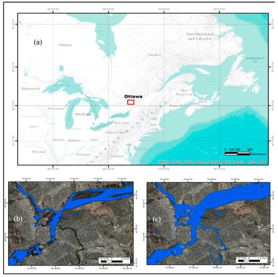
Figure 1.
(a) Location of study area in the North America map, (b) Ottawa and Gatineau River extents before flood (9 May 2018), (c) Flood extent on the Ottawa and Gatineau Rivers in Ottawa, Canada (10 May 2018), recorded by the International Charter: Space and Major Disasters. Flood and river extents are produced by Natural Resources Canada (NRC) based on RadarSat-2 data.

Table 1.
International Charter Space and Major Disasters activation for Ottawa flood event.
Generally, in water cycle and flood processes, the definition of watershed boundaries is very important, allowing for the delineation of land areas that catch precipitation and then drain into a water body [14]. For this purpose, we need to delineate the watershed that causes floods in Ottawa city.
According to the NRC service, Ottawa city is affected by two principal rivers: Ottawa and Gatineau, which are drained by three sub-basins: the upper, central and lower Ottawa watershed boundaries [15].
According to the availability of discharge ground stations, we selected the Britannia station (02KF005), located at latitude 44°81′–48°68′N and longitude 76°67′–81°53′W, and recorded only the flow drained by the upper and central Ottawa watersheds (Figure 2).
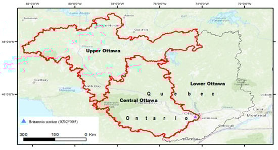
Figure 2.
Selected study area: upper and central Ottawa watersheds.
2.2. Data
Accurate flood forecasting results are related to the quality of the data which are required for two parts of the proposed methodology, i.e., hydrological discharge estimation and flood extent mapping.
For hydrological forecasting, the MILc model requires three weather related data: precipitation, air temperature and observed discharge data. For flood extent mapping, the HEC-RAS model requires geometric and flow data.
2.2.1. Precipitation Data
Precise measurements of precipitation are difficult over large areas with ground precipitation gauges. Satellite precipitation measurement from space can cover large areas by providing more frequent products around the world. Satellites carry instruments designed to observe H2O content in the atmosphere [16].
In this study, precipitation data are retrieved from SSPs in NRT. Two of NASA’s SPPs are selected with different spatial and temporal resolutions: IMERG and TMPA products (Figure 3).
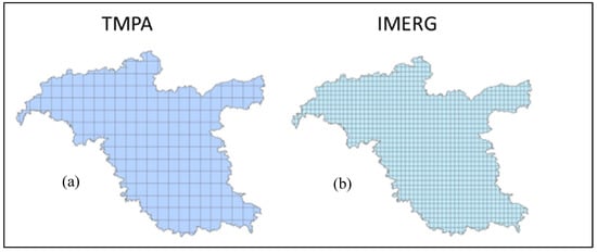
Figure 3.
Spatial resolution and footprint comparison between two satellite precipitation products: (a) tropical rainfall measurement mission multi-satellite precipitation analysis (TMPA) (0.25°) and (b) integrated multi-satellite retrievals for global precipitation measurement (IMERG) (0.1°).
Many SPPs were employed for discharge estimation purpose [17,18] such as TMPA, climate prediction center morphing technique (CMORPH) and precipitation estimation from remotely sensed information using artificial neural networks (PERSIANN). IMERG products are newly available and might offer better accuracy on flood discharge estimation and mapping.
TMPA and IMERG products are provided by a different generation of instruments. TMPA products are retrieved from a tropical rainfall measurement mission microwave imager (TMI) that covers the 10.6 GHz to 85.5 GHz frequency channels. However, IMERG products are carried out from the global precipitation measurement microwave imager (GMI) designed to observe the total precipitation within all cloud layers [19], covering larger parts of frequency channels (Table 2).
Table 2.
Metadata of satellite precipitation products. GMI = global precipitation measurement microwave imager. TMI = tropical rainfall measurement mission microwave imager.
IMERG data records (1488) and TMPA data records (248) for the period from 10 April 2017 to 10 May 2017 were acquired from GIOVANNI, a NASA Earth data platform in network common data form (NetCDF).
2.2.2. Air Temperature Data
Air temperature data were collected by the ground stations located in the study area. They are also available in the NRC platform in real time [20] for the same period from 10 April 2017 to 10 May 2017.
2.2.3. Observed Discharge Data
Discharge and water depth data were observed by Britannia (02KF005) ground stations, located downstream of the Ottawa River watershed. Regularly, the base flow in this station is about 2800 m3/s, while discharge can reach 5400 m3/s (Figure 4). The observed discharge data are very important in this study because they are used for estimating the MILc model parameters and validating the forecasted flood discharge by SPPs. The data are available at the NRC platform in real time for the same period from 10 April 2017 to 10 May 2017.
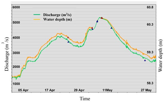
Figure 4.
Discharge hydrograph observed by the Britannia (02KF005) ground station from 01 April 2017 to 31 May 2017 located downstream of the Ottawa River. The red triangles represent control measurements of water depth, and the blue triangles represent control measurements of discharge.
2.2.4. Geometric Data
Geometric data are used to build models of terrain neighboring the rivers and the area desired for flood mapping. The accuracy of geometric data is very important because the terrain governs the movement of precipitation when it reaches the ground. The HEC-RAS model allows the use of DEM. In this study, we selected open source shuttle radar topography mission (SRTM) DEM [21] with 1 arc-second of spatial resolution for the modeling process.
2.2.5. Flow Data
According to the goal of the methodology, two input hydrographs are processed: the forecasted discharge from SPPs, specifically IMERG, and the observed discharge by a ground station located downstream of the Ottawa River in order to compare the accuracy and the impact of discharge data in flood extent mapping.
3. Methodology
The early warning in flood disaster management has grown with the availability of real time data. The most crucial part of a flood forecasting system is the hydrological model. Many categories of flood forecasting methods exist [22] with same expectations, namely the discharge hydrograph estimation, the volume of water in the stream, however, the difference concerns the modelling approach, the number of parameters and the type of used data. In our work, the R–R model based on SPPs in NRT was selected. Our approach was divided into two parts: hydrological forecasting in NRT and flood extent mapping in NRT.
The new global flood forecasting framework is described in Figure 5:
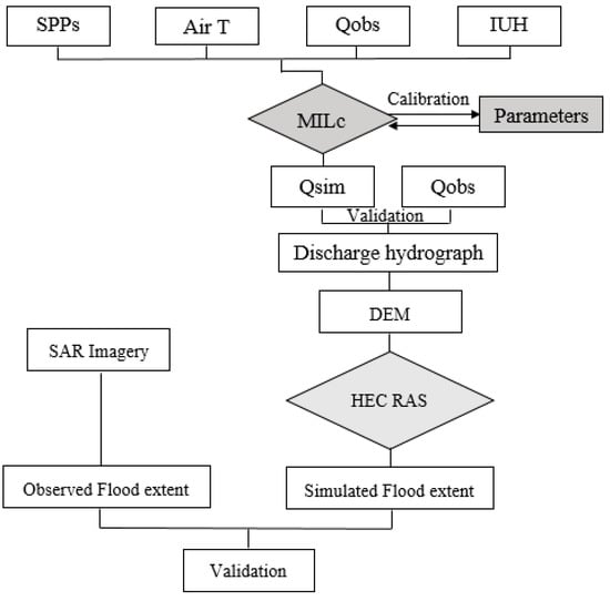
Figure 5.
Hydrological flood forecasting framework based on the MILc model and SPPs. MILc = Continuous Lumped Hydrological Model; SPPs = satellite precipitation products; Air T = air temperature; IUH = instantaneous unit hydrograph; Qobs = observed discharge and Qsim = simulated discharge. Flood extent mapping based on the Hydrological Engineering Center River Analysis System (HEC-RAS) model and forecasted discharge hydrographs from SSPs and RadarSat-2 imagery during the flood event is used for accuracy assessment and validation of the framework.
3.1. Hydrological Forecasting in NTR
Hydrological forecasting aims to predict a flood discharge hydrograph based on SPPs. For this purpose, we selected an open source hydrological model which allows the use of SPPs. Kauffeldt et al. provide a comprehensive review of flood forecasting systems [22], which permits an appropriate model selection. We chose the MILc R–R model developed by Brocca et al. [9]. This model only applies for gauged watersheds, offering the possibility to validate expected results.
3.1.1. MILc Model
MILc consists of the soil–water balance model (SWB) and the rainfall–runoff model (R–R) that are used to simulate temporal soil moisture patterns and flood discharge, respectively. The two models have a linear relationship. It has been confirmed by [17] that an accurate estimation of the antecedent wetness condition (AWC) on the hydrologic response of a watershed can provide a better accuracy for the flood hydrograph. The MILc model has been tested for flood simulation based on rain ground station data [9,10]. In this paper, we developed an independent function to adapt the MILc model to use SPPs.
The surface soil layer is assumed as a spatially lumped system, which can be expressed in the following water content balance equation:
where t is time, W(t) is the amount of water in the soil layer, f(t) is the fraction of the precipitation infiltrating into the soil, e(t) is the evapotranspiration rate, g(t) is the drainage rate due to the interflow and/or the deep percolation and Wmax is the maximum water capacity of the soil layer. The ratio W(t)/Wmax represents the degree of saturation.
The R–R model is based on the soil conservation service curve number method [23] aimed to estimate the direct runoff from precipitation excess for each sub-watershed. The respective sub-watershed drains water into the principal stream. Finally, the routing along the principal stream is estimated by the diffusive linear method.
Therefore, the precipitation excess, εj(t) for the element j (j D 1, …, Nb) is given by the soil conservation service curve number formulation [24]:
where Rj(t) is the precipitation depth from the start of the rainstorm, Sj is the soil potential maximum retention at the start of the rainstorm, D is the diffusivity parameter and λ1 is the parameter linked to the initial abstraction and assumed constant for all elements.
3.1.2. Model Adaptation to SPPs
In order to integrate SPPs with the MILc model, we developed an independent function for areal precipitation extraction, which allows us to use the global coverage SPPs in the MILc model for flood forecasting. Although many methods exist for this purpose, we selected the Thiessen polygon method [25], which assumes that the precipitation value at a given area (A) is covered by a pixel (i). So, the precipitation value observed at pixel i is related only to its area. The weight of every pixel is determined by the corresponding area in the Thiessen polygon network. The Thiessen polygon equation is:
So:
The following framework (Figure 6) illustrates the adaption of the MILc model for SPPs.
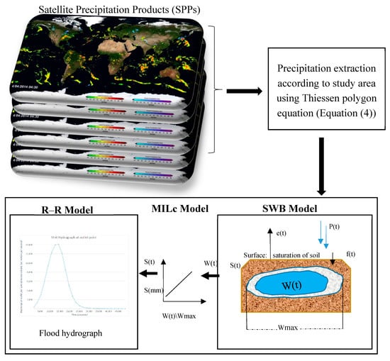
Figure 6.
Hydrological forecasting framework using the MILc model adapted to SPPs. Notations in the Soil–Water Balance model (SWB): e(t) = evapotranspiration, f(t) = infiltration, s(t) = saturation excess, p(t) = precipitation, w(t) = wetness and wmax = maximum wetness.
3.1.3. Model Performance
For MILc model performance assessment, we selected the most widely used statistics on hydrological modeling, the Nash–Sutcliffe Efficiency (NSE) and the Adapted Nash–Sutcliffe Efficiency (ANSE), proposed by Nash and Sutcliffe [26]. The ANSE, which is adapted to high flow conditions, is considered be more significant than NSE because the Ottawa River is characterized by high flow. NSE and ANSE ranges are between −∞ and 1. The United States Geological Survey (USGS, Reston, VA, USA) considers that the results are satisfactory when the NSE and ANSE values are higher than 0.5 and close to 1.
The following are the equations of NSE and ANSE:
and
where Qobs is observed discharge and Qsim is simulated discharge
3.2. Flood Mapping in NTR
The second part of the methodology aims to simulate a flood extent map using a two-dimensional (2D) flood model. For this, we propose a simple flood mapping approach in order to simulate flood extent based on open source data and software that would be compared with the observed benchmark flood extent. The HEC-RAS model requires geometric data that will be derived from DEM and discharge hydrograph data. Two discharge data were tested in different simulations and compared: (1) the forecasted discharge estimated by SPPs and (2) the observed discharge data by the ground station. Finally, to validate the simulated flood extent maps, we extracted the flood extent from the SAR imagery acquired during the flood event by RadarSat-2. The observed and simulated maps were compared using across topographical profiles for the accuracy assessment.
3.3. Flood Mapping Assessment
Based on the across topographical profiles, we estimated the distance in meters of boundaries between the simulated flood extent based on the forecasted discharge hydrograph using IMERG and the MILc model (S IMERG), and the simulated flood extent based on the observed discharge hydrograph using the ground station (S GDS) with the observed benchmark of the Ottawa River flood by RadarSat-2 (Obs).
Two methods are used to calculate the uncertainties. The first one is the absolute error (A Err), which is the difference between the simulated map data and the observed map data as shown in the following equation:
The second one (P Err) is used to calculate the error considering the pixel size (90 m) of the 2D mesh used in the HEC-RAS model for flood map simulations, based on the following equation:
3.4. Model Calibration
Calibration aims to adapt the model for the study area characteristics. The model parameters are physically based and estimated by the MILc model using the Ottawa River watershed data. Nine parameters have been estimated. These parameters and their ranges are shown in Table 3.
Table 3.
MILc model parameters.
4. Results and Discussion
4.1. Hydrological Forecasting in NRT
Accuracy Assessment
Before the calibration of the MILc model, both SPP results show high error values. With IMERG as input, values of NSE and ANSE are equal to −23.0073 and −21.7878, respectively, which reflects the significant difference between the modeled discharge and the observed discharge from the ground station.
Simulation accuracies after MILc model calibration with the data during the flood event of the Ottawa River watershed improved a lot, as shown in Table 4 by NSE and ANSE values. For the IMERG product, the model was able to accurately reproduce the observed discharge (Figure 7a), especially in high flow conditions. This is a very valuable finding and could be useful for flood forecasting for poorly or totally ungauged watersheds with high and low flow conditions. The difference between the observed and modeled discharge is small, with NSE and ANSE equal to 0.8039 and 0.8287, respectively. However, for the TMPA product, the results show that the comparison between the observed and modeled discharge is not close to the 0.5 nominal value (Table 4). The simulated discharge hydrograph by TMPA does not reproduce the shape of the observed hydrograph (Figure 7b). The IMERG product gives better results compared to TMPA in discharge estimation. According to these results, we selected the IMERG product as the input for flood extent mapping.
Table 4.
Comparison between integrated multi-satellite retrievals for global precipitation measurement (IMERG) and tropical multi-satellite precipitation analysis (TMPA) performance on discharge estimation.
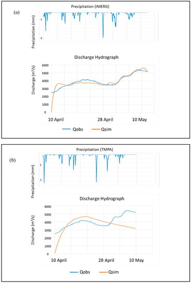
Figure 7.
Comparison between the observed (Qobs) and the simulated (Qsim) discharge obtained by the MILc model based on satellite precipitation products after calibration for (a) IMERG and (b) TMPA precipitation data.
4.2. Flood Mapping in NRT
For flood extent mapping, two accurate simulations were completed: flood extent estimated by the MILc model using SPPs (specifically IMERG) and flood extent estimated by using observed discharge from the ground station. Floods typically occur in a short time. So, it is very difficult to assess the accuracy of the simulated flood extent map without the observed flood benchmark acquired during the flood event. In this research, RadarSat-2 imagery acquired on 09 May 2017 during the Ottawa flood event was used as benchmark. By overlaying the flood extent maps, we can compare the simulated results.
It can be seen that the agreement between the simulated maps of flood extent based on IMERG and the MILc model and the retrieved maps from RadarSat-2 are reasonable (Figure 8). The global shape of the simulated flood extent generally fits well with the observed, as shown in Figure 8a for upstream and Figure 8b for the middle of the Ottawa River. For downstream, the difference between the simulated maps and the retrieved (Figure 8c) is generally small, except in locations where the water was separated from the main river channel. These uncertainties were mainly due to the used thresholding method which separated different intensity values in the histogram according to different backscattering from objects (smooth from rough surfaces) in SAR imagery. Consequently, it is difficult to separate water bodies from other land cover types when they were mixed together. For example, in Figure 8c, it can be seen that the water bodies are mixed with the urban area.
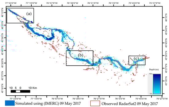
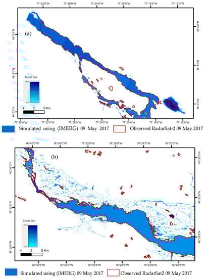
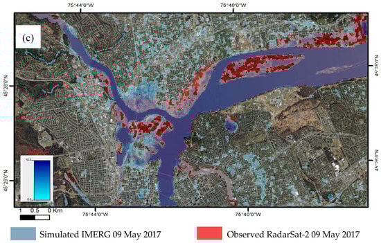
Figure 8.
Accuracy assessment between the simulated maps and the observed flood extent. (a), (b) and (c) are zooms showing upstream, middle and downstream of the Ottawa River, respectively.
To quantify the accuracy of the results, we compared across topographical profiles of flood simulated maps based on forecasted discharge hydrographs using SPPs and the MILc model with those based on the observed discharge hydrograph using the ground station. These two maps were also compared with the observed flood benchmark of the Ottawa River by RadarSat-2 (Figure 9). Ten topographical profiles were created from upstream of the Ottawa River to downstream with an equal distance of 25 km, as shown in Figure 9a. Overlaying of simulation flood extents with the observed flood extent by RadarSat-2 for two profiles, 2 and 8, is shown in Figure 9b,c, respectively, which shows the close agreement between the simulations and the observations.
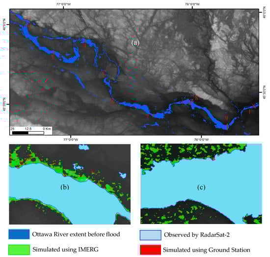
Figure 9.
(a) Locations of topographical profiles in the study area. (b,c) Overlaying of simulation flood extents with the observed flood extent by RadarSat-2 during the Ottawa flood event.
Each profile was created based on flood extent maps simulated using IMERG products and observed by RadarSat-2. With these profiles, absolute error (Equation (7)) and pixel error (Equation (8)) can be calculated, e.g., Profile 4 as shown in Figure 10.
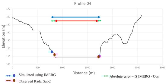
Figure 10.
Accuracy assessment of the simulated flood map using topographical profile across the Ottawa River. S IMERG = simulated IMERG.
For both sides of the riverbank, eight profiles out of ten show that the difference between the simulation map based on IMERG and the MILc model with simulation map based on observations from ground stations is equal to zero, except on the right side of Profile 3 and the left side of Profile 6. P Err values are reasonable (Table 5) considering that the pixel size of the 2D mesh used on the simulation is 90 m, except for the right side of Profile 3 and Profile 9. The use of discharge flood hydrographs based on IMERG and the MILc model for flood forecasting and mapping gives a satisfactory accuracy.
Table 5.
Accuracy assessment of simulation flood maps.
5. Conclusions
It can be concluded from this paper that the estimation of discharge flood hydrographs based on IMERG products gives satisfactory accuracy. Consequently, flood forecasting based on IMERG products can play an important role in preparedness and mitigation of flood disaster management. The IMERG products might contribute to the use of space technologies more efficiently in flood risk reduction in emergency responses on global scale due to its large coverage.
The use of forecasted flood discharge hydrographs based on IMERG and the MILc model gives encouraging results on flood extent mapping. These results were evaluated and compared with simulated flood extent maps based on observed discharge hydrographs by using ground stations. The difference between the two simulations is insignificant. The two simulations were evaluated, and the results were satisfactory with the observed flood benchmark by RadarSat-2 imagery during the flood event. The use of SAR imagery as a benchmark was helpful in accuracy assessment, due to the difficulty of acquisition of benchmark data for natural phenomenon that can happen in a short time.
Author Contributions
N.B. and F.Z. and Y.T. conceived and designed the experiments; N.B. performed the experiments; N.B. and F.Z. analyzed the data; N.B. and F.Z. and L.B. contributed to materials/analysis tools; N.B. and F.Z. and Y.H. wrote the paper.”
Funding
This work was supported by the Chinese Natural Science Foundation (Project 41771382).
Acknowledgments
The authors are thankful to the anonymous reviewers who provided constructive comments to improve this manuscript.
Conflicts of Interest
The authors declare no conflict of interest.
Acronyms
| NRT | Near-real-time |
| SPPs | Satellite precipitation products |
| MILc | Modello Idrologico lumped in continuo |
| IMERG | Integrated multi-satellite retrievals for global precipitation measurement |
| TMPA | Tropical rainfall measurement mission multi-satellite precipitation analysis |
| NSE | Nash–Sutcliffe efficiency |
| ANSE | Adapted Nash–Sutcliffe efficiency |
| SAR | Synthetic aperture radar |
| IRPI | Istituto di Ricerca per la Protezione Idrogeologica |
| R–R | Rainfall–runoff |
| DEM | Digital elevation model |
| HEC-RAS | Hydrological Engineering Center River Analysis System |
| NRC | Natural Resources Canada |
| CMORPH | CPC MORPHing technique |
| PERSIANN | Precipitation estimation from remotely sensed information using artificial neural networks |
| TMI | Tropical rainfall measurement mission microwave imager |
| GMI | Global precipitation measurement microwave imager |
| NetCDF | Network common data form |
| SRTM | Shuttle radar topography mission |
| IUH | Instantaneous unit hydrograph |
| SWB | Soil–water balance |
| AWC | Antecedent wetness condition |
| USGS | United States Geological Survey |
References
- Teng, J.; Jakeman, A.J.; Vaze, J.; Croke, B.F.; Dutta, D.; Kim, S. Flood inundation modelling: A review of methods, recent advances and uncertainty analysis. Environ. Model. Softw. 2017, 90, 201–216. [Google Scholar] [CrossRef]
- Tarpanelli, A.; Amarnath, G.; Brocca, L.; Massari, C.; Moramarco, T. Discharge estimation and forecasting by MODIS and altimetry data in Niger-Benue River. Remote Sens. Environ. 2017, 195, 96–106. [Google Scholar] [CrossRef]
- United Nations Office for Disaster Risk Reduction (UNISDR). Centre for Research on the Epidemiology of Disasters (CRED). The Human Cost of Weather-Related Disasters 1995–2015. Available online: http://www.unisdr.org/2015/docs/climatechange/COP21 Weather Disasters Report 2015 FINAL.pdf (accessed on 9 March 2018).
- Kwak, Y.; Arifuzzanman, B.; Iwami, Y. Prompt proxy mapping of flood damaged rice fields using MODIS-derived indices. Remote Sens. 2015, 7, 15969–15988. [Google Scholar] [CrossRef]
- Revilla-Romero, B.; Hirpa, F.A.; Pozo, J.T.D.; Salamon, P.; Brakenridge, R.; Pappenberger, F.; de Groeve, T. On the use of global flood forecasts and satellite-derived inundation maps for flood monitoring in data-sparse regions. Remote Sens. 2015, 7, 15702–15728. [Google Scholar] [CrossRef]
- Giustarini, L.; Hostache, R.; Matgen, P. A change detection approach to flood mapping in urban areas using TerraSAR-X. IEEE Trans. Geosci. Remote Sens. 2013, 51, 2417–2430. [Google Scholar] [CrossRef]
- Shrestha, R.; Di, L.; Eugene, G.Y.; Kang, L.; Shao, Y.Z.; Bai, Y.Q. Regression model to estimate flood impact on corn yield using MODIS NDVI and USDA cropland data layer. J. Integr. Agric. 2017, 16, 398–407. [Google Scholar] [CrossRef]
- World Meteorological Organization (WMO). Manual on Flood Forecasting and Warning. Available online: http://www.wmo.int/pages/prog/hwrp/.../flood_forecasting_warning/WMO%201072_en.pdf (accessed on 1 March 2018).
- Moradkhani, H.; Sorooshian, S. General review of rainfall-runoff modeling: Model calibration, data assimilation, and uncertainty analysis. In Hydrological Modelling and the Water Cycle; Springer: Berlin, Germany, 2009; pp. 1–24. [Google Scholar]
- Brocca, L.; Melone, F.; Moramarco, T. Distributed rainfall-runoff modelling for flood frequency estimation and flood forecasting. Hydrol. Process. 2011, 25, 2801–2813. [Google Scholar] [CrossRef]
- Brocca, L.; Liersch, S.; Melone, F.; Moramarco, T.; Volk, M. Application of a model-based rainfall-runoff database as efficient tool for flood risk management. Hydrol. Earth Syst. Sci. 2013, 17, 3159. [Google Scholar] [CrossRef]
- US Army Corps of Engineering. Hydrologic Engineering Center. 2D Modeling User’s Manual; US Army Corps of Engineering: Washington, DC, USA, 2016; Volume 5.
- International Charter: Space & Major Disasters. Flood Event in Canada. Available online: https://disasterscharter.org/web/guest/-/flood-in-canada-call-608 (accessed on 5 December 2017).
- Partnerships & Strategies Section Alberta Environment. Glossary of Terms Related to Water and Watershed Management in Alberta; Partnerships & Strategies Section Alberta Environment: Alberta, AB, Canada, 2008. [Google Scholar]
- Esri Canada Education. Water Survey of Canada. Upper, Central and Lower Ottawa Watershed Boundaries. Available online: https://www.arcgis.com/home/item.html?id=12b6e33d5a754c92b97ae5d0fed6940a (accessed on 9 December 2017).
- National Aeronautics and Space Administration (NASA). Global Precipitation Measurement Core Observatory. Available online: https://pmm.nasa.gov/sites/default/files/documentfiles/GPM%20Mission %20Brochure.pdf (accessed on 14 February 2018).
- Ciabatta, L.; Brocca, L.; Massari, C.; Moramarco, T.; Gabellani, S.; Puca, S.; Wagner, W. Rainfall-runoff modelling by using SM2RAIN-derived and state-of-the-art satellite rainfall products over Italy. Int. J. Appl. Earth Obs. Geoinf. 2016, 48, 163–173. [Google Scholar] [CrossRef]
- Hong, Y.; Hsu, K.L.; Moradkhani, H.; Sorooshian, S. Uncertainty quantification of satellite precipitation estimation and Monte Carlo assessment of the error propagation into hydrologic response. Water Resour. Res. 2006, 42. [Google Scholar] [CrossRef]
- National Aeronautics and Space Administration (NASA). GPM Microwave Imager Instrument for NASA and JAXA. Available online: https://pmm.nasa.gov/GPM (accessed on 14 February 2018).
- Natural Resources of Canada (NRC). Discharge and Air Temperature Data. Available online: https://eau.ec.gc.ca/report/ real_time_f.html (accessed on 10 January 2018).
- US Geological Survey (USGS). Digital Elevation Model Data. Available online: https://earthexplorer.usgs.gov (accessed on 2 January 2018).
- Kauffeldt, A.; Wetterhall, F.; Pappenberger, F.; Salamon, P.; Thielen, J. Technical review of large-scale hydrological models for implementation in operational flood forecasting schemes on continental level. Environ. Model. Softw. 2016, 75, 68–76. [Google Scholar] [CrossRef]
- Michel, C.; Andréassian, V.; Perrin, C. Soil conservation service curve number method: How to mend a wrong soil moisture accounting procedure? Water Resour. Res. 2005, 41. [Google Scholar] [CrossRef]
- Chow, K.W.; Ko, N.W.M.; Leung, R.C.K.; Tang, S.K. Inviscid two-dimensional vortex dynamics and a soliton expansion of the sinh-Poisson equation. Phys. Fluids 1998, 5, 1111–1119. [Google Scholar] [CrossRef]
- Goovaerts, P. Geostatistical approaches for incorporating elevation into the spatial interpolation of rainfall. J. Hydrol. 2000, 228, 113–129. [Google Scholar] [CrossRef]
- Krause, P.; Boyle, D.P.; Bäse, F. Comparison of different efficiency criteria for hydrological model assessment. Adv. Geosci. 2005, 5, 89–97. [Google Scholar] [CrossRef]


© 2019 by the authors. Licensee MDPI, Basel, Switzerland. This article is an open access article distributed under the terms and conditions of the Creative Commons Attribution (CC BY) license (http://creativecommons.org/licenses/by/4.0/).