Article

Temporal Decorrelation of C-Band Backscatter Coefficient in Mediterranean Burned Areas

by
Miguel A. Belenguer-Plomer
1,*,
Emilio Chuvieco
1 and
Mihai A. Tanase
1,2
1
Environmental Remote Sensing Research Group, Dep. of Geology, Geography and Environment, Universidad de Alcalá, Colegios 2, 28801 Alcalá de Henares, Spain
2
National Institute for Research and Development in Forestry, Bulevardul Eroilor nr. 128, 077190 Voluntari, Ilfov, Romania
*
Author to whom correspondence should be addressed.
Remote Sens. 2019, 11(22), 2661; https://doi.org/10.3390/rs11222661
Submission received: 11 October 2019 / Revised: 9 November 2019 / Accepted: 11 November 2019 / Published: 14 November 2019

Abstract

:
Burned area algorithms from radar images are often based on temporal differences between pre- and post-fire backscatter values. However, such differences may occur long past the fire event, an effect known as temporal decorrelation. Improvements in radar-based burned areas monitoring depend on a better understanding of the temporal decorrelation effects as well as its sources. This paper analyses the temporal decorrelation of the Sentinel-1 C-band backscatter coefficient over burned areas in Mediterranean ecosystems. Several environmental variables influenced the radar scattering such as fire severity, post-fire vegetation recovery, water content, soil moisture, and local slope and aspect were analyzed. The ensemble learning method random forests was employed to estimate the importance of these variables to the decorrelation process by land cover classes. Temporal decorrelation was observed for over 32% of the burned pixels located within the study area. Fire severity, vegetation water content, and soil moisture were the main drivers behind temporal decorrelation processes and are of the utmost importance for areas detected as burned immediately after fire events. When burned areas were detected long after fire (decorrelated areas), due to reduced backscatter coefficient variations between pre- to post-fire acquisitions, water content (soil and vegetation) was the main driver behind the backscatter coefficient changes. Therefore, for efficient synthetic aperture radar (SAR)-based monitoring of burned areas, detection, and mapping algorithms need to account for the interaction between fire impact and soil and vegetation water content.

1. Introduction

Fire has a key role in the global climatic balance modifying the greenhouse gases (GHGs) emission fluxes and the presence of aerosols in the atmosphere [1,2,3]. The Global Climate Observing System (GCOS) considers fire disturbance as an essential climatic variable (ECV) due to the close relationship between fire regime and climate. According to Bojinski et al. [4], an ECV is a physical, chemical, biological, or a group of linked variables that have a major influence on the climate system and are key to predicting climate evolution. In 2010, the European Space Agency (ESA) started the Climate Change Initiative (CCI), a program focused on deriving remote sensing-based information on different ECVs to improve climate modeling efforts [5,6]. Given its importance for climate modeling [7,8], fire disturbance was included in the CCI program (Fire CCI) since the beginning. The aim was to produce long-term consistent time series of global burned area maps [9]. The most recent global burned area products estimate that around 4 million km 2 are burned every year [10,11]. However, there is still a remarkable uncertainty about the worldwide burned area extent [12], since the currently available global products are limited by (i) the use of passive remoted sensing datasets, which is associated with limitations in areas of persistent cloud cover (i.e., inter-equatorial latitudes), and (ii) relatively coarse spatial resolutions (250 m), which makes the detection of small fires difficult [13,14]. A recent comparison between burned area products from Sentinel-2 and Moderate Resolution Imaging Spectrometer (MODIS) for Africa indicated that the latter missed almost half of the total burned area, mostly due to small fires omission (<100 ha) [15].
Synthetic aperture radar (SAR) data have been increasingly used for land cover mapping, given their independence from cloud cover and solar illumination conditions [16,17]. Burned area mapping algorithms have been developed from diverse SAR images, such as those acquired by the European Remote Sensing (ERS) satellites (ERS-1 and ERS-2) [18,19,20,21,22,23,24], RADARSAT [17,25], and the Advanced Land Observation Satellite (ALOS) Phased Array type L-band Synthetic Aperture Radar (PALSAR) [26]. These SAR-based approaches were, however, limited by (i) the low temporal resolution of the satellites; (ii) the reduced number of polarizations available; (iii) the steep viewing geometries, which were less suitable for vegetation monitoring; and (iv) data access restrictions. With the launch of ESA’s Sentinel-1 satellites these shortcomings were largely eliminated due to the significant improvement of the revisit period (i.e., theoretical revisit period of three days for ascending and descending passes combined), availability of dual-polarization datasets (vertical–vertical, VV, and vertical–horizontal, VH polarizations), shallower incidence angle, and an open data access policy. Such advancements have generated interest in developing regional [27,28] to global [29] burned area mapping algorithms and products (i.e., FireCCIS1SA10 for the Amazon basin) based on Sentinel-1 SAR data. Most algorithms use the amount of signal returned to the sensor (backscatter coefficient) without considering the phase information (interferometry) as SAR data processing becomes more complex and the accuracy of the burned area product is not improved when compared to algorithms based on backscatter coefficient alone [30].
Burned area mapping approaches often use temporal differences between pre- and post-fire datasets [27,28,29,31,32]. Generally, over vegetated areas, the post-fire backscatter coefficient decreases when compared to unburned areas due to the reduction of the scattering elements (i.e., leaves and branches) through combustion [33,34]. However, opposite trends may be observed, particularly when rainfall occurs after a fire event, since the removal of vegetation allows for increased soil surface scattering particularly for the co-polarized waves [22,25,35]. Furthermore, changes of the backscatter coefficient in areas affected by fire may take place long past the fire event (up to several months), an effect known as temporal decorrelation [29,36]. One should notice that temporal decorrelation was observed not only over fire-disturbed areas and C-band data. Similar effects were observed for L-band data over areas affected by logging [37]. Therefore, a better understanding of the temporal decorrelation effects and its sources is needed to improve SAR-based burned area mapping algorithms. Thus, the specific objective of this study was to evaluate the influence of different environmental variables that may obscure fire combustion effect on the backscatter coefficient immediately after a fire.

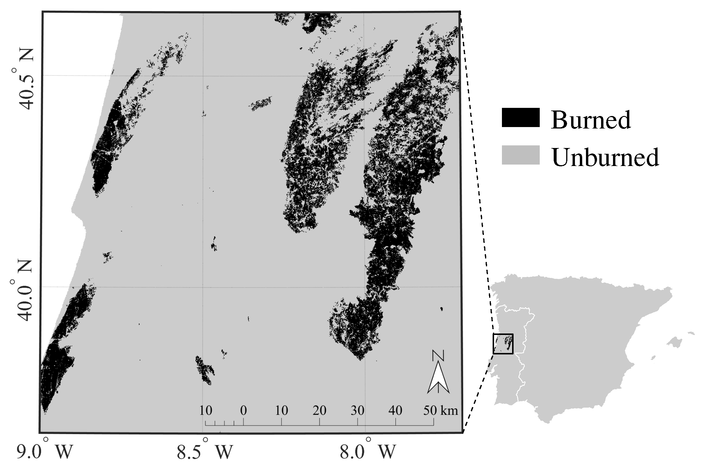
2. Study Area and Datasets

The study was carried out in Portugal over fire-affected areas located in tile 29TNE of the Military Grid Reference System (MGRS). The area was affected by large fires in 2017 (Figure 1).
Besides the large areas affected by fires, tile 29TNE was also selected since (i) Sentinel-1 A/B acquisitions from ascending and descending passes were available at the nominal temporal frequency of six days [38]; (ii) ancillary data on environmental variables at a detailed spatial resolution were available from the Copernicus Land Monitoring Service program; and (iii) cloud cover was low (annual mean cloud cover of 27.2% as computed from MODIS images) when compared to the mean cloud cover over all Europe [39], which allowed using optical sensors indices as a proxy for a range of environmental variables that informed the analysis.
The SAR dataset was formed by temporal series of dual-polarized (VV and VH polarizations) C-band backscatter coefficient acquired by the Sentinel-1 A/B sensors. The ground range detected (GRD) product acquired using the interferometric wide (IW) swath mode was downloaded from online repositories. As ancillary datasets, optical images acquired by Sentinel-2 MultiSpectral Instrument (MSI) were retrieved. The Sentinel-2 images were used to derive proxy spectral indices for a range of environmental variables (e.g., vegetation water content, fire impact) that may affect C-band scattering processes. Sentinel-1 and -2 images were retrieved from Copernicus Open Access Hub. In addition, information on land cover and surface soil moisture (SSM) were extracted from operational products available through the Copernicus Land Monitoring Service. The Corine Land Cover (CLC) 2018 Version 20b2 at 100 m pixel spacing was used to obtain information on land cover types. The Copernicus Global SSM product, derived from Sentinel-1 data, was used to obtain information on soil moisture in the top few centimetres at 1 km spacing [40]. Lastly, topographic information was derived using the global digital elevation model (DEM) available from the Shuttle Radar Topography Mission (SRTM) at 30 m pixel spacing.
Reference fire perimeters were obtained from atmospherically corrected Landsat-8 optical images retrieved from the United States Geological Survey repository (USGS). The fire perimeters were used to differentiate between burned and unburned pixels during the analysis. Landsat-8 images were used to maintain independence from the environmental variables estimated from Sentinel-2 [30].

3. Methods

3.1. Earth Observation Data

The Orfeo ToolBox (OTB), an image processing software developed by the National Centre for Space Studies (CNES) [41], was used to pre-process the Sentinel-1 GRD images. The pre-processing step includes SAR data clipping according to the specified MGRS tiles and radiometric normalization to gamma nought ( γ 0 ) through the gamma nought lookup table provided with the product metadata. The calibrated images were orthorectified to ground geometry using the topographic information derived from the SRTM. Subsequently, the orthorectified images acquired from the same orbital path, but provided within different slices, were mosaicked. Finally, a multi-temporal filtering was carried out using images from the same orbital path [42]. The GRD data were processed to 20 m (Sentinel-1 nominal spatial resolution) and aggregated in post-processing to 40 m spacing, deemed more suitable for burned area detection and mapping from the Sentinel-1 C-band backscatter coefficient due to the reduced speckle [43]. The equivalent number of looks for the temporally filtered, spatially aggregated images was on average 75.
Bottom of atmosphere (BOA) surface reflectance images were derived using the sen2cor (v.2.4.0) atmospheric correction algorithm from Level-1C (L1C) Sentinel-2 MSI images. Besides atmospheric corrections, sen2cor also allowed the ability to carry out topographic corrections based on the SRTM DEM. The resolution selected during the execution of sen2cor was 20 m, with the processed images being resampled (using a bi-cubic interpolation) to 40 m to match the spatial resolution of the processed Sentinel-1 SAR images. The soil moisture product was also resampled to 40 m using the same resampling method.

3.2. Ancillary Data

Variables that may affect the C-band scattering process from vegetated areas were evaluated to ascertain their relationship with the observed temporal decorrelation. Fire severity, vegetation growth, and vegetation water content were studied through proxies (i.e., vegetation indices) estimated from Sentinel-2 optical images. Soil surface moisture was retrieved from the Copernicus Global Land Service while the SRTM digital elevation model was used to derive the topography-related variables (i.e., local incidence angle and slope orientation).

3.2.1. Fire Severity

Fire severity is the degree of organic matter loss due to fire combustion and is strongly related to fire intensity [44]. The SAR backscatter coefficient from burned areas is conditioned by fire severity given the sensitivity to the amount of vegetation scattering elements [45,46]. To estimate fire impact on vegetation, the relativized burn ratio (RBR) proposed by Parks et al. [47] (Equation (1)) was computed. RBR was shown to accurately represent fire severity levels [48,49,50] and has a closer relationship with the composite burn index [51], in situ measurement of fire impacts on vegetation when compared to other spectral indices. The RBR was derived using the normalized burn ratio (NBR) [52] (Equation (2)) and its temporal difference between the pre- and post-fire images, the dNBR (Equation (3)).
R B R = d N B R / N B R p r e + 1.001
N B R = N I R S W I R 2 / N I R + S W I R 2
d N B R = N B R p r e f i r e N B R p o s t f i r e
where NIR and SWIR2 were derived from surface reflectivity of Sentinel-2 Bands 8A and 12, respectively.

3.2.2. Water Content

The water content of vegetation and soil may alter dielectric proprieties and hence microwaves scattering [53,54]. In this study both vegetation and soil water content were included as variables that may induce temporal decorrelation. The normalized difference water index (NDWI, Equation (4)) was shown to be related to the liquid water molecules in canopies [55] and was therefore used as a proxy to evaluate general vegetation wetness. The Copernicus Global Surface Soil Moisture product, generated at 1 km pixel spacing from Sentinel-1 data, was used as a source of soil water content information [40].
N D W I = N I R S W I R 1 / N I R + S W I R 1
where SWIR1 is the surface reflectivity of Sentinel-2 band 11.

3.2.3. Vegetation Growth
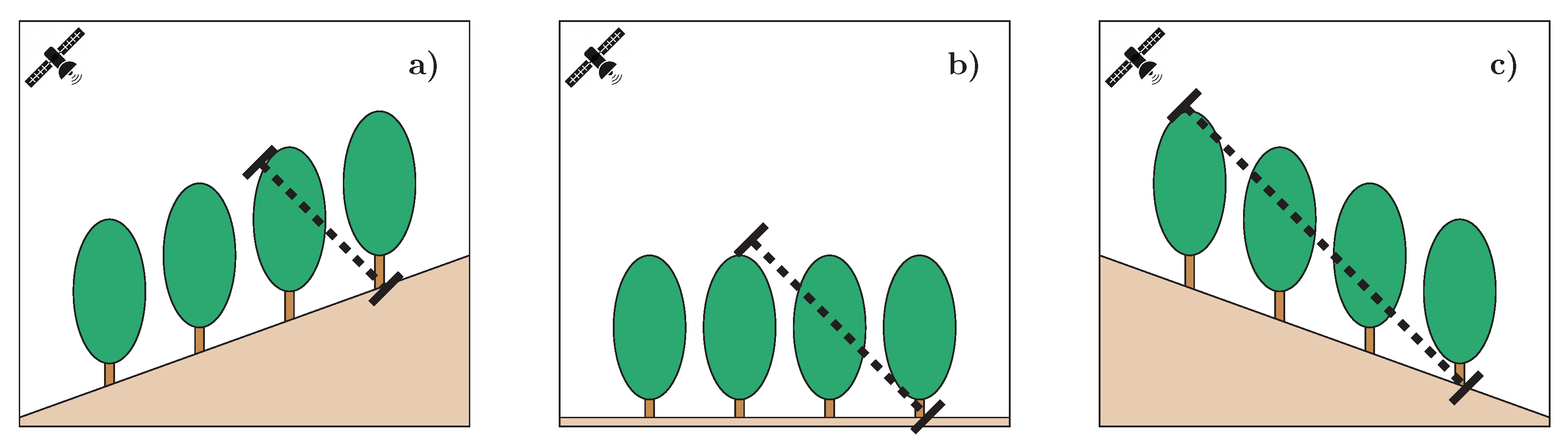
The normalized difference vegetation index (NDVI, Equation (5)) [56,57] is the most extensively used remote sensing index for vegetation monitoring [58]. This index offers information about general vegetation greenness, which depends on chlorophyll content and is related to canopy structure [59]. NDVI was used as a proxy to evaluate short-term post-fire vegetation recovery, since the saturation of the index in Mediterranean ecosystems appears between 5–10 years after the fire event, depending on the vegetation type [60,61].
N D V I = N I R R E D / N I R + R E D
where RED is the surface reflectivity of Sentinel-2 band 4.

3.2.4. Topography

Topography has a considerable influence on the C-band backscatter coefficient from burned areas through both terrain slope and its orientation with respect to the sensor looking geometry [29,62]. The local incidence angle (LIA) has been frequently used to analyze topography effects on the backscatter coefficient [25,63,64,65,66]. However, the wide swath (250 km) of the Sentinel-1 satellites (IW mode) results in an incidence angle variation of approximately 17° from near (29°) to far (46°) range. Thus, the resulting LAI values, which are conditioned by the local slope and the satellite incidence angle, may not necessarily represent the same topographic conditions from near to far range. Therefore, in this study, the local slope and the orientation angle were used to evaluate the effect of topography. Both slope and orientation (aspect) were measured in degrees and derived from the SAR looking geometry and SRTM DEM. The slope values were between 0° to 90°, meanwhile, the aspect values were between −180° and 180°. Negative values indicate slopes oriented away from the sensor while positive values indicate slopes oriented toward the sensor.

3.2.5. Land Cover

Information on land cover type was obtained from the Corine Land Cover (CLC) 2018 classification [67]. To reduce the amount of land cover classes, the CLC 2018 classification was reduced to (i) not burnable, which included artificial surfaces, water bodies, wetlands, sands, bare rocks, previous burned areas, and permanent snow and ice surfaces; (ii) crops, which included all agricultural CLC classes; (iii) herbaceous, which included the natural grasslands, sparsely vegetated areas, moors, and heathlands; (iv) shrubs, which included sclerophyllous vegetation and transitional woodland-shrub; and (v) forests, which included broad-leaved, coniferous and mixed forest CLC classes. The re-classified CLC map was resized to 40 m, through nearest-neighbor interpolation, to match the pixel spacing of the SAR images.

3.3. Reference Fire Perimeters

The reference burned perimeters were obtained following an established framework [68,69,70,71]. Landsat-8 BOA reflectance images were classified in burned, unburned, and no data (i.e., clouds, cloud shadows) using a random forests classifier trained with manually selected polygons. The polygons were digitized over a false color composite (RGB: SWIR, NIR, R) that allowed for a clear differentiation between burned and unburned patches. Polygon selection followed an iterative process (selection/ training/classification), which was repeated until the classification was deemed accurate according to a visual inspection. Finally, the reference perimeters were visually revised again to correct possible misclassifications [29]. A nearest-neighbor interpolation was utilized to resize the reference burned area perimeters to 40 m.

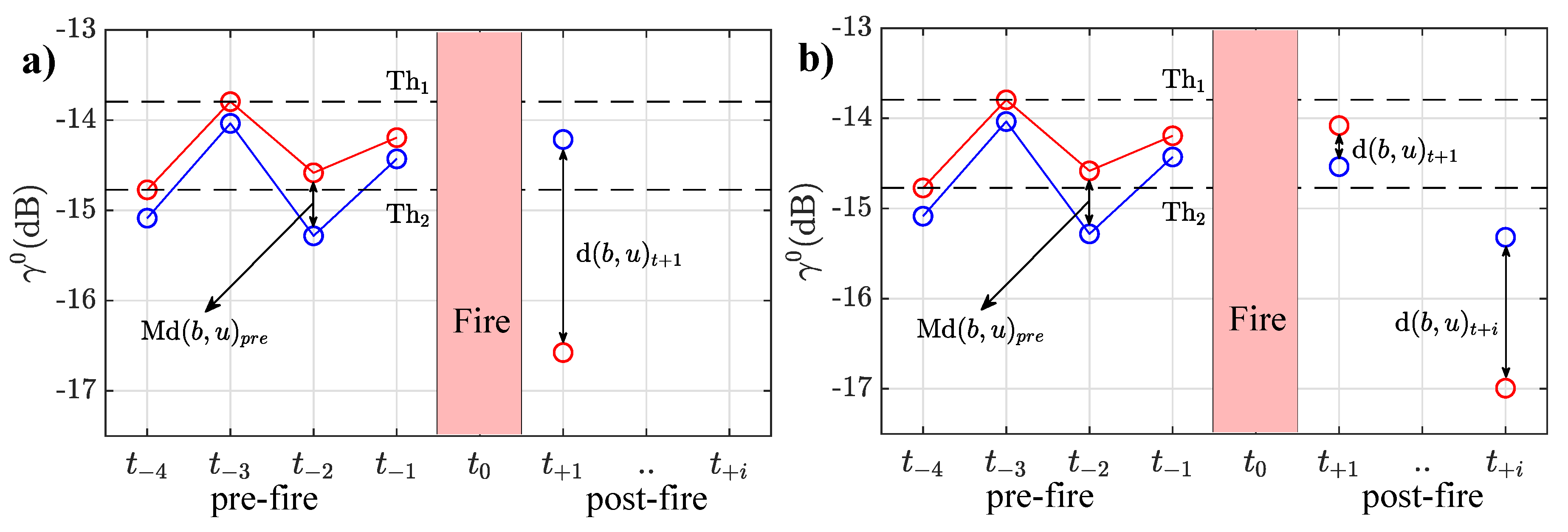
3.4. Estimating Temporal Decorrelation

In this study, only VH data were used to estimate the temporal decorrelation since the cross-polarized waves are more responsive to volumetric scattering from vegetation over Mediterranean ecosystems and less affected by changes in soil surface properties (e.g., soil moisture, surface roughness) when compared to the co-polarized (VV polarization) channel [36,72,73,74]. The different sensitivity between co- and cross-polarized waves when deriving burned area maps were previously noted by Belenguer-Plomer et al. [29].
To separate burned pixels affected by temporal decorrelation, a potential burned area detection framework was developed to determine if the temporal (pre- and post-fire) and contextual (burned and unburned) variations of VH backscatter were significant to label a pixel as burned. The potential detection framework was based on the analysis of the statistical properties of the VH backscatter coefficient (dB) within and outside the reference fire perimeters at different dates before and after the fire event date (Figure 2). The detection framework was established to ascertain the post-fire date at which a pixel may be labeled as burned using the SAR time series. The backscatter analysis was carried out for all burned pixels (determined from Landsat imagery) as well as unburned pixels located within 500 m of the fire scars. The data was first stratified by land cover class, local incidence angle [64] and slope orientation with respect to the sensor looking geometry (i.e., forward and backward-looking slopes, respectively). A pixel was labeled as burned when (i) post-fire VH backscatter was greater than the maximum or lower than the minimum backscatter values recorded for the month before the fire date ( t 0 ), and (ii) the difference between the backscatter coefficient of the pixel and the mean of the unburned reference pixels (within the corresponding land cover class) was greater than the maximum recorded during the month preceding the fire. When pre- to post-fire backscatter variations were small immediately after fire event (i.e., first post-fire SAR image, t + 1 ) but sufficiently high to label a pixel as burnt sometime after the fire and t + 1 , the pixel was considered temporally decorrelated. The lack of temporal decorrelation is exemplified in Figure 2a, as the pixel may be labeled as burned immediately after the fire ( t + 1 ). On the contrary, the presence of temporal decorrelation is shown in Figure 2b, since the pixel may be labeled as burned (according to the two criteria above) some time after the fire date and t + 1 , in t + i , being i > 1 .

3.5. Variables Analysis

The importance of the variables which affect the C-band backscattering process in burned areas (see Section 3.2) and thus on the perceived temporal decorrelation was analyzed by using an ensemble learning algorithm, the random forests [75]. Random forests is frequently used in classification problems and consists in a group of decision trees { h x , Θ z , z = 1 , } , where x is the input vector of a pixel (x), and Θ z are a sampled vectors independently bootstrapped with replacement in each decision tree (z). A unique class for x is provided from each tree, with class most often voted being finally assigned to x [75]. During the classification process, random forests computes importance measures for each independent variable [75,76]. One may use the random forest importance, whose physical meaning is based on the degree with which each variable influences the classification process [77], as information to assess the variable significance over a specific study area. Indeed, in recent years an increasing number of studies used random forests to such ends [62,78,79,80,81].
Here, the importance of the selected environmental variables was estimated by building random forest models. Such models were customized through the number of trees and training samples used. The number of trees is a key part of the random forests adjustment as it is known that the use of more trees generates a convergence of the generalization error and reduce over-fitting [75,76,82]. However, the use of more trees requires more computational resources. A preliminary empirical analysis concluded that 200 trees provided the best balance between speed and accuracy as statistically significant differences (t-test, 95% confidence interval) between variable importance scores obtained from models of 100 and 200 trees, respectively, were not observed (p-value of 0.91). The number of variables taken into account for trees growing in each split was computed as the square root of the total number of variables since this reduces the correlation of trees [76,83]. Finally, for inter-comparability purposes, the variable importance values were converted to percentages (Equation (6)) to evaluate differences between land cover classes as in previous studies [62].
% V I i k = V I i k × 100 i = 1 n V I k
where V I is the variable importance of a given variable i and a land cover class k, and n is the total number of variables considered in k.

4. Results

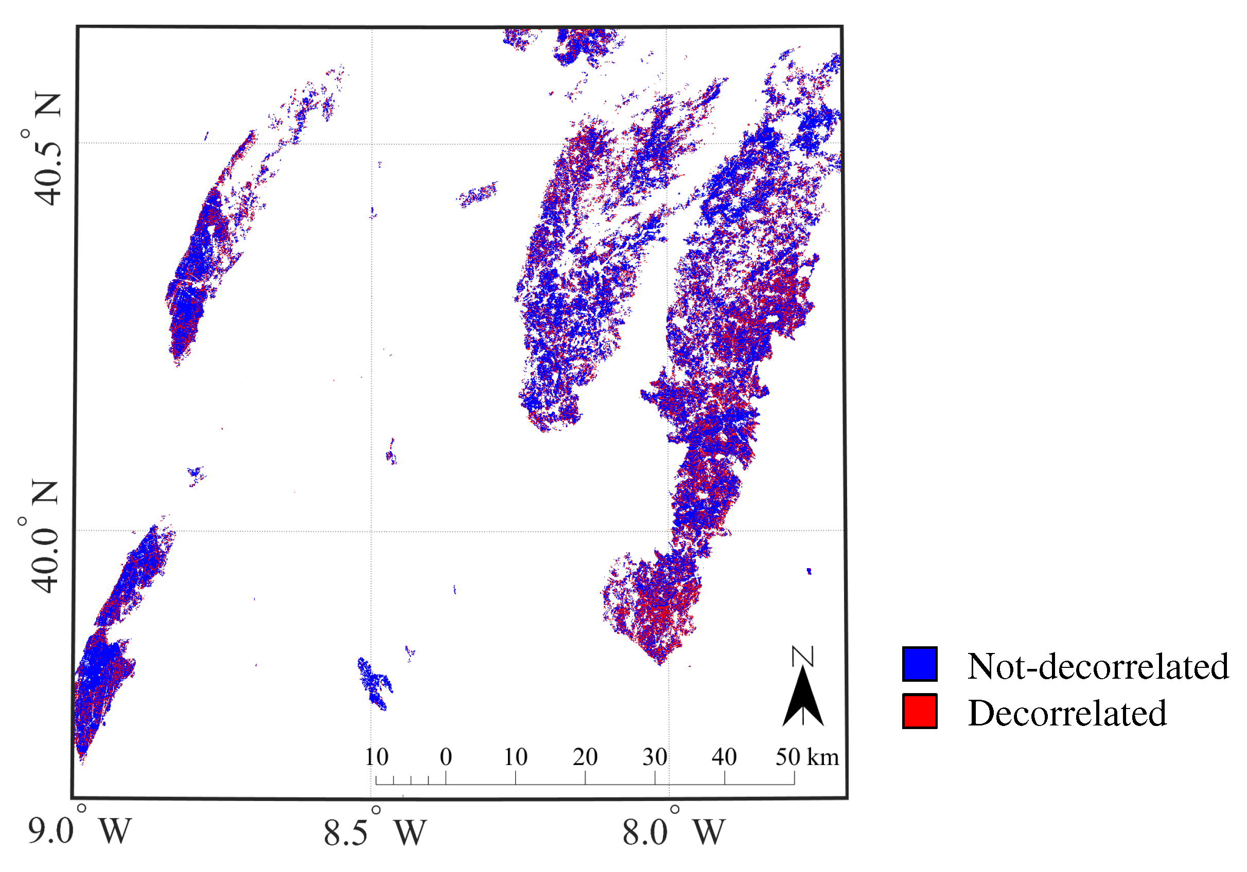
4.1. Temporal Decorrelated Pixels over Burned Areas

Over the entire study area, the frequency of pixels not affected by the temporal decorrelation (not-decorrelated pixels) was higher when compared to pixels mapped as burned at some point after the fire (Figure 3). Also, it was evident that pixels affected by temporal decorrelation were concentrated over specific areas.
Not-decorrelated pixels represented the majority (68%) of all burned pixels over all land cover classes, with decorrelated pixels representing the remaining 32% of the burned area. Over all land cover classes, most of the decorrelated pixels (86.88%) were detected within the first post-fire month (Table 1). Similar trends were observed for each land cover class. An ANOVA analysis showed no significant difference (p-value > 0.05) between the percentage of decorrelated pixels over different detection periods in each land cover class.

4.2. Decorrelation Analysis

For the first post-fire SAR acquisition, the backscatter coefficient ( γ p o s t f i r e 0 γ p r e f i r e 0 ) for not-decorrelated burned pixels decreased for all land cover classes (Figure 4, class Nd A ). Conversely, for pixels affected by temporal decorrelation, the backscatter coefficient was largely stable for the first post-fire SAR acquisition (Figure 4, class De A ). For temporally decorrelated burned pixels, the backscatter variations were considerable (Figure 4, class De B ), when considering later SAR acquisitions ( γ d e c d a t e 0 γ p r e f i r e 0 , where dec-date was the post-fire SAR acquisition when burned area detection criteria were met, see Section 3.4). However, the backscatter coefficient showed variable trends (i.e., decrease and increase) when compared to the pre-fire backscatter values.

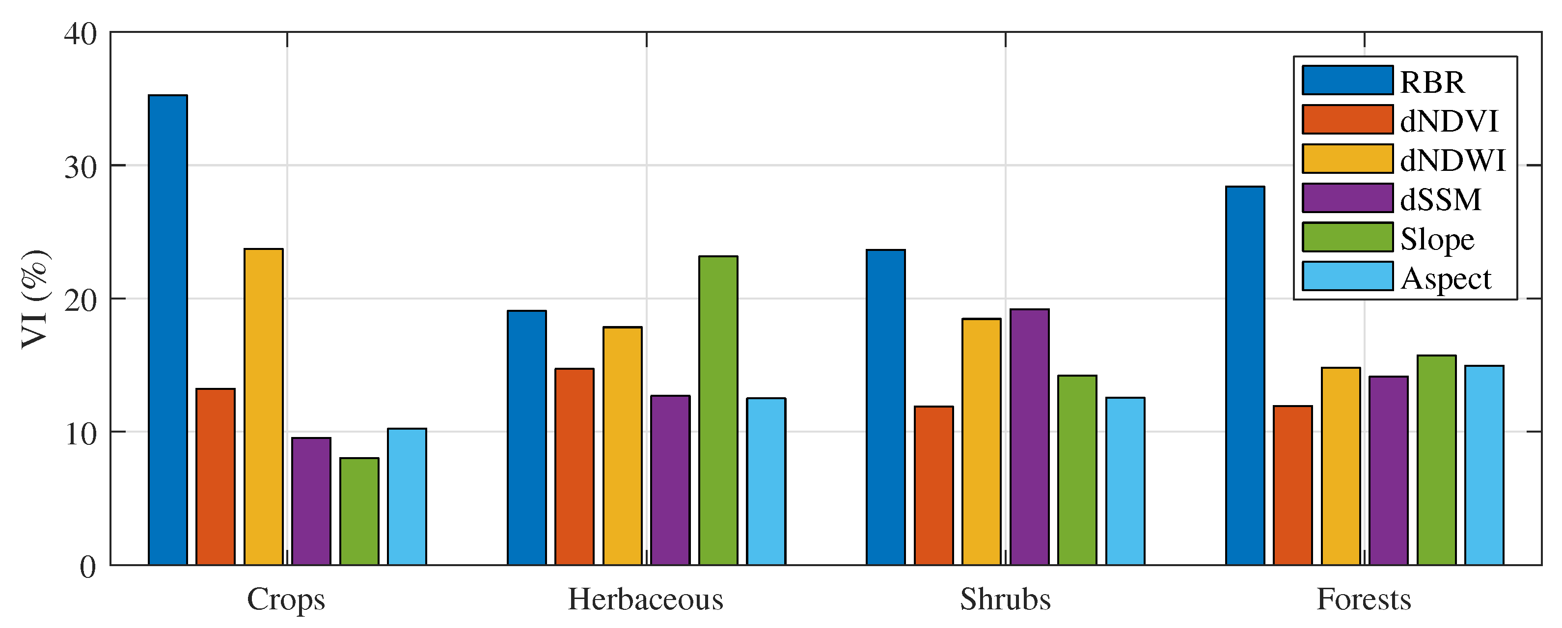
4.3. Variable Importance on Post-Fire Backscatter Coefficient

Fire severity (RBR) was evidenced as the most important variable when separating (i.e., classifying) decorrelated from not-decorrelated pixels over all land cover classes except for the Herbaceous class (Figure 5). Over Crops and Forests classes, the fire severity importance was considerably higher (around 30%) when compared to the remaining variables. For the Shrubs class, fire severity was the most important although it was closely followed by Slope and variations in the vegetation water content between post- and pre-fire images as estimated through the dNDWI. Variable importance by land cover classes was related to the mean topographic slope (Table 2). Aspect and Slope showed high importance over Herbaceous and Shrubs classes which covered higher topographic slopes when compared to the Crops and Forests classes (Table 2). The reduced importance of Aspect and Slope on the decorrelation process for the Crops class was explained by its location on low lying terrain when compared to the remaining land cover classes (Figure 6).
Histograms for post- to pre-fire backscatter coefficient change by land cover class and variable (Figure 7) show that increased fire severity translates in a high frequency of not-decorrelated pixels, except in the Herbaceous class, where no significant differences were found. The frequency of decorrelated and not-decorrelated pixels was marginally affected by changes in vegetation growth (i.e., dNDVI) and vegetation water content (i.e., dNDWI), with largely similar frequencies observed along the post-to pre-fire variables change gradient. The influence of Slope was analyzed as a function of Aspect (positive-slope oriented towards the sensor and negative-slopes oriented away from the sensor) since both variables affect the distance between canopy top and ground surface [84]. Lower distances are observed for steep slopes oriented towards the sensor when compared to flat areas and slopes oriented away from the sensor (Figure 8). Over flat areas (slope below 5°) the proportion of decorrelated and not-decorrelated pixels was similar over all land cover classes. However, over sloped areas (slopes >5°), decorrelated and not-decorrelated pixels proportions differed. For decorrelated burned pixels, post-fire soil moisture was higher when compared to not-decorrelated areas, especially when only pixels from patch size greater or equal than 1 km 2 were considered (the spatial resolution of the soil moisture product used is 1 km).

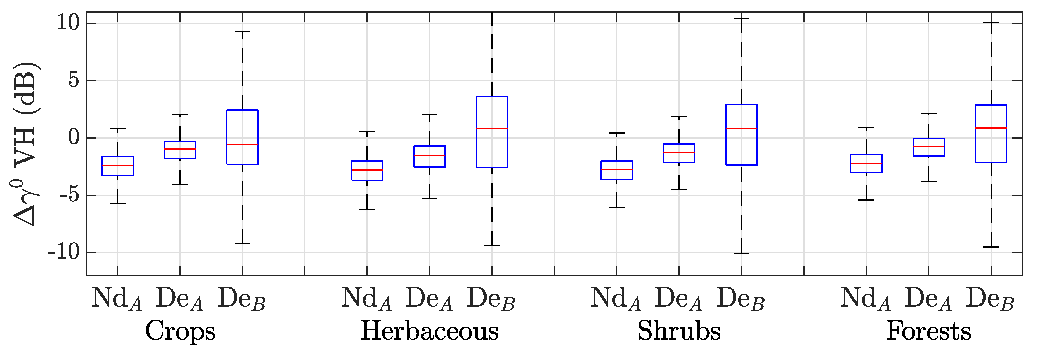
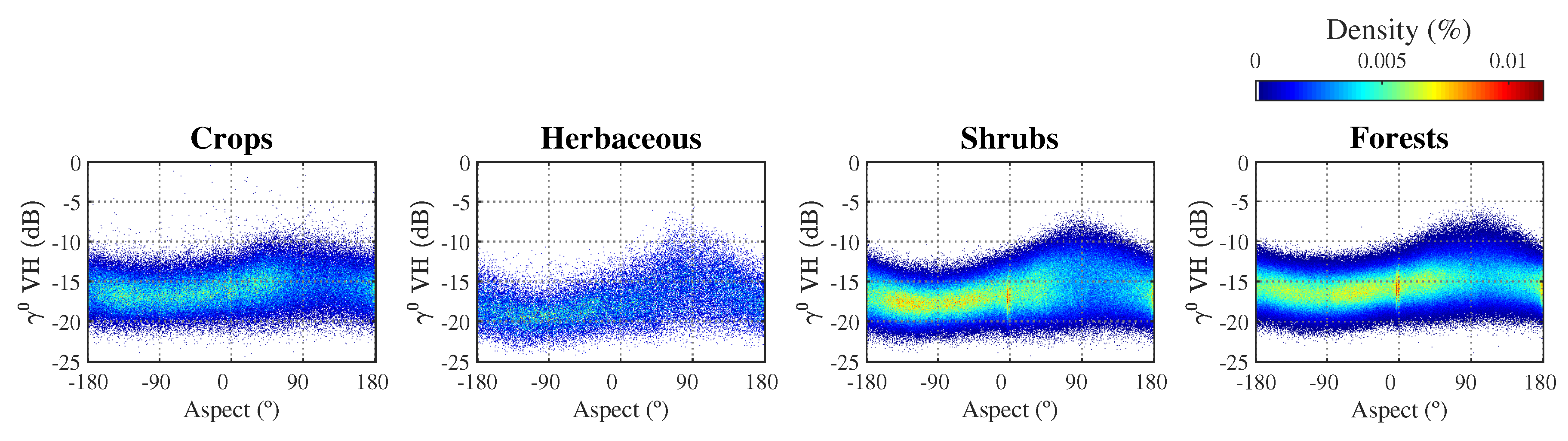
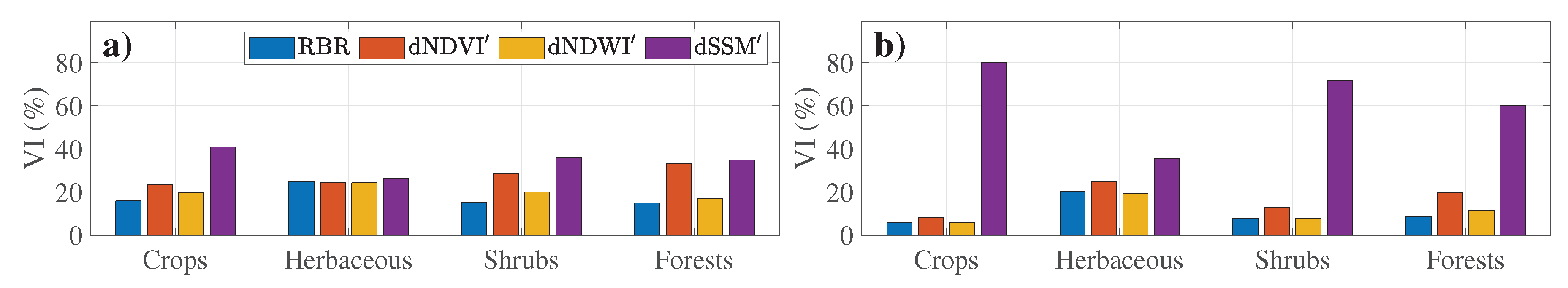
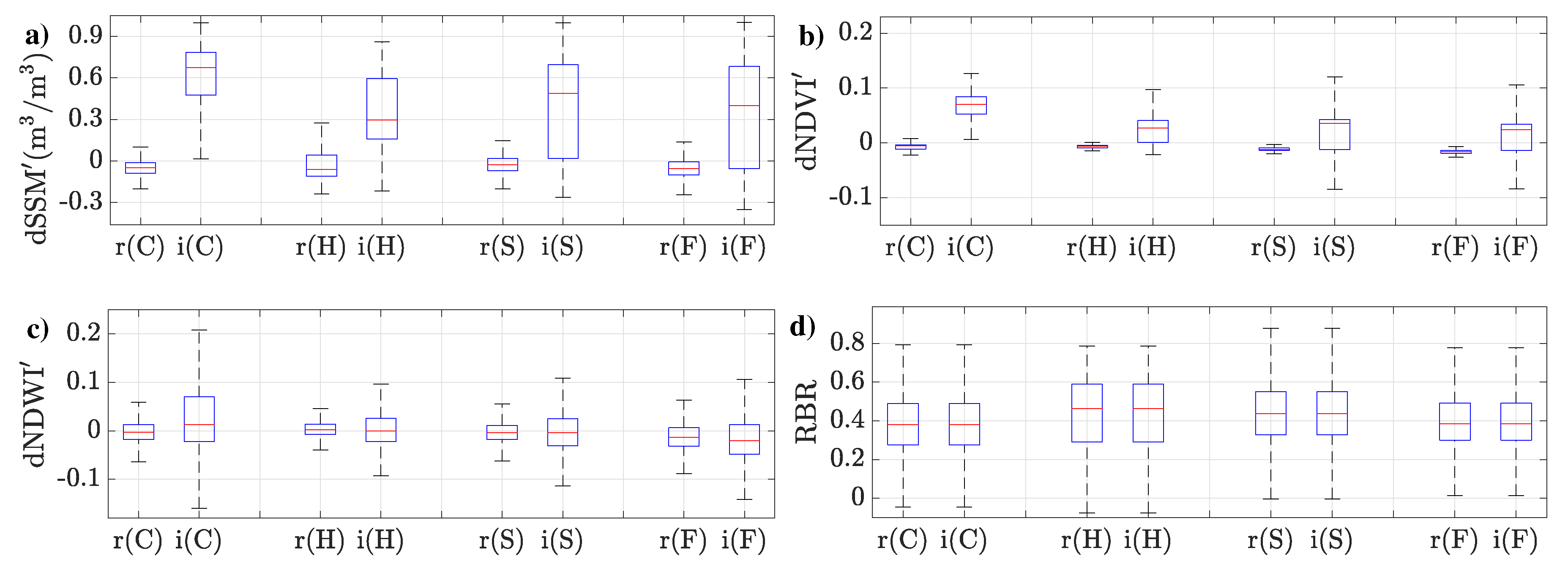
4.4. Variables Analysis over Decorrelated Pixels

As temporally decorrelated pixels are not detected immediately after the fire, it implies that some of the variables affecting the scattering process suffered variations between the post-fire date and the detection date (dec-date). The importance of each variable, except for Slope and Aspect which are not affected by temporal variations, for burned pixels detection was computed through random forests after differentiating between decorrelated pixels where the backscatter coefficient decreased (Figure 9a) and pixels where the backscatter coefficient increased (Figure 9b) with respect to the pre-fire values.
When the backscatter coefficient decreases at some point after the fire, the most important variables for burned area detection were temporal changes in soil moisture followed by vegetation growth (dSSM and dNDVI , respectively, in Figure 9a) over all land cover classes except Herbaceous for which all variables were equally important. Fire severity (RBR) importance was higher when the backscatter coefficient decreased at dec-date when compared to areas where the backscatter coefficient increased (Figure 9). Conversely, when the backscatter coefficient increased, the most important variable for burned area detection was, by a large margin, the soil moisture (dSSM in Figure 9b), although for the Herbaceous class the importance of the time differences of the soil moisture was lower when compared to the remaining land cover classes.
A backscatter coefficient reduction or increment at the dec-date, when compared to pre-fire values, for decorrelated burned pixels was mainly related to a reduction or respectively increment in soil moisture (Figure 10a). The importance of the dNDVI , particularly over Forests, when the backscatter coefficient decreased was explained by a reduction in vegetation greenness (Figure 10b,c). Decorrelated areas with backscatter decreasing between pre-fire and dec-date were affected by slightly higher fire severity when compared to areas where the backscatter increased between the two dates, particularly over the Forests class (Figure 10d).

5. Discussions

The existence of spatial patterns for decorrelated and not-decorrelated burned pixels suggested relationships between the temporal decorrelation and the environmental variables, removing the possibility that SAR speckle or detection uncertainty may induce this process randomly. Further, the radiometric uncertainty of the Sentinel-1 sensor, 0.36–0.38 dB [85], did not influence the results as most (99.7%) not-decorrelated pixels showed post- to pre-fire temporal differences above this radiometric uncertainty.
Over most land cover classes, the utmost important factor controlling the temporal decorrelation process was fire severity for which higher values were observed over not-decorrelated areas when compared to the decorrelated ones. Such a trend was explained by the higher loss of scattering elements in areas affected by high fire severity [45,46], which translates into a greater backscatter change with respect to unburned vegetation and increased the potential for detecting the affected area immediately after the fire (no temporal decorrelation). As expected, over densely vegetated areas (Forests), fire severity was the most important factor affecting the temporal decorrelation process, which aligns with previous findings related to the sensitivity of the C-band backscatter coefficient to fire impacts in the Mediterranean forests [45]. For the Herbaceous class, fire severity was the second most important factor affecting temporal decorrelation after terrain orientation with respect to the sensor looking geometry (i.e., Aspect). This may be related to the mean topographic slope of the Herbaceous class, which was higher when compared to remaining land cover classes. Besides, the divergent results of the Herbaceous may be partly explained by the reduced C-band sensitivity to fire effects over burned herbaceous or grassland areas [86] as radar waves interact more with the soil surface. For this class, Aspect had higher importance when compared to Slope as the low vegetation height and the lack of woody stems result in low C-band scattering which is further reduced after the dry season [86]. Thus, in areas covered by Herbaceous vegetation, the C-band microwaves mostly interact directly with the ground, with scattering being highly conditioned by orientation with respect to the SAR sensor (i.e., Aspect).
Water content variations had considerable importance for the decorrelation process over most land cover classes. Higher post-fire soil moisture was observed for decorrelated burned pixels when compared to not-decorrelated ones. This resulted in a higher dielectric constant and consequently a higher backscatter coefficient, which may mask out scattering decreases due to the combustion of the vegetated scattering elements since soil influence on the scattering process increases as vegetation is removed through combustion [64]. However, the perceived importance of soil moisture on the temporal decorrelation process was reduced when compared to temporal variations of vegetation water content (dNDWI) since (i) the random forests models were constructed considering all burned pixels, regardless of burned patch size. Thus, approximately half of the pixels used for training the random forests models (44.15% of decorrelated and 62.5% of not-decorrelated classes) were extracted from patches below 1 km 2 , the spacing of the soil moisture product. This may have affected the soil moisture estimation accuracy, since when only pixels from patches above 1 km 2 were analyzed, a clearer effect of soil moisture over the decorrelation process was observed; (ii) for 40% of the decorrelated pixels and 38% of the not-decorrelated ones the pre- to post-fire temporal variations in soil moisture were lower than 0.088 m 3 /m 3 , the error of the soil moisture product [40]; and (iii) the dNDWI was derived from atmospherically corrected Sentinel-2 data at the same pixel spacing as the radar images (40 m), which thus having less uncertainty when compared to the SAR based soil moisture product [87]. Sentinel-1 based soil moisture estimation may be affected by the groundwater content, intercepted rain, and SAR radiometric uncertainty [88]. These reasons may explain the difference in the observed importance on the decorrelation process between dNDWI and dSSM. However, this importance contrasts with the low differences of dNDWI between decorrelated and not-decorrelated pixels. It should be noted that random forests models allow for non-linearities and interactions between all variables considered [89]. Thus, it was evidenced that temporal decorrelation over burned areas is a complex process with several variables having a concurrent influence.
Decorrelated pixels tended to have a higher concentration over steep slopes oriented towards the sensor, especially for Herbaceous and Shrubs classes. Conversely, not-decorrelated pixels had a higher presence over shallower slopes and both, positive and negative aspects. This result supports previous findings suggesting increased C-band sensitivity to fire over sloped terrain oriented towards the radar sensor [29,64]. According to the soil moisture product, over sloped areas (>10°) soil moisture increased on average for the post-fire images in both Shrubs and Herbaceous classes. As explained above, soil moisture increment may have masked backscatter coefficient changes due to vegetation removal and consequently influenced the decorrelation process. Furthermore, the vegetation effect on the backscatter coefficient over steep slopes oriented towards the sensor (i.e., where the presence of decorrelated pixels was high) is reduced while the ground effects increased since the distance between canopy top and the ground surface is lower when compared to flat areas and slopes oriented away from the sensor [84]. Such topographic effects are reduced over Forests due to denser canopy, which reduces ground interaction of C-band microwaves and over Crops due to its predominant location over flat areas. The larger scattering elements found in Forest and Shrubs vegetation coupled with the reduced slope allowed for increased C-band scattering from vegetation. Conversely, scattering from ground was reduced, which in turn reduced the importance of the Aspect in Forest and Shrubs classes. The root mean square error of the STRM product over Portugal was estimated as 4 to 6 meters depending on land cover and terrain slope [90]. However, SRTM errors may have not affected the results of this study as most elevation errors were found over (i) abrupt slopes, covered by unburnable land cover classes; and (ii) forested areas, mainly located over flat areas and smooth slopes, with low topography related effects on radar scattering.
Over the not-decorrelated burned pixels the backscatter coefficient decreased after the fire in all land cover classes due to the reduction of vegetation scattering elements through fire-combustion, an effect particularly important for the cross-polarized waves [72,73,74]. However, over the decorrelated burned pixels both reductions and increments of the backscatter coefficient were observed, which indicates that at dec-date, a much wider range of environmental changes generated the backscatter coefficient variations needed to detect the burned area.
Backscatter coefficient reduction at dec-date, when compared to previous records, was mainly attributed to reduced soil moisture since burned areas have reduced albedo as well as increased sun exposure as a result of biomass loss. These effects may generate a higher temperature regime after the fire event, which may increase soil moisture loss [91] and result in reduced dielectric constant and consequently reduced radar scattering from the ground. Also, the vegetation combustion, which is related to the fire severity, results in a reduced number of scattering elements, which enhances the importance of soil surface scattering (and thus soil moisture) when compared to unburned areas [64,66]. Alternatively, decreasing water content and vegetation greenness after the fire may occur when trees are damaged by fire but not completely burned. Such trees maintain some scattering elements (e.g., leaves) immediately after the fire, thus sustaining higher levels of radar scattering. However, as a consequence of fire damage, such trees may not recover and die shortly after the fire, which results in reduced backscatter coefficient as dry vegetation has a lower dielectric constant when compared to healthy vegetation [92].
On the other hand, the backscatter coefficient increment at dec-date was mainly related to increased soil moisture. Post-fire vegetation recovery (dNDVI ) and canopy water content variations (dNDWI ) resulted in an increased backscatter coefficient at dec-date over burned areas. However, dNDVI and dNDWI values per se have a low influence when distinguishing burned from unburned pixels since unburned areas showed similar or greater changes. Hence, the increase of the NDVI and NDWI values at dec-date when compared to post-fire date was most likely related to vegetation phenology which was an underlying change that incremented the backscatter coefficient over both burned and unburned areas. Short-term post-fire vegetation recovery in the Mediterranean basin is dominated by (i) regeneration of fire-damaged stems, stumps, and roots (depending on the species); (ii) seeding from serotinous and semi-serotinous cones; and (iii) growth of understory species [93]. Since this study considered data acquired less than one year after the fire event, the NDVI increment due to such recovery processes has little influence on the backscatter coefficient increment, as few months are insufficient to substantially change scattering processes in slow-growing Mediterranean vegetation. Therefore, it seems most of backscatter increases at dec-date were related to increased soil and vegetation water content.

6. Conclusions

This study analyzed C-band temporal decorrelation processes over burned areas in a Mediterranean environment. The main factors influencing post-fire radar scattering were analyzed as a function of four land cover classes: Crops, Herbaceous, Shrubs, and Forests. Over the studied area, a third of the burned pixels were affected by temporal decorrelation. For most of these pixels (86.9%) the detection was possible during the first month after the fire although not on the first post-fire SAR acquisition. Fire severity and water availability (in soil or vegetation) were the most important factors affecting the temporal decorrelation over all land cover classes except Herbaceous. The differences observed for the Herbaceous class were most likely related to the reduced sensitivity of C-band to monitor such vegetation types as well as the location in areas of higher topographic slopes.
Generally, the backscatter coefficient decreased in burned areas not affected by temporal decorrelation. The decrease was attributed to the reduction of vegetation scattering elements (i.e., leaves and branches) through fire combustion. Over burned areas affected by temporal decorrelation, the backscatter coefficient showed diverging trends, e.g., an increase or decrease. Decreasing backscatter coefficient some time after the fire was attributed to (i) reduced soil moisture, and (ii) delayed vegetation death, which reduced post-fire scattering. For decorrelated pixels where the backscatter coefficient increased after the fire, the main factor affecting burned area detection was rainfall and the subsequent increase in soil moisture. In such areas, the backscatter coefficient increased more when compared to unburned areas as reduced vegetation cover increased the proportion of scattering from the wet soil surface.
The main limiting factor of the analysis was the reduced spatial resolution of the Copernicus soil moisture product (1 km) and its availability (Europe alone). Future work shall focus on analyzing the decorrelation process in more ecosystems to confirm these findings once ancillary products of sufficient spatial resolution become available worldwide.

Author Contributions

Conceptualization, M.A.B.-P. and M.A.T.; methodology, M.A.B.-P.; software, M.A.B.-P.; formal analysis, M.A.B.-P. and M.A.T.; investigation, M.A.B.-P.; resources, M.A.B.-P.; data curation, M.A.B.-P. and M.A.T.; writing—original draft preparation, M.A.B.-P.; writing—review and editing, M.A.T. and E.C.; visualization, M.A.B.-P.; supervision, M.A.T. and E.C.; funding acquisition, M.A.T., E.C., and M.A.B.-P.

Funding

This research has been financed by the European Space Agency (ESA) through the Fire_cci (Climate Change Initiative) project (Contract 4000126706/19/I-NB) and by the Spanish Ministry of Science, Innovation, and Universities through a Formación Profesorado Universitario (FPU) doctoral fellowship (FPU16/01645).

Acknowledgments

We acknowledge Thierry Koleck for kindly providing the s1tiling code for Sentinel-1 data pre-processing as well as comments and suggestions of the anonymous reviewers which helped in improving the original manuscript.

Conflicts of Interest

The authors declare no conflict of interest.

References

  1. Van Der Werf, G.R.; Randerson, J.T.; Giglio, L.; Van Leeuwen, T.T.; Chen, Y.; Rogers, B.M.; Mu, M.; Van Marle, M.J.; Morton, D.C.; Collatz, G.J.; et al. Global fire emissions estimates during 1997-2016. Earth Syst. Sci. Data 2017, 9, 697–720. [Google Scholar] [CrossRef]
  2. Andreae, M.O.; Merlet, P. Emission of trace gases and aerosols from biomass burning. Global Biogeochem. Cycles 2001, 15, 955–966. [Google Scholar] [CrossRef]
  3. Bowman, D.M.; Balch, J.K.; Artaxo, P.; Bond, W.J.; Carlson, J.M.; Cochrane, M.A.; D’Antonio, C.M.; DeFries, R.S.; Doyle, J.C.; Harrison, S.P.; et al. Fire in the Earth system. Science 2009, 324, 481–484. [Google Scholar] [CrossRef]
  4. Bojinski, S.; Verstraete, M.; Peterson, T.C.; Richter, C.; Simmons, A.; Zemp, M. The concept of essential climate variables in support of climate research, applications, and policy. Bull. Am. Meteorol. Soc. 2014, 95, 1431–1443. [Google Scholar] [CrossRef]
  5. Plummer, S.; Lecomte, P.; Doherty, M. The ESA Climate Change Initiative (CCI): A European contribution to the generation of the Global Climate Observing System. Remote Sens. Environ. 2017, 203, 2–8. [Google Scholar] [CrossRef]
  6. Hollmann, R.; Merchant, C.J.; Saunders, R.; Downy, C.; Buchwitz, M.; Cazenave, A.; Chuvieco, E.; Defourny, P.; de Leeuw, G.; Forsberg, R.; et al. The ESA climate change initiative: Satellite data records for essential climate variables. Bull. Am. Meteorol. Soc. 2013, 94, 1541–1552. [Google Scholar] [CrossRef]
  7. Mouillot, F.; Schultz, M.G.; Yue, C.; Cadule, P.; Tansey, K.; Ciais, P.; Chuvieco, E. Ten years of global burned area products from spaceborne remote sensing—A review: Analysis of user needs and recommendations for future developments. Int. J. Appl. Earth Observ. Geoinf. 2014, 26, 64–79. [Google Scholar] [CrossRef]
  8. Poulter, B.; Cadule, P.; Cheiney, A.; Ciais, P.; Hodson, E.; Peylin, P.; Plummer, S.; Spessa, A.; Saatchi, S.; Yue, C.; et al. Sensitivity of global terrestrial carbon cycle dynamics to variability in satellite-observed burned area. Glob. Biogeochem. Cycles 2015, 29, 207–222. [Google Scholar] [CrossRef]
  9. Chuvieco, E.; Yue, C.; Heil, A.; Mouillot, F.; Alonso-Canas, I.; Padilla, M.; Pereira, J.M.; Oom, D.; Tansey, K. A new global burned area product for climate assessment of fire impacts. Glob. Ecol. Biogeogr. 2016, 25, 619–629. [Google Scholar] [CrossRef]
  10. Chuvieco, E.; Lizundia-Loiola, J.; Pettinari, M.L.; Ramo, R.; Padilla, M.; Mouillot, F.; Laurent, P.; Storm, T.; Heil, A.; Plummer, S. Generation and analysis of a new global burned area product based on MODIS 250m reflectance bands and thermal anomalies. Earth Syst. Sci. Data Discuss 2018, 512, 1–24. [Google Scholar]
  11. Giglio, L.; Boschetti, L.; Roy, D.P.; Humber, M.L.; Justice, C.O. The Collection 6 MODIS burned area mapping algorithm and product. Remote Sens. Environ. 2018, 217, 72–85. [Google Scholar] [CrossRef] [PubMed]
  12. Chuvieco, E.; Mouillot, F.; van der Werf, G.R.; San Miguel, J.; Tanasse, M.; Koutsias, N.; García, M.; Yebra, M.; Padilla, M.; Gitas, I.; et al. Historical background and current developments for mapping burned area from satellite Earth observation. Remote Sens. Environ. 2019, 225, 45–64. [Google Scholar] [CrossRef]
  13. Stroppiana, D.; Azar, R.; Calò, F.; Pepe, A.; Imperatore, P.; Boschetti, M.; Silva, J.; Brivio, P.A.; Lanari, R. Integration of optical and SAR data for burned area mapping in Mediterranean Regions. Remote Sens. 2015, 7, 1320–1345. [Google Scholar] [CrossRef]
  14. Randerson, J.; Chen, Y.; Werf, G.; Rogers, B.; Morton, D. Global burned area and biomass burning emissions from small fires. J. Geophys. Res. Biogeosci. 2012, 117. [Google Scholar] [CrossRef]
  15. Roteta, E.; Bastarrika, A.; Padilla, M.; Storm, T.; Chuvieco, E. Development of a Sentinel-2 burned area algorithm: Generation of a small fire database for sub-Saharan Africa. Remote Sens. Environ. 2019, 222, 1–17. [Google Scholar] [CrossRef]
  16. Bourgeau-Chavez, L.; Kasischke, E.; Brunzell, S.; Mudd, J.; Tukman, M. Mapping fire scars in global boreal forests using imaging radar data. Int. J. Remote Sens. 2002, 23, 4211–4234. [Google Scholar] [CrossRef]
  17. French, N.H.; Bourgeau-Chavez, L.L.; Wang, Y.; Kasischke, E.S. Initial observations of Radarsat imagery at fire-disturbed sites in interior Alaska. Remote Sens. Environ. 1999, 68, 89–94. [Google Scholar] [CrossRef]
  18. Bourgeau-Chavez, L.; Harrell, P.; Kasischke, E.; French, N. The detection and mapping of Alaskan wildfires using a spaceborne imaging radar system. Int. J. Remote Sens. 1997, 18, 355–373. [Google Scholar] [CrossRef]
  19. Kasischke, E.S.; Bourgeau-Chavez, L.L.; French, N.H. Observations of variations in ERS-1 SAR image intensity associated with forest fires in Alaska. IEEE Trans. Geosci. Remote Sens. 1994, 32, 206–210. [Google Scholar] [CrossRef]
  20. Siegert, F.; Hoffmann, A.A. The 1998 forest fires in East Kalimantan (Indonesia): A quantitative evaluation using high resolution, multitemporal ERS-2 SAR images and NOAA-AVHRR hotspot data. Remote Sens. Environ. 2000, 72, 64–77. [Google Scholar] [CrossRef]
  21. Siegert, F.; Ruecker, G. Use of multitemporal ERS-2 SAR images for identification of burned scars in south-east Asian tropical rainforest. Int. J. Remote Sens. 2000, 21, 831–837. [Google Scholar] [CrossRef]
  22. Ruecker, G.; Siegert, F. Burn scar mapping and fire damage assessment using ERS-2 SAR images in East Kalimantan, Indonesia. Int. Arch. Photogramm. Remote Sens. 2000, 33, 1286–1293. [Google Scholar]
  23. Gimeno, M.; San-Miguel-Ayanz, J.; Schmuck, G. Identification of burnt areas in Mediterranean forest environments from ERS-2 SAR time series. Int. J. Remote Sens. 2004, 25, 4873–4888. [Google Scholar] [CrossRef]
  24. Gimeno, M.; San-Miguel, J.; Barbosa, P.; Schmuck, G. Using ERS-SAR images for burnt area mapping in Mediterranean landscapes. In Forest Fire Research & Wildland Fire Safety; Viegas, T., Ed.; Millpress: Rotterdam, The Netherlands, 2002; Volume 90. [Google Scholar]
  25. Gimeno, M.; San-Miguel-Ayanz, J. Evaluation of RADARSAT-1 data for identification of burnt areas in Southern Europe. Remote Sens. Environ. 2004, 92, 370–375. [Google Scholar] [CrossRef]
  26. Polychronaki, A.; Gitas, I.Z.; Veraverbeke, S.; Debien, A. Evaluation of ALOS PALSAR imagery for burned area mapping in Greece using object-based classification. Remote Sens. 2013, 5, 5680–5701. [Google Scholar] [CrossRef]
  27. Engelbrecht, J.; Theron, A.; Vhengani, L.; Kemp, J. A simple normalized difference approach to burnt area mapping using multi-polarisation C-Band SAR. Remote Sens. 2017, 9, 764. [Google Scholar] [CrossRef]
  28. Lohberger, S.; Stängel, M.; Atwood, E.C.; Siegert, F. Spatial evaluation of Indonesia’s 2015 fire-affected area and estimated carbon emissions using Sentinel-1. Glob. Chang. Biol. 2018, 24, 644–654. [Google Scholar] [CrossRef]
  29. Belenguer-Plomer, M.A.; Tanase, M.A.; Fernandez-Carrillo, A.; Chuvieco, E. Burned area detection and mapping using Sentinel-1 backscatter coefficient and thermal anomalies. Remote Sens. Environ. 2019, 233, 111345. [Google Scholar] [CrossRef]
  30. Tanase, M.A.; Belenguer-Plomer, M.A.; Fernandez-Carrillo, A.; Roteta, E.; Bastarrika, A.; Wheeler, J.; Tansey, K.; Wiedemann, W.; Navratil, P. O3.D5 Radar—Algorithm intercomparison document, version 1.1. In ESA CCI ECV Fire Disturbance; ESA Climate Change Initiative–Fire_cci; ESA: Paris, France, 2018. [Google Scholar]
  31. Verhegghen, A.; Eva, H.; Ceccherini, G.; Achard, F.; Gond, V.; Gourlet-Fleury, S.; Cerutti, P.O. The potential of Sentinel satellites for burnt area mapping and monitoring in the Congo Basin forests. Remote Sens. 2016, 8, 986. [Google Scholar] [CrossRef]
  32. Belenguer-Plomer, M.A.; Tanase, M.A.; Fernandez-Carrillo, A.; Chuvieco, E. Insights into burned areas detection from Sentinel-1 data and locally adaptive algorithms. In Proceedings of the Active and Passive Microwave Remote Sensing for Environmental Monitoring II, Berlin, Germany, 10–13 September 2018; International Society for Optics and Photonics: Bellingham, WA, USA, 2018; Volume 10788, p. 107880G. [Google Scholar]
  33. Van Zyl, J.J. The effect of topography on radar scattering from vegetated areas. IEEE Trans. Geosci. Remote Sens. 1993, 31, 153–160. [Google Scholar] [CrossRef]
  34. Antikidis, E.; Arino, O.; Arnaud, A.; Laur, H. ERS SAR Coherence & ATSR Hot Spots: A Synergy for Mapping Deforested Areas. The Special Case of the 1997 Fire Event in Indonesia. Eur. Space Agency-Publ.-ESA SP 1998, 441, 355–360. [Google Scholar]
  35. Imperatore, P.; Azar, R.; Calo, F.; Stroppiana, D.; Brivio, P.A.; Lanari, R.; Pepe, A. Effect of the Vegetation Fire on Backscattering: An Investigation Based on Sentinel-1 Observations. IEEE J. Sel. Top. Appl. Earth Observ. Remote Sens. 2017, 10, 4478–4492. [Google Scholar] [CrossRef]
  36. Belenguer-Plomer, M.A.; Tanase, M.A.; Fernandez-Carrillo, A.; Chuvieco, E. Temporal backscattering coefficient decorrelation in burned areas. In Proceedings of the Active and Passive Microwave Remote Sensing for Environmental Monitoring II, Berlin, Germany, 10–13 September 2018; International Society for Optics and Photonics: Bellingham, WA, USA, 2018; Volume 10788, p. 107880T. [Google Scholar]
  37. Watanabe, M.; Koyama, C.N.; Hayashi, M.; Nagatani, I.; Shimada, M. Early-Stage Deforestation Detection in the Tropics With L-band SAR. IEEE J. Sel. Top. Appl. Earth Observ. Remote Sens. 2018, 11, 2127–2133. [Google Scholar] [CrossRef]
  38. Potin, P.; Rosich, B.; Miranda, N.; Grimont, P.; Shurmer, I.; Connell, A.O.; Krassenburg, M.; Gratadour, J.B. Sentinel-1 Constellation Mission Operations Status. In Proceedings of the IGARSS 2018-2018 IEEE International Geoscience and Remote Sensing Symposium, Valencia, Spain, 22–27 July 2018; pp. 1547–1550. [Google Scholar]
  39. Wilson, A.M.; Jetz, W. Remotely Sensed High-Resolution Global Cloud Dynamics for Predicting Ecosystem and Biodiversity Distributions. PLoS Biol. 2016, 14, 1–20. [Google Scholar] [CrossRef] [PubMed]
  40. Bauer-Marschallinger, B.; Freeman, V.; Cao, S.; Paulik, C.; Schaufler, S.; Stachl, T.; Modanesi, S.; Massari, C.; Ciabatta, L.; Brocca, L.; et al. Toward global soil moisture monitoring with Sentinel-1: Harnessing assets and overcoming obstacles. IEEE Trans. Geosci. Remote Sens. 2018, 57, 520–539. [Google Scholar] [CrossRef]
  41. Inglada, J.; Christophe, E. The Orfeo Toolbox remote sensing image processing software. In Proceedings of the Geoscience and Remote Sensing Symposium, 2009 IEEE International, IGARSS 2009, Cape Town, South Africa, 12–17 July 2009; Volume 4, pp. IV–733. [Google Scholar]
  42. Quegan, S.; Le Toan, T.; Yu, J.J.; Ribbes, F.; Floury, N. Multitemporal ERS SAR analysis applied to forest mapping. IEEE Trans. Geosci. Remote Sens. 2000, 38, 741–753. [Google Scholar] [CrossRef]
  43. Tanase, M.A.; Belenguer-Plomer, M.A. 03.D3 Intermediate validation results: SAR pre-processing and burned area detection, version 1.0. In ESA CCI ECV Fire Disturbance; ESA Climate Change Initiative–Fire_cci; ESA: Paris, France, 2018. [Google Scholar]
  44. Keeley, J.E. Fire intensity, fire severity and burn severity: A brief review and suggested usage. Int. J. Wildland Fire 2009, 18, 116–126. [Google Scholar] [CrossRef]
  45. Tanase, M.A.; Santoro, M.; de La Riva, J.; Fernando, P.; Le Toan, T. Sensitivity of X-, C-, and L-band SAR backscatter to burn severity in Mediterranean pine forests. IEEE Trans. Geosci. Remote Sens. 2010, 48, 3663–3675. [Google Scholar] [CrossRef]
  46. Tanase, M.A.; Santoro, M.; Aponte, C.; de la Riva, J. Polarimetric properties of burned forest areas at C-and L-band. IEEE J. Sel. Top. Appl. Earth Observ. Remote Sens. 2014, 7, 267–276. [Google Scholar] [CrossRef]
  47. Parks, S.; Dillon, G.; Miller, C. A new metric for quantifying burn severity: The Relativized Burn Ratio. Remote Sens. 2014, 6, 1827–1844. [Google Scholar] [CrossRef] [Green Version]
  48. Marino, E.; Guillén-Climent, M.; Ranz Vega, P.; Tomé, J. Fire Severity Mapping in Garajonay National Park: Comparison between Spectral Indices; Flamma: Madrid, Spain, 2016; Volume 7, pp. 22–28. [Google Scholar]
  49. Quintano, C.; Fernández-Manso, A.; Fernández-Manso, O. Combination of Landsat and Sentinel-2 MSI data for initial assessing of burn severity. Int. J. Appl. Earth Observ. Geoinf. 2018, 64, 221–225. [Google Scholar] [CrossRef]
  50. Babu, K.; Roy, A.; Aggarwal, R. Mapping of Forest Fire Burned Severity Using the Sentinel Datasets. ISPRS-Int. Arch. Photogramm. Remote Sens. Spat. Inf. Sci. 2018, 425, 469–474. [Google Scholar] [CrossRef] [Green Version]
  51. Key, C.; Benson, N. Ground measure of severity, the Composite Burn Index; and Remote sensing of severity, the Normalized Burn Ratio. In FIREMON: Fire Effects Monitoring and Inventory System; Chapter Landscape assessment (LA): Sampling and analysis methods; USDA Forest Service, Rocky Mountain Research Station: Ogden, UT, USA, 2006; pp. 1–51. [Google Scholar]
  52. García, M.L.; Caselles, V. Mapping burns and natural reforestation using Thematic Mapper data. Geocarto Int. 1991, 6, 31–37. [Google Scholar] [CrossRef]
  53. Steele-Dunne, S.C.; Friesen, J.; van de Giesen, N. Using diurnal variation in backscatter to detect vegetation water stress. IEEE Trans. Geosci. Remote Sens. 2012, 50, 2618–2629. [Google Scholar] [CrossRef]
  54. Dubois, P.C.; Van Zyl, J.; Engman, T. Measuring soil moisture with imaging radars. IEEE Trans. Geosci. Remote Sens. 1995, 33, 915–926. [Google Scholar] [CrossRef] [Green Version]
  55. Gao, B.C. NDWI—A normalized difference water index for remote sensing of vegetation liquid water from space. Remote Sens. Environ. 1996, 58, 257–266. [Google Scholar] [CrossRef]
  56. Rouse, J., Jr.; Haas, R.; Schell, J.; Deering, D. Monitoring Vegetation Systems in the Great Plains with ERTS; Goddard Space Flight Center 3d ERTS-1 Symp; NASA: Washington, DC, USA, 1974; Volume 1, pp. 309–317.
  57. Tucker, C.J. Red and photographic infrared linear combinations for monitoring vegetation. Remote Sens. Environ. 1979, 8, 127–150. [Google Scholar] [CrossRef] [Green Version]
  58. Xue, J.; Su, B. Significant remote sensing vegetation indices: A review of developments and applications. J. Sens. 2017, 2017. [Google Scholar] [CrossRef] [Green Version]
  59. Gamon, J.A.; Field, C.B.; Goulden, M.L.; Griffin, K.L.; Hartley, A.E.; Joel, G.; Penuelas, J.; Valentini, R. Relationships between NDVI, canopy structure, and photosynthesis in three Californian vegetation types. Ecol. Appl. 1995, 5, 28–41. [Google Scholar] [CrossRef] [Green Version]
  60. Meng, R.; Dennison, P.E.; Huang, C.; Moritz, M.A.; D’Antonio, C. Effects of fire severity and post-fire climate on short-term vegetation recovery of mixed-conifer and red fir forests in the Sierra Nevada Mountains of California. Remote Sens. Environ. 2015, 171, 311–325. [Google Scholar] [CrossRef]
  61. Tanase, M.; de la Riva, J.; Santoro, M.; Pérez-Cabello, F.; Kasischke, E. Sensitivity of SAR data to post-fire forest regrowth in Mediterranean and boreal forests. Remote Sens. Environ. 2011, 115, 2075–2085. [Google Scholar] [CrossRef]
  62. Belenguer-Plomer, M.A.; Chuvieco, E.; Tanase, M.A. Evaluation of backscatter coefficient temporal indices for burned area mapping. In Proceedings of the Active and Passive Microwave Remote Sensing for Environmental Monitoring III, Strasbourg, France, 9–12 September 2019; International Society for Optics and Photonics: Bellingham, WA, USA, 2019; Volume 11154, p. 111540D. [Google Scholar]
  63. Tanase, M.; Santoro, M.; de la Riva, J.; Pérez-Cabello, F. Backscatter properties of multitemporal TerraSAR-X data and the effects of influencing factors on burn severity evaluation, in a Mediterranean pine forest. In Proceedings of the 2009 IEEE International Geoscience and Remote Sensing Symposium, IGARSS 2009, Cape Town, South Africa, 12–17 July 2009; Volume 3, pp. III–593. [Google Scholar]
  64. Tanase, M.A.; Perez-Cabello, F.; de La Riva, J.; Santoro, M. TerraSAR-X data for burn severity evaluation in Mediterranean forests on sloped terrain. IEEE Trans. Geosci. Remote Sens. 2010, 48, 917–929. [Google Scholar] [CrossRef]
  65. Kalogirou, V.; Ferrazzoli, P.; Della Vecchia, A.; Foumelis, M. On the SAR backscatter of burned forests: A model-based study in C-band, over burned pine canopies. IEEE Trans. Geosci. Remote Sens. 2014, 52, 6205–6215. [Google Scholar] [CrossRef]
  66. Kurum, M. C-band SAR backscatter evaluation of 2008 Gallipoli forest fire. IEEE Geosci. Remote Sens. Lett. 2015, 12, 1091–1095. [Google Scholar] [CrossRef]
  67. Kosztra, B.; Büttner, G.; Hazeu, G.; Arnold, S. Updated CLC Illustrated Nomenclature Guidelines; Final Report; European Environmental Agency: København, Denmark, 2017. [Google Scholar]
  68. Padilla, M.; Stehman, S.V.; Chuvieco, E. Validation of the 2008 MODIS-MCD45 global burned area product using stratified random sampling. Remote Sens. Environ. 2014, 144, 187–196. [Google Scholar] [CrossRef]
  69. Padilla, M.; Stehman, S.V.; Ramo, R.; Corti, D.; Hantson, S.; Oliva, P.; Alonso-Canas, I.; Bradley, A.V.; Tansey, K.; Mota, B.; et al. Comparing the accuracies of remote sensing global burned area products using stratified random sampling and estimation. Remote Sens. Environ. 2015, 160, 114–121. [Google Scholar] [CrossRef] [Green Version]
  70. Padilla, M.; Olofsson, P.; Stehman, S.V.; Tansey, K.; Chuvieco, E. Stratification and sample allocation for reference burned area data. Remote Sens. Environ. 2017, 203, 240–255. [Google Scholar] [CrossRef]
  71. Fernandez-Carrillo, A.; Belenguer-Plomer, M.; Chuvieco, E.; Tanase, M. Effects of sample size on burned areas accuracy estimates in the Amazon Basin. In Proceedings of the Earth Resources and Environmental Remote Sensing/GIS Applications IX, Berlin, Germany, 10–13 September 2018; International Society for Optics and Photonics: Bellingham, WA, USA, 2018; Volume 10790, p. 107901S. [Google Scholar]
  72. Freeman, A.; Durden, S.L. A three-component scattering model for polarimetric SAR data. IEEE Trans. Geosci. Remote Sens. 1998, 36, 963–973. [Google Scholar] [CrossRef] [Green Version]
  73. Yamaguchi, Y.; Moriyama, T.; Ishido, M.; Yamada, H. Four-component scattering model for polarimetric SAR image decomposition. IEEE Trans. Geosci. Remote Sens. 2005, 43, 1699–1706. [Google Scholar] [CrossRef]
  74. Van Zyl, J.J.; Arii, M.; Kim, Y. Model-based decomposition of polarimetric SAR covariance matrices constrained for nonnegative eigenvalues. IEEE Trans. Geosci. Remote Sens. 2011, 49, 3452–3459. [Google Scholar] [CrossRef]
  75. Breiman, L. Random forests. Mach. Learn. 2001, 45, 5–32. [Google Scholar] [CrossRef] [Green Version]
  76. Rodriguez-Galiano, V.F.; Ghimire, B.; Rogan, J.; Chica-Olmo, M.; Rigol-Sanchez, J.P. An assessment of the effectiveness of a random forest classifier for land-cover classification. ISPRS J. Photogramm. Remote Sens. 2012, 67, 93–104. [Google Scholar] [CrossRef]
  77. Archer, K.J.; Kimes, R.V. Empirical characterization of random forest variable importance measures. Comput. Stat. Data Anal. 2008, 52, 2249–2260. [Google Scholar] [CrossRef]
  78. Belgiu, M.; Drăguţ, L. Random forest in remote sensing: A review of applications and future directions. ISPRS J. Photogramm. Remote Sens. 2016, 114, 24–31. [Google Scholar] [CrossRef]
  79. Nguyen, T.H.; Jones, S.D.; Soto-Berelov, M.; Haywood, A.; Hislop, S. A spatial and temporal analysis of forest dynamics using Landsat time-series. Remote Sens. Environ. 2018, 217, 461–475. [Google Scholar] [CrossRef]
  80. Hislop, S.; Jones, S.; Soto-Berelov, M.; Skidmore, A.; Haywood, A.; Nguyen, T.H. A fusion approach to forest disturbance mapping using time series ensemble techniques. Remote Sens. Environ. 2019, 221, 188–197. [Google Scholar] [CrossRef]
  81. Zhang, Y.; Sui, B.; Shen, H.; Ouyang, L. Mapping stocks of soil total nitrogen using remote sensing data: A comparison of random forest models with different predictors. Comput. Electron. Agric. 2019, 160, 23–30. [Google Scholar] [CrossRef]
  82. Pal, M. Random forest classifier for remote sensing classification. Int. J. Remote Sens. 2005, 26, 217–222. [Google Scholar] [CrossRef]
  83. Gislason, P.O.; Benediktsson, J.A.; Sveinsson, J.R. Random forests for land cover classification. Pattern Recognit. Lett. 2006, 27, 294–300. [Google Scholar] [CrossRef]
  84. Castel, T.; Beaudoin, A.; Stach, N.; Stussi, N.; Le Toan, T.; Durand, P. Sensitivity of space-borne SAR data to forest parameters over sloping terrain. Theory and experiment. Int. J. Remote Sens. 2001, 22, 2351–2376. [Google Scholar] [CrossRef]
  85. Schwerdt, M.; Schmidt, K.; Tous Ramon, N.; Klenk, P.; Yague-Martinez, N.; Prats-Iraola, P.; Zink, M.; Geudtner, D. Independent system calibration of sentinel-1B. Remote Sens. 2017, 9, 511. [Google Scholar] [CrossRef] [Green Version]
  86. Menges, C.; Bartolo, R.; Bell, D.; Hill, G.E. The effect of savanna fires on SAR backscatter in northern Australia. Int. J. Remote Sens. 2004, 25, 4857–4871. [Google Scholar] [CrossRef]
  87. Sola, I.; García-Martín, A.; Sandonís-Pozo, L.; Álvarez-Mozos, J.; Pérez-Cabello, F.; González-Audícana, M.; Llovería, R.M. Assessment of atmospheric correction methods for Sentinel-2 images in Mediterranean landscapes. Int. J. Appl. Earth Observ. Geoinf. 2018, 73, 63–76. [Google Scholar] [CrossRef]
  88. Benninga, H.J.F.; van der Velde, R.; Su, Z. Impacts of Radiometric Uncertainty and Weather-Related Surface Conditions on Soil Moisture Retrievals with Sentinel-1. Remote Sens. 2019, 11, 2025. [Google Scholar] [CrossRef] [Green Version]
  89. Grömping, U. Variable importance assessment in regression: Linear regression versus random forest. Am. Stat. 2009, 63, 308–319. [Google Scholar] [CrossRef]
  90. Goncalves, J.; Fernandes, J. Assessment of SRTM-3 DEM in Portugal with topographic map data. In Proceedings of the EARSeL Workshop 3D-Remote Sensing, Porto, Portugal, 10–11 June 2005. unpaginated CD-ROM. [Google Scholar]
  91. Certini, G. Effects of fire on properties of forest soils: A review. Oecologia 2005, 143, 1–10. [Google Scholar] [CrossRef] [PubMed]
  92. Tanase, M.A.; Ismail, I.; Lowell, K.; Karyanto, O.; Santoro, M. Detecting and quantifying forest change: The potential of existing C-and X-Band radar datasets. PLoS ONE 2015, 10, e0131079. [Google Scholar] [CrossRef]
  93. Bartels, S.F.; Chen, H.Y.; Wulder, M.A.; White, J.C. Trends in post-disturbance recovery rates of Canada’s forests following wildfire and harvest. Forest Ecol. Manag. 2016, 361, 194–207. [Google Scholar] [CrossRef] [Green Version]
Figure 1. Location of the study area and fire scars.
Remotesensing 11 02661 g001
Figure 2. Graphical representation of potential burned area detection at pixel level for (a) absence of temporal decorrelation and (b) presence of temporal decorrelation. Th 1 and Th 2 are the maximum and the minimum backscatter coefficient, respectively, recorded within one month before the fire time ( t 0 ) of a given burned pixel (b), Md ( b , u ) p r e is the maximum difference of backscatter coefficient between b and the mean of the unburned reference pixels (u) one month before t 0 , and d ( b , u ) t + 1 and d ( b , u ) t + i represent the difference of backscatter coefficient between b and u for different post-fire images.
Remotesensing 11 02661 g002
Figure 3. Not-decorrelated and decorrelated burned pixels.
Remotesensing 11 02661 g003
Figure 4. Temporal backscatter coefficient variations ( Δ γ 0 dB) for vertical–horizontal (VH) polarization for not-decorrelated (Nd) and decorrelated pixels (De). Boxplots show post-fire minus pre-fire values (A) as well as detection date (dec-date) minus pre-fire (B) values as a function of land cover class.
Remotesensing 11 02661 g004
Figure 5. Relativized variable importance (VI) over temporal decorrelation process of burned areas by land cover classes. The temporal differences of the normalized difference vegetation index (NDVI), normalized difference water index (NDWI), and soil moisture (SSM) were computed as post-fire minus pre-fire (d).
Remotesensing 11 02661 g005
Figure 6. VH polarization backscatter coefficient ( γ 0 dB) by aspect ( ) and land cover classes at post-fire date. Positive and negative aspect angles correspond to slopes oriented towards and away from the sensor, respectively. Data density is shown as a percentage.
Remotesensing 11 02661 g006
Figure 7. Relativized frequency (% of pixels) for decorrelated (De) and not-decorrelated (Nd) pixels by land cover classes (C—crops, H—herbaceous, S—shrubs, and F—forests) for each variable of interest. The temporal differences (d) were computed as post-fire minus pre-fire values. Blue and red lines represent not-decorrelated and decorrelated pixels, respectively, from patches greater or equal than 1 km 2 .
Remotesensing 11 02661 g007
Figure 8. Illustration for the distance travelled by radar microwaves through the forest canopy for (a) slopes oriented towards the sensor, (b) flat areas, and (c) slopes oriented away from the sensor.
Remotesensing 11 02661 g008
Figure 9. Relativized importance of the variables (VI) which changed between dec-date and post-fire and made possible meeting the burned area potential detection criteria after post-fire. Decorrelated burned pixels where the backscatter coefficient decreased (a) and increased (b) between dec-date and pre-fire were analyzed separately. Land cover classes were considered. The temporal differences of the variables (d ) were computed as dec-date minus post-fire.
Remotesensing 11 02661 g009
Figure 10. Temporal differences of soil moisture (SSM) (a), NDVI (b), and NDWI (c) between the dec-date and the post-fire date (d ), and relativized burn ratio (RBR) (d) computed between pre- and post-fire date. The analysis was carried out by land cover classes (C—crops, H—herbaceous, S—shrubs, and F—forests) for temporally decorrelated pixels that showed backscatter coefficient reduction (r) and increments (i) at dec-date when compared to the pre-fire datasets.
Remotesensing 11 02661 g010
Table 1. Burned area distribution (km 2 ) as a function of temporal decorrelation by land cover classes. PD stands for potential detection month, after post-fire date.
TDCropsHerbaceousShrubsForestsAll Land Cover Classes
ND68.2668.71380.9466.77984.64
PD 137.3021.76148.36187.03394.45
PD 26.063.0115.0717.8642
PD 31.340.652.643.157.78
PD 40.880.441.81.824.94
PD 50.380.571.631.013.59
PD 60.130.270.560.291.25
Total114.3595.41550.96677.931438.65
Table 2. Mean topographic slope ( ) and confidence interval (95%) as derived from the Shuttle Radar Topography Mission (SRTM) by land cover classes.
CropsHerbaceousShrubsForests
6.3 ± 1.0615.92 ± 1.0111.51 ± 1.099 ± 1.02

