Abstract
The Qinghai-Tibet Plateau (QTP) is among the most sensitive ecosystems to changes in global climate and human activities, and quantifying its consequent change in land-cover land-use (LCLU) is vital for assessing the responses and feedbacks of alpine ecosystems to global climate changes. In this study, we first classified annual LCLU maps from 2001–2015 in QTP from MODIS satellite images, then analyzed the patterns of regional hotspots with significant land changes across QTP, and finally, associated these trends in land change with climate forcing and human activities. The pattern of land changes suggested that forests and closed shrublands experienced substantial expansions in the southeastern mountainous region during 2001–2015 with the expansion of massive meadow loss. Agricultural land abandonment and the conversion by conservation policies existed in QTP, and the newly-reclaimed agricultural land partially offset the loss with the resulting net change of −5.1%. Although the urban area only expanded 586 km2, mainly at the expense of agricultural land, its rate of change was the largest (41.2%). Surface water exhibited a large expansion of 5866 km2 (10.2%) in the endorheic basins, while mountain glaciers retreated 8894 km2 (−3.4%) mainly in the southern and southeastern QTP. Warming and the implementation of conservation policies might promote the shrub encroachment into grasslands and forest recovery in the southeastern plateau. While increased precipitation might contribute to the expansion of surface water in the endorheic basins, warming melts the glaciers in the south and southeast and complicates the hydrological service in the region. The substantial changes in land-cover reveal the high sensitivity of QTP to changes in climate and human activities. Rational policies for conservation might mitigate the adverse impacts to maintain essential services provided by the important alpine ecosystems.
1. Introduction
The Qinghai-Tibetan Plateau (QTP) is the most extensive (i.e., 74°–104°E, 25°–40°N) and the highest (4500 m a.s.l. on average) highland on the Earth [1]. The large elevation difference with its periphery makes QTP a greater heat source to the troposphere and forms a unique plateau atmospheric circulation system [2,3]. As a result, QTP plays a crucial role in regulating climate and hydrology over Asia [4,5,6] and hence gets described as the “water tower of Asia” [7,8]. Not only does QTP hold the headwaters of several major rivers, but also it hosts the greatest concentration of high-altitude inland lakes in the world. Specifically, there are 39.2% of the total number of lakes with an area greater than 1 km2 and 51.4% of lake areas in China located in QTP [8,9]. These unique natural settings together with the complex topography make QTP one of the most ecologically-diverse areas. In particular, two out of the 34 globally-important biodiversity hotspots, i.e., Himalayas and the mountains of Southwest China, are located in the QTP, and another two, i.e., the mountains of Central Asia and Indo-Burma, are abutted to it [10,11].
QTP is one of the most sensitive and vulnerable regions to climate change and human activities [12], mostly due to its unique topography, wide-spread distribution of permafrost, and fragile alpine ecosystems closely associated with permafrost [13]. QTP has undergone a much faster (i.e., about three-times) warming trend (~0.447 °C per decade) than the global average (0.15–0.20 °C per decade) in the past fifty years according to the observations and the climate models [1,14,15]. The growing threats, including accelerated permafrost thawing [16] and glacier melting [7], extended drought [17], the speed-up of biodiversity loss [18], ever-growing human population and activities [19], and increased food insecurity [20], constitute superior challenges to scientists and managers.
Tackling the above-mentioned challenges requires the understanding of the recent land-cover and land-use change (LCLUC) processes across QTP and the underlying drivers [21,22] since LCLUC is the most immediate manifestation of the impacts of human activities on terrestrial ecosystems [23,24]. Linking the detected changes to the corresponding environmental forcing and anthropogenic factors could advance our understanding of LCLUC processes [22,25,26], which relies heavily on the accurate and timely detection of LCLUC.
The use of remote sensing (RS) technology not only provides a landscape perspective on LCLUC, but also ensures persistent exploration of their associated ecological processes [27,28]. Early LCLU mapping in QTP utilized global or national LCLU maps usually derived from low-resolution satellite imagery, such as NOAA/AVHRR. For example, Cui and Graf reviewed and discussed land-cover changes in QTP during 1950–2000 using the information from the International Satellite Land Surface Climatology Project for 1950 and the Global Land Cover 2000 database for 2000 [22]. Ding et al. analyzed the land changes along the construction areas for the Qinghai-Tibet Highway and Railway from 1981–2001 using the normalized difference vegetation index from NOAA/AVHRR [29]. Recent LCLU work in QTP tends to involve high-resolution images at a resolution of 30 m or less, such as Landsat TM/ETM or HJ-1. For instance, Lu et al. analyzed LCLUC and its driving forces in Maqu, a county in QTP, using LCLU maps of 1989, 2004, 2009, and 2014 generated from Landsat TM images [30] and reported a reverse of ecological degradation after 2009. Wu et al. mapped LCLU over all of China using Landsat TM and HJ-1 for the years 2000 and 2010 and identified the changes by subtracting the LCLU of 2000 from that of 2010 [31]. They reported significant changes in vegetation coverage in QTP such as the grassland degradation in arid areas in the west.
Although knowledge of LCLUC on QTP has been accumulating rapidly, gaps still exist. Most studies up to date investigated Tibet with limited time and space extent, such as county-level LCLUC [30], or focused on specific land types or processes, such as deforestation and reforestation [26,31], alpine grasslands dynamics [19,32,33], and melting glaciers and water expansion [34]. Additionally, the existing land-cover maps vary greatly in spatial resolution ranging from greater than 1 km [29] to 30 m or finer, in temporal resolutions ranging from annual to 5- or 10-year intervals [30], and in space extent from local to the whole region. Few studies have quantified LCLUC systematically over the entire QTP with consistent yearly LCLU maps. Since the quality of satellite imagery greatly influences the land-cover classification results, the medium spatial-resolution imagery with high revisit frequency and extended spatial coverage, i.e., large swath width, provides a suitable solution for generating annual land-cover maps at a large scale, such as the entire QTP region, with a low cost per area compared to high-resolution satellite imagery [35,36]. This study tends to meet the needs of quantifying LCLUC systematically with continued and reliable long-term land-cover maps for this biologically-important region, for the sake of developing sustainable land management and conservation strategies and assessing their impacts.
In this study, we mapped and validated land-cover in QTP at annual step for the period of 2001–2015 at a spatial resolution of 250 m, analyzed the land-change hotspots patterns, and identified the critical drivers to explore the underlying mechanisms. Our research was aimed at improving the understanding of both the LCLUC spatial patterns and their driving factors (climate, environment, and human activities) cited in the literature to be of importance in these ecosystems and discussing how trends in both of those factors and the land changes found in this study overlap. We will answer the following questions: (1) How did the LCLU change over 2001–2015 in QTP? (2) Where are the land change hotspots? (3) What might drive the land-cover change?
2. Materials and Methods
2.1. Study Area
The Qinghai-Tibetan Plateau is located in southwestern China with a total area of 2.76 × 10⁶ km2. It mainly encompasses Qinghai province and Tibet Autonomous Region and extends into the southern Uygur Autonomous Region of Xinjiang, southwestern Gansu, western Sichuan, and northern Yunnan (Figure 1A). The northeast and northwest of QTP are bounded by the Kunlun, Arjin, and Qilian Mountains (Figure 1A). The southwest and west of QTP are bordered by Bangladesh, Bhutan, Nepal, India, Pakistan, and Tajikistan (Figure 1A). The elevation decreases from more than 8000 m in the west to less than 1000 m in the east with greater heterogeneity in the mountains [12,37,38]. Strongly influenced by the mountainous topography and the regional atmospheric circulation with the Indian and Pacific monsoons and the Westerlies, QTP stretches from the humid monsoon climate zone in the southeast to the frigid arid plateau climate zone in the northwest [39], featuring a significant precipitation gradient ranging from about 1500 to less than 100 mm per year [40] and diverse ecosystems from forest, shrub, meadow, and steppe, to desert [41].
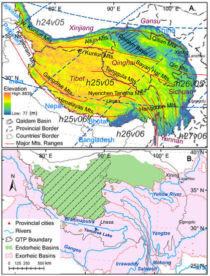
Figure 1.
Study Area of Qinghai-Tibetan Plateau (QTP): (A) elevation, major Mts. (i.e., mountains) ranges, and provincial and country borders; (B) provincial cities, rivers, and the endorheic and exorheic basins. The grids, in dark blue dashed lines, overlaid are the corresponding MODIS tiles (e.g., h25v06). Boundaries of Changtang Plateau (shadowed with the dashed lines in (B) and the endorheic, and exorheic basins were determined from the 15-s HydroSHEDS (Hydrological data and maps based on SHuttle Elevation Derivatives at multiple Scales) drainage basin dataset [42]. Map created using ArcGIS 10.6 (ESRI, CA, www.esri.com).
2.2. LCLU Mapping
The mapping of LCLU in QTP generally followed our previous work in Northern China [27,35] with adaptation to this study region. Specifically, to acquire the predictors for mapping the land-cover, we used the MODIS (Moderate Resolution Imaging Spectroradiometer) vegetation indices’ (VI) product (MOD13Q1, 16-day Level 3 Global 250-m Sinusoidal Grid, Collection 5), which were stored in an HDF (Hierarchical Data Format) file with the MODIS Sinusoidal sphere-based projection. Our study area of QTP was mainly covered by 6 MODIS tiles, H24V05, H25V05, H26V05, H25V06, H26V06, and H27V06 (dark blue dashed grids in Figure 1A). We collected all scenes (n = 6 × 23 scenes/y × 16 y − 18 missing scenes = 2190 scenes) of these 6 tiles from 2000–2015 at each 16-day interval. Each scene of the MOD13Q1 VIs’ product included normalized difference vegetation index (NDVI), enhanced vegetation index (EVI), blue, red, near-infrared (NIR), mid-infrared (MIR) reflectance, and pixel summary quality assurance (QA) variables. The image preprocessing steps were completed with a set of scripts in the IDL programming language, which implemented the user functions of the ENVI/IDL software, as well as an ENVI/IDL plugin named the MODIS Conversion Toolkit. We drew the flowchart on processing predictor variables in Figure A1 (Appendix A). After extracting each variable from these tiles for each date, we conducted image mosaicking and then reprojected to the Albers Conic Equal Area projection (central longitude of 105°E, two standard parallels of 27°N and 45°N latitudes, and center latitude of 35°N) for each date using the nearest neighbor resampling approach. Based on the extracted time series of variables from MOD13Q1, we derived the growing season (from the 97th–289th day of the year), the statistics of the mean, standard deviation, minimum, maximum, and range of VIs, and the reflectance of blue, red, near-infrared, and mid-infrared bands, which were used together with the four-season (every three months from December of the last year to November of the target year) VIs’ statistics, to classify LCLU for each calendar year from 2001–2015. The QA variable was used to mask out no data (i.e., QA equals −1) and cloudy (i.e., QA equals 3) pixels prior to calculating statistics. In addition to the aggregated statistics, we calculated the vegetation phenological parameters for each year of the study period (from 2001–2015) based on a 16-year time series of MODIS EVI from 2000–2015 with the software package of TIMESAT (Version 3.1) [43], because the TIMESAT program applies QA-adjusted weights on EVI to derive phenological parameters in the growing season of the target year according to both EVI and the QA series of the target year and the adjacent years. We used the starting date, mid-season date, growing season length, base, peak, and amplitude of EVI, the rates of increase at the beginning and decrease at the end of a season, and the seasonal integrals of EVI from the derived phenological parameters as predictors for further classification.
Considering the important roles of terrain variables in determining vegetation distributions, we also included elevation, slope, and aspect derived from the Shuttle Radar Topography Mission Digital Elevation Model (SRTM 90 m DEM Version 4) with missing data filled by the Consultative Group for International Agriculture Research [44].
Following the rules of the sampling criteria in the relevant literature and the visual interpretation schema of our previous studies [27,35], we collected 5276 ground reference points covering 14 land-cover types, i.e., deciduous broadleaved forest (DBLF), evergreen broadleaved forest (EBLF), evergreen needle-leaved forest (ENLF), mixed forest (MIXF), closed shrubland (CLSH), open shrubland (OPSH), meadow (MEDO), steppe (STEP), sparse vegetation (SPAS), urban area (URBN), agricultural land (AGRI), bare ground (BARE), permanent snow cover (SNOW), and water (WATR) by means of a semi-random method. Specifically, to collect the ground reference points, we first randomly generated points based on the criteria that the distance between any pair pixels was greater than 1500 m to minimize the spatial autocorrelation and the effects of triangular PSF (point spread function) along the scan direction of the MODIS sensor [36]. Then, the ground reference points were identified through visualized interpretation with the aid of the historical vegetation maps [45], the high-resolution images, and user-pinned photos on Google Earth (GE), the species distribution information from Flora of China (www.efloras.org), and the ground observations at the field stations of the Chinese Ecological Research Network (CERN, www.cern.ac.cn). To avoid mixed land type reference points located on spatial heterogeneous areas, we also made sure each reference point as a MODIS pixel was located within a uniform land-cover patch on GE imagery during the process of reference identification. The sampling points of different years were also considered based on high-resolution GE imagery available for different years. To facilitate ground reference points’ collection, we created a sample collection reference table, which listed the ground photographs (available at GE or CERN), typical high-resolution GE images, and a brief description of the locations for these LCLU types within QTP (Supplementary Table S1).
Based on the acquired ground reference points, we extracted the training dataset with the abovementioned variables and then randomly divided them into two subsets: 70% for training the classifier and the rest for the independent validation. We built a land-cover classification model by means of the “random forests” (RF) classifier [46] with the “randomForest” package provided by the open source statistical software R [47] since the RF classifier has been proven to achieve high classification accuracy and robust and efficient performance [27,35]. We set up the parameters of the RF classifier (i.e., mtry of 6 and ntree of 500) using tuning functions according to the overall accuracy and the efficiency. Based on the training subset, we formed three combination groups of predictors as the training inputs to build three classification models (i.e., G1 encompassed all the predictors; G2 included the growing season statistics of reflectance and VIs, the phenology parameters, and the topographical variables; G3 was a modification of G2 by substituting four-season statistics of VIs for the phenology parameters).
The accuracies of classification models were evaluated using overall classification accuracy (OA), producer’s accuracy (PA), user’s accuracy (UA), and Kappa statistics. We found that the model constructed with all predictors achieved the highest classification accuracy, which was consistent with our previous studies. Thus, we applied the classification model built with G1 predictors to the whole QTP to produce annual land-cover maps, as well as the class membership probability datasets at the pixel level for each year from 2001–2015.
2.3. LCLUC Spatial Pattern Analysis
Land cover maps derived from satellite images were sensitive to the fluctuations of ecosystems states, and it is problematic if land-cover changes during a specific period are computed as the difference between the two ends [48,49]. In this study, we adopted the hotspot analyses used by Wang et al. [35] to quantify land conversions among AGRI, BARE, CLSH, FORE (including all forest types), GRAS (steppe and meadow), OPSH, SPAS, URBN, and WATR during the study period. Specifically, we counted the percentages of the nine grouped land-cover types in each large grid cell of 2.5 × 2.5 km2 (10 × 10 MODIS pixels) to minimize the effect of “speckle” in land-cover maps and acquired time series of land-coverage for each land-cover type at each large cell. To obtain an unbiased estimation of temporal trends in land-cover, we regressed the land-coverage in the time series on time and estimated the slope. The significant slopes (p-value < 0.1) were multiplied by the time period to quantify the mean change of each land-cover type, and the corresponding standard errors were also multiplied by the time period to estimate the uncertainty in net land-cover change. According to the estimated LC gain/loss, the maps of land-cover change at the large-grid level were obtained, and LCC hotspots were identified. We then explored the interrelationships among the spatial patterns of deforestation, reforestation, agriculture abandonment and reclamation, grassland degradation, and surface water expansion by calculating the areas of net land transfer among the land-cover types within QTP.
2.4. Environmental and Anthropogenic Forcing
To explore environmental forcing and human activities on LCLUC, we collected the following variables. Due to a limited number of meteorological stations, we acquired the monthly daytime land surface temperature (DLST) and nighttime land surface temperature (NLST) datasets from the gridded land surface temperature global product (MOD11C3, Collection 6) at a 0.05° spatial resolution produced with spatiotemporal gap-filling and aggregation. The monthly precipitation was extracted from the daily gridded rainfall product at 0.05° spatial resolution, provided by the Climate Hazards group Infrared Precipitation with Stations (CHIRPS) dataset Version 2.0 [50]. The monthly evapotranspiration (ET) was derived from the Evapotranspiration/Latent Heat Flux product (MOD16A2, Collection 6) with 500-m spatial resolution [51]. The monthly climate data were aggregated to annual mean time series. After reprojection and resampling, we estimated the temporal trends (slope as the rate of change) of these four climate variables using the method of “AAT” (i.e., trends on annual aggregated time series) implemented in the green-brown R package [52]. To represent the anthropogenic activities, the changes in population density between 2000 and 2015 were extracted from the Gridded Population of the World (Version 4) [53].
3. Results
3.1. Accuracy of LCLU Mapping
According to the confusion matrix (Table 1), the overall accuracy and Kappa statistics of our land-cover classification were 82.2% and 78.7%, respectively. The classification accuracies (both PA and UA) of SNOW, WATR, and BARE were greater than 90%; URBN, ENLF, and AGRI had both accuracies greater than 85%. The accuracy of grouped forests (FORE) in QTP, including DBLF, EBLF, ENLF, and MIXF, achieved an average PA of 91.5% and UA of 95.4%. The omission errors of MEDO and AGRI were 10.3% and 13.6%, respectively, mostly due to similar spectral characteristics among MEDO, AGRI, and CLSH. There existed a large omission error of 77.4% for MIXF, mostly due to the irregular spectral features caused by heterogeneous mixture of coniferous and broadleaved trees and the complex altitudinal distribution of MIXF in the steep-slope environment (with an average of 25°). OPSH with a PA of 53.8% was likely to be misrecognized as MEDO, CLSH, SPAS, and STEP. The omission error of CLSH was 34.3%, mainly because of the confusion with MEDO.

Table 1.
Confusion matrix of the classification (UA, user’s accuracy; PA, producer’s accuracy; OA, overall accuracy; Kappa, Kappa statistics; AGRI, agricultural land; BARE, bare ground; CLSH, closed shrubland; DBLF, deciduous broadleaved forest; EBLF, evergreen broadleaved forest; ENLF, evergreen needle-leaved forest; MIXF, mixed forest; MEDO, meadow; OPSH, open shrubland; SNOW, permanent snow cover; STEP, steppe; SPAS, sparse vegetation; URBN, urban area; and WATR, water).
3.2. Patterns and Hotspots of Land-Cover Change in QTP during 2001–2015
Net change: During 2001–2015, QTP witnessed remarkable LCLU changes (Figure 2). Agricultural land and permanent snow/ice shrank by 5850.3 km2 (about a −5.1% reduction) and 8894.1 km2 (−3.4%), respectively. Bare ground and meadow decreased substantially with net losses of 20,676.8 km2 (−2.8%) and 22,968.8 km2 (−4%), respectively. Net loss of these land-cover types was mostly due to expansion of FORE, steppe, closed/open shrubland, sparse vegetation, and water. In particular, FORE and closed shrubland significantly expanded with a net gain of 13,111 km2 (4.8%) and 8952.4 km2 (5.7%), respectively. Likewise, steppe, sparse vegetation, and open shrubland increased by 9660.6 km2 (2.4%), 10,413.4 km2 (2%), and 9342.3 km2 (21%), respectively. There was a noticeable increase of 5866.4 km2 (10.2%) in water surface. Urban areas also expanded 585.7 km2 at a rate of 41.2%.
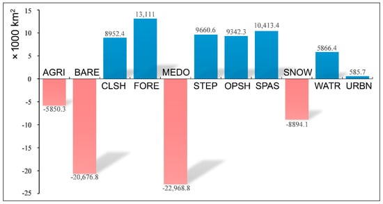
Figure 2.
Land cover net gain and net loss in the Qinghai-Tibetan Plateau. FORE stands for all forest types; AGRI, agricultural land; BARE, bare ground; CLSH, closed shrubland; MEDO, meadow; OPSH, open shrubland; SNOW, permanent snow cover; STEP, steppe; SPAS, sparse vegetation; URBN, urban area; and WATR, water.
Forest and closed-shrubland change hotspots: The spatial patterns of forest change from 2001–2015 concentrated in the southeast such as the southeastern Qin Mountains, the Hengduan Mountains, the southern Nyenchen Tanglha Mountains, and the eastern edge of the Himalayas (Figure 1A and Figure 3A). Forest expansion mainly happened in the previous closed shrubland, meadow, and agricultural land (Figure 3). Closed shrubland also expanded towards the Central Plateau at the expense of decreased meadow (Figure 3B,C). In particular, the forest gain of 16,295.3 km2 mostly came from the losses of closed shrubland (5523.8 km2), meadow (3963.3 km2), and agriculture land (3954.8 km2). Forest loss of 3183.7 km2 was mostly converted to closed shrubland (1594.8 km2), agriculture land (714.4 km2), and open shrubland (397.7 km2).
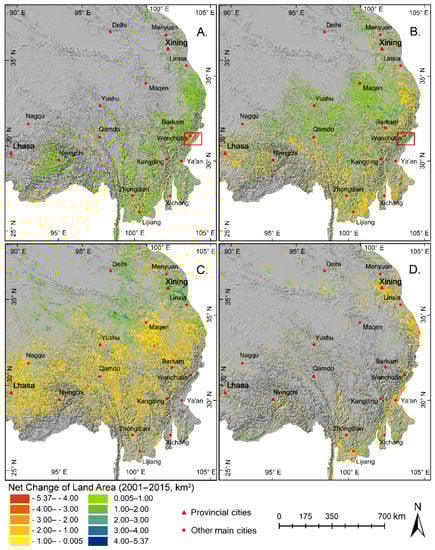
Figure 3.
Net changes of (A) forest, (B) closed shrubland, (C) meadow, and (D) agriculture from 2001–2015. The red box in (A,B) indicates the forest habitats destroyed by the earthquake in 2008. Land changes are significant with a p-value < 0.1.
Agricultural abandonment and reclamation: We also found the decline of agricultural land (8765.2 km2) in the eastern QTP during 2001–2015 (Figure 3D), and the loss was mainly associated with the expansion of forest (4634 km2) in the eastern mountains and meadow (1764.4 km2) near the provincial city Xining. To a lesser extent, agricultural lands were converted to open shrubland (561.1 km2), urban area (232.6 km2), and water (325.6 km2). On the other hand, new agricultural lands were also found for some patches in the eastern QTP (Figure 3D). In southeastern Qaidam Basin (Figure 1A), the patches with gains in agricultural land approximately corresponded to the areas with loss in sparse vegetation (605.7 km2) and bare ground (257.6 km2) (Figure 4C,D). While in southern and southeastern QTP, the gains in agricultural land mainly came from the forest (927.7 km2), meadow (369.2 km2), and closed shrubland (266.4 km2).
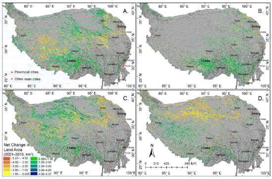
Figure 4.
Sparse vegetation changes are associated with bare ground and grassland. Net changes of (A) steppe, (B) open shrubland, (C) sparse vegetation, and (D) bare ground from 2001–2015. Land changes are significant with a p-value < 0.1.
Grassland change: The meadow in the southeastern QTP (Figure 3C) declined significantly and was mostly converted to closed shrubland (13,805 km2), steppe (7562.9 km2), forest (5027.5 km2), open shrubland (4880 km2), and sparse vegetation (1670.3 km2) (Figure 3 and Figure 4). Contrary to the meadow loss in the southeast, the meadow in northeast QTP expanded (Figure 3C) into steppe (−7396.7 km2), sparse vegetation (−2363.1 km2), agricultural land (−2557.5 km2), and closed shrublands (−776.8 km2). The steppe gain appeared in two clusters (Figure 4A). One was in the vicinity of the three adjacent cities (i.e., Lhasa, Nagqu, and Nyingchi), and the net gain of steppe was accompanied by a massive decline of meadow (−9126 km2) and glacier (−3050 km2). The other was located near the border of the Qaidam Basin (Figure 1A and Figure 4A), where open shrublands also increased by 1143 km2, but sparse vegetation and bare ground loss by 16,620 and 1725 km2, respectively. The steppe loss hotspots also mainly concentrated in two areas. One was in the outer edges around the Qaidam Basin due to the enormous meadow expansion of 8646 km2 (Figure 3C and Figure 4A). The other hotspot of steppe loss was in western Tibet between the cities of Ga’er and Nagqu where steppe was mainly converted to sparse vegetation (9832 km2) and bare ground (1332) (Figure 4A,C,D). In summary, the grassland (i.e., steppe and meadow) changes were highly spatially heterogeneous. The loss was mainly converted into closed/open shrubland, forest, and sparse vegetation, while the grassland gains were mainly from sparse vegetation, glacier, and agricultural land.
Loss of permanent snow/ice (glaciers): The massive glacier loss mainly occurred in the south and southeast, especially in the Ganges-Brahmaputra river basin (Figure 1B and Figure 5A). Where the glacier loss, bare ground, sparse vegetation, steppe, and open shrubland increased substantially by 2638.7, 2192.3, 1821.8, and 667.5 km2, respectively. Meanwhile, forest and closed shrubland gained by 477.4 km2 and water surface by 128 km2, while meadow lost by 1067 km2. On the contrary to the massive loss, spots with glacier gain were scarce and scattered (Figure 5A). In these spots, glaciers and water expanded by 100 and 225 km2, respectively, together with the shrinkage of bare ground (−571 km2).
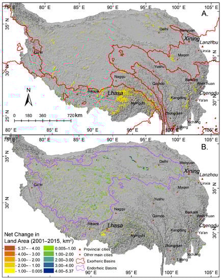
Figure 5.
Spatial patterns of net changes in (A) permanent snow and ice and (B) surface water bodies. Land changes are significant with a p-value < 0.1.
Expansion of surface water bodies: The surface water changes were mainly distributed in the endorheic basins (Figure 1B and Figure 5B), especially on the Changtang Plateau. Continued expansion of the water drowned the vast areas of bare ground (−5113.7 km2), sparse vegetation (−1279.2 km2), grassland (−660.0 km2), and agricultural land (−360.8 km2). There were also many small water-gain clusters around Nyingchi near the mountains of Hengduan, Nyenchen Tanglha, and the eastern edge of the Himalayas (Figure 1A and Figure 5B), where large patches of glaciers were distributed on the top of these mountains. The small water-gain clusters here were associated with the loss of glacier (−283.8 km2, Figure 5). Water loss occurred in many small patches in the west and center of the endorheic basins (Figure 5B). There were also several large patches with surface water retreat along Yamdrok Lake and Brahmaputra River in the south of Lhasa (Figure 1B and Figure 5B). As a result, the bare ground, sparse vegetation, and steppe advanced into these patches by 803.0, 444.4, and 295.9 km2, respectively.
4. Discussion
4.1. Economy Shift, Conservation Policy, and Agricultural Lands’ Change
Agricultural land reduction was mainly a result of conservation policies and, to a lesser extent, expansion of urban areas. Different from the flat cultivated land in eastern China, the agriculture in the southeastern QTP can be called “valley agriculture” because most (65%) of the cultivated lands occur in the high-elevation (>2500 m) river valley plains (i.e., Huangshui River, Minjiang River, Dadu River, and Brahmaputra River) [20]. These valleys meet the temperature and the light required for crop growth, as well as the topographical condition for tillage and irrigation. However, the agricultural outputs of most QTP farmlands are low because the farmlands are surrounded by rolling mountains and are vulnerable to erosion [54]. To complement the low income from agricultural production, farmers and herdsmen often make earnings from other non-cropping activities such as livestock farming [20,55]. Since 2000, the national environmental protection policies have been implemented in most of China and covered more than 67.6% of QTP (Figure A3B). As a result, a total of 155 protected reserves have been established in QTP, accounting for 32.4% of the total area [56,57]. Consequently, many croplands, especially those marginal for agriculture, were converted into woodland or grassland via natural succession or plantation. For instance, the decline of agricultural land in the areas between Xining and Linxia in the northeast was partially driven by the policy of returning farmland to forest and grassland (Figure 3D and Figure A3B) and the related changes in human population (Figure A3A).
The special natural settings of QTP and recent rapid growth of the transportation infrastructure have promoted the booming of tourism (e.g., 29.9% of Tibet’s GDP in 2016) [56,58,59]. As a result, economic development has absorbed more and more agricultural laborers into urban areas [60]. This is reflected in the population change (Figure A3A): during 2000–2015, the urban population growth rate, with an average of more than 15 persons/km2, was much higher than the rural population growth of 0–3 persons/km2. Similar to many other regions in China, rural-urban migration has driven the development of urbanization in QTP, and urban expansion is mostly converted from farmland near the major cities [35].
4.2. Conservation, Climate Change, and Woodland Expansion into Grassland
Climate warming and overgrazing are two major threats to alpine grasslands, which account for about 50% of the whole plateau area and 44% of the total grassland area in China [32,61]. Warming can convert marginal grassland to desert and reduce the ecosystem stability [62] by producing less biomass in dry years, but more biomass in wet years. Overgrazing severely decreases the surface biomass and creates soil heterogeneity [63]. Overgrazing and warming-induced instability are believed to be the two major causal factors that lead to shrub encroachment into grasslands [64,65]. It was reported that from 1990–2009, about 39% of the alpine meadow in the northwest Yunnan was converted to woody shrubland [18]. We found that during 2001–2015, alpine meadow in QTP sharply decreased by 23 × 103 km2. The loss of alpine meadow was mostly in the southeast, and approximately 72% of the loss was converted to shrublands (closed and open) and forests. Warming and overgrazing may also lead to the conversion of meadow to dry steppe, as we showed that 23% of the meadow loss in the southeast became dry steppe. Closed shrublands in the southeast also became forests via succession (Figure 3A,B), especially in the eastern boundary favored by increased precipitation (Figure 6C).
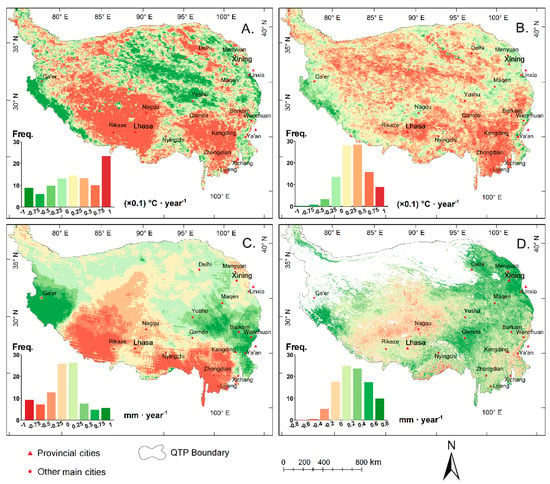
Figure 6.
Spatial patterns of the trends of (A) annual mean land surface temperature at daytime, (B) annual mean land surface temperature at nighttime, (C) annual mean precipitation, and (D) annual mean evapotranspiration in 2001–2015 (maps and histograms were created using ArcMap 10.6).
In areas with increased rainfall, such as the southern outermost edge of Qaidam Basin in the northern QTP, the alpine meadow was expanding on the land that was originally sparse vegetation and alpine steppe (Figure 3C, Figure 4A,C and Figure 6C). For the same reason, alpine steppe gained from originally vegetation and desert around the southern boundary of Qaidam Basin (Figure 4A), and the sparse vegetation appeared in the eastern Kunlun Mountains due to the restoration (Figure 4C,D). The above results indicated that the ecological environment in the above areas shifted towards a positive direction, which was partially driven by the increased precipitation (Figure 6C) and the implementation of conservation policies (Figure A3B), such as the Reduce Grazing Return Grasslands Project under the “Grain for Green Program” and the Conservation and Restoration of the Qilian Mountain ecosystem Project under the “Natural Forest Conservation Program”. Lehnert, Wesche, Trachte, Reudenbach, and Bendix [16] illustrated a similar view that the significant increase of vegetation cover between 2000 and 2013 was primarily driven by the positive precipitation trend in the regions of southern and eastern Qinghai. However, the alpine steppe and sparse vegetation were degraded to barren land around the areas between Nagqu and Ga’er (the prefectures of Nagqu and Nagari) in the western QTP (Figure 4). This illustrated that the climatic conditions in the western plateau are not favorable to the growth of vegetation (Figure 6A,C,D). The degradation of grassland and sparse vegetation to barren land in arid areas of the western Qinghai-Tibet Plateau is closely related to the worsening drought due to the strong increasing trend of daytime and nighttime temperature during the past decades (Figure 6A,B) [17,31].
Conservation policies may also play an important role in shrubland and forest expansion in QTP. The eastern QTP historically experienced an unprecedented deforestation due to the modern commercial timber production [22,66], especially since the late 1950s in the eastern Himalayas and the Hengduan mountains [25,40]. The degradation of forest and shrub ecosystems led to the decline of the ecosystem function and service and resulted in damage or even the collapse of the entire system [67,68]. Conservation policy implementation started in the late 1980s. The central government successively promulgated the laws of Forest and Prairie and implemented them as “the Shelterbelt Development Program” to promote the restoration of ecosystems for soil and water conservation in the middle and upper reaches of Yangtze River. Additionally, many nature reserves such as key ecological function areas and national ecological security barrier areas have been identified and established rapidly in recent decades [26], which has played a positive role in the ecological protection and restoration in QTP. Especially since 2000, the Chinese government has implemented a series of environmental protection policies and afforestation and reforestation programs such as the “Grain for Green” and “Natural Forest Conservation” programs [26,35,69]. Our results showed that the area where the policies were implemented matched with the area of woodland expansion (Figure 3A,B and Figure A3B). Our results also revealed a forest loss hotspot caused by a natural disturbance, i.e., the Wenchuan earthquake in May 2008, which destroyed many forest habitats (red box in Figure 3A). These areas were then regenerated into shrublands (red box in Figure 3B).
4.3. Increased Precipitation/Warming and Water Surface Expansion/Glacier Retreat
Global studies showed that the endorheic lakes in all the regions in the world have been expanding in the last 30 years, and the mean rate of expansion was estimated as 390 km2 y−1 for the Tibetan Plateau [70,71]. In this paper, we found that QTP gained 5866.4 km2 of new surface water area, which was slightly larger than the 5460 km2 calculated from the rate of 390 km2 y−1. The difference might be due to different image source (MODIS versus Landsat images), spatial resolution, and/or classification methods [49]. The long-term trend of terrestrial water storage (TWS) derived from the Gravity Recovery and Climate Experiment (GRACE) illustrated that TWS presented two clusters in QTP during 2003–2015 (Figure A2). This clearly shows that TWS increased in most of the endorheic basin (i.e., bounded with purple color) with a mean of approximately 0.59 ± 0.65 mm y−1. This could be partly linked to the expansion of surface water due to the increase of precipitation (Figure 6C) in the endorheic basin [9,72,73]. Small patches with water surface expansion also appeared in the northeastern QTP, which might be caused by both the dam impounding for hydroelectric power in the upper reaches of the Yellow River and the precipitation increase (Figure 6C) [74].
Contrary to the expansion of surface water in the endorheic basin, the mountain glaciers in the southern QTP retreated (Figure 5A), which is consistent with recent reports [75,76]. Both daytime and nighttime temperatures showed increasing trends in the southeastern QTP (Figure 6A,B). The melting of glacier and ice is reported to relate to the steep rise in temperature [77], and the extent of glacier shrinkage is projected [7,76]. Additionally, the deposition onto the glaciers of light-absorbing aerosol particles such as dust and black carbon could accelerate glaciers’ melting due to the darkening effect [78] and the reduced albedo, which act to absorb more solar radiation [1,3,79]. The rapid glacier melting and recent drought also led to the shrinkage of TWS [80]. For example, TWS in the southeastern QTP decreased with a mean of approximately −1.36 ± 0.62 mm y−1 during 2003–2015 (Figure A2). Continued warming is expected to melt the glaciers and thaw the permafrost, which might accelerate the hydrological processes in this “water tower of Asia” [81]. The rapid melting of glaciers in early spring could trigger water scarcity in early summer and exert great pressure on humans of many countries in Asia [16,82].
5. Conclusions
The land-cover changes during 2001–2015 are highly spatially heterogenous across the plateau. Woodlands experienced substantial expansion in the southeast with the expansion of meadow shrinkage, mostly driven by conservation policies, warming, or/and overgrazing. Policies on returning farmlands to forests and grasslands for soil and water conservation mostly drive the agricultural land conversion. Increased precipitation promotes the expansion of surface water in the center and east of the endorheic basins, as well as the local expansions of meadow, steppe, and sparse vegetation. Warming in the south and the southeast melts the mountain glaciers and, together with drought, leads to the shrinkage of terrestrial water storage in the southeast. Continued warming is expected to melt the glaciers and thaw the permafrost, which might accelerate the hydrological cycles and modify the carbon cycles, thus complicating the responses and feedbacks of the alpine ecosystems to global change. The substantial changes in land-cover reveal the high sensitivity of QTP to changes in climate and human activities. Rational policies for conservation might mitigate the adverse impacts to maintain essential services provided by the important alpine ecosystems.
At a broad level, land-use-cover change, human activities, and climate change are closely related as they have causal relationships. By analyzing the spatial patterns of LCLUC in QTP and exploring the possible causes and effects, this study highlighted the joint impacts of human decision-making and natural biophysical processes on ecosystems. For example, climate change plays a leading role in the west of QTP, while human economic development, environmental protection policies, and climate change play a joint role in the east. The methods adopted in this study could be used for quantifying LCLUC in other mountainous regions, and the discussions on potential factors driving LCLUC set a sound base for further LCLUC modeling to support decision-making on ecological conservation policies for sustainable development.
Supplementary Materials
The following are available online at https://www.mdpi.com/2072-4292/11/20/2435/s1, Table S1: Landscape photographs and descriptions of land-cover types, adapted from Wang et al., 2016. Photographs were acquired from Google Earth photos near some reference points.
Author Contributions
Conceptualization, Q.G. and M.Y.; methodology, Q.G. and M.Y.; formal analysis, C.W.; investigation, C.W., Q.G., and M.Y.; data curation, C.W.; writing, original draft preparation, C.W.; writing, review and editing, Q.G. and M.Y.; supervision, Q.G. and M.Y.; project administration, M.Y.; funding acquisition, Q.G. and M.Y.
Funding
This research was funded by the starting fund from the University of Puerto Rico, Rio Piedras.
Acknowledgments
This work was supported by the starting fund from the University of Puerto Rico, Rio Piedras. We acknowledge NASA for providing the MODIS data, SRTM DEM, and the Gridded Population of the World dataset, NASA Goddard Space Flight Center for providing GRACE mascon data, and the Google Earth Engine for the preprocessing dataset. We also thank Di Dong, Xianbin Liu, Loderay Bracero Marrero, Marianne Cartagena-Colón, Xian Wang, Fangfang Yao, and Kehan Yang for their feedback on an earlier version.
Conflicts of Interest
The authors declare no conflict of interest. The funders had no role in the design of the study; in the collection, analyses, or interpretation of data; in the writing of the manuscript; nor in the decision to publish the results.
Appendix A

Figure A1.
Flowchart on processing predictor variables. QA, quality control; VI, vegetation indices; EVI, Enhanced Vegetation Index; Squares, source data and processed data; Diamonds, operations; Arrows, processing directions.
Spatial patterns of terrestrial water storage anomalies trend
Due to the important roles surface water bodies and glaciers play in the regional hydrologic cycle, terrestrial ecosystems, and climate change over QTP, we explored the spatial patterns of the variations in terrestrial water storage (TWS) over QTP based on the satellite gravity mass anomalies’ data at high-temporal resolution provided by the Gravity Recovery and Climate Experiment (GRACE) mission since the spring of 2002. The variations of TWS were sensitive to fluctuations in both event flow (precipitation-driven) and base flow (stored in ice sheets, soil, and groundwater) [83,84]. We acquired the latest release of the GRACE global monthly mass concentration blocks (mascons) Version v02.3 with the correction of the glacial isostatic adjustment model from the NASA Goddard Space Flight Center (GSFC) [85]. On land and ice cover area, the mascon primarily describes the total variability in water content after the removal of atmospheric and oceanic effects [86]. For each mascon, this product contains the time-variable gravity monthly time series with the removal of the mean over the span of years from 2004 to 2016 in terms of cm equivalent water height and the associated time-dependent uncertainties (the detailed description of the GSFC mascon estimation procedure refers to Luthcke, Rowlands, Sabaka, Loomis, Horwath, and Arendt [83]). We estimated the temporal trend of GRACE-derived TWS anomalies using the same method as the trend estimation of climate variables in Section 2.4 [52].

Figure A2.
Spatial patterns of the trends of annual mean TWS anomalies from 2003–2015 (the trend was calculated using the R statistical software; maps and histograms were created using ArcMap 10.6, ESRI, CA).

Figure A3.
(A) Population density change (i.e., Pop. Dens. Ch. (indiv./km2) means the population density change at the unit of individuals per square kilometer) between 2000 and 2015, derived from population density data acquired from the Gridded Population of the World, Version 4 (GPWv4) collection; (B) two main ecological restoration programs in QTP (GFG, Grain for Green Program, NFCP, Natural Forest Conservation Program).
References
- Qiu, J. The third pole. Nature 2008, 454, 393–396. [Google Scholar] [CrossRef] [PubMed]
- Yanai, M.; Li, C.; Song, Z. Seasonal heating of the Tibetan Plateau and its effects on the evolution of the Asian summer monsoon. J. Meteorol. Soc. Jpn. Ser. II 1992, 70, 319–351. [Google Scholar] [CrossRef]
- Wu, G.X.; Liu, Y.M.; He, B.; Bao, Q.; Duan, A.M.; Jin, F.F. Thermal controls on the Asian summer monsoon. Sci. Rep. 2012, 2, 404. [Google Scholar] [CrossRef] [PubMed]
- Funnell, D.; Parish, R. Mountain Environments and Communities; Routledge: London, UK, 2005; p. 432. [Google Scholar]
- Kutzbach, J.E.; Prell, W.L.; Ruddiman, W.F. Sensitivity of Eurasian climate to surface uplift of the Tibetan Plateau. J. Geol. 1993, 101, 177–190. [Google Scholar] [CrossRef]
- Zhang, L.; Su, F.; Yang, D.; Hao, Z.; Tong, K. Discharge regime and simulation for the upstream of major rivers over Tibetan Plateau. J. Geophys. Res. Atmos. 2013, 118, 8500–8518. [Google Scholar] [CrossRef]
- Bolch, T.; Kulkarni, A.; Kääb, A.; Huggel, C.; Paul, F.; Cogley, J.G.; Frey, H.; Kargel, J.S.; Fujita, K.; Scheel, M.; et al. The state and fate of Himalayan glaciers. Science 2012, 336, 310–314. [Google Scholar] [CrossRef]
- Immerzeel, W.W.; van Beek, L.P.H.; Bierkens, M.F.P. Climate change will affect the Asian water towers. Science 2010, 328, 1382–1385. [Google Scholar] [CrossRef]
- Lei, Y.; Yang, K. The cause of rapid lake expansion in the Tibetan Plateau: Climate wetting or warming? Wiley Interdiscip. Rev. Water 2017, 4, e1236. [Google Scholar] [CrossRef]
- Myers, N.; Mittermeier, R.A.; Mittermeier, C.G.; da Fonseca, G.A.B.; Kent, J. Biodiversity hotspots for conservation priorities. Nature 2000, 403, 853–858. [Google Scholar] [CrossRef]
- Marchese, C. Biodiversity hotspots: A shortcut for a more complicated concept. Glob. Ecol. Conserv. 2015, 3, 297–309. [Google Scholar] [CrossRef]
- Yao, T.; Thompson, L.; Yang, W.; Yu, W.; Gao, Y.; Guo, X.; Yang, X.; Duan, K.; Zhao, H.; Xu, B.; et al. Different glacier status with atmospheric circulations in Tibetan Plateau and surroundings. Nat. Clim. Chang. 2012, 2, 663–667. [Google Scholar] [CrossRef]
- Song, Y.; Jin, L.; Wang, H. Vegetation changes along the Qinghai-Tibet Plateau engineering corridor since 2000 induced by climate change and human activities. Remote Sens. 2018, 10, 95. [Google Scholar] [CrossRef]
- Piao, S.; Cui, M.; Chen, A.; Wang, X.; Ciais, P.; Liu, J.; Tang, Y. Altitude and temperature dependence of change in the spring vegetation green-up date from 1982 to 2006 in the Qinghai-Xizang Plateau. Agric. For. Meteorol. 2011, 151, 1599–1608. [Google Scholar] [CrossRef]
- Xu, Z.X.; Gong, T.L.; Li, J.Y. Decadal trend of climate in the Tibetan Plateau—Regional temperature and precipitation. Hydrol. Process. 2008, 22, 3056–3065. [Google Scholar] [CrossRef]
- Lehnert, L.W.; Wesche, K.; Trachte, K.; Reudenbach, C.; Bendix, J. Climate variability rather than overstocking causes recent large scale cover changes of Tibetan pastures. Sci. Rep. 2016, 6, 24367. [Google Scholar] [CrossRef]
- Wang, M.; Zhou, C.; Wu, L.; Xu, X.; Ou, Y. Wet-drought pattern and its relationship with vegetation change in the Qinghai-Tibetan Plateau during 2001–2010. Arid Land Geogr. 2013, 36, 49–56. [Google Scholar]
- Brandt, J.S.; Haynes, M.A.; Kuemmerle, T.; Waller, D.M.; Radeloff, V.C. Regime shift on the roof of the world: Alpine meadows converting to shrublands in the southern Himalayas. Biol. Conserv. 2013, 158, 116–127. [Google Scholar] [CrossRef]
- Chen, B.; Zhang, X.; Tao, J.; Wu, J.; Wang, J.; Shi, P.; Zhang, Y.; Yu, C. The impact of climate change and anthropogenic activities on alpine grassland over the Qinghai-Tibet Plateau. Agric. For. Meteorol. 2014, 189, 11–18. [Google Scholar] [CrossRef]
- Paltridge, N.; Tao, J.; Unkovich, M.; Bonamano, A.; Gason, A.; Grover, S.; Wilkins, J.; Tashi, N.; Coventry, D. Agriculture in central Tibet: An assessment of climate, farming systems, and strategies to boost production. Crop Pasture Sci. 2009, 60, 627–639. [Google Scholar] [CrossRef]
- Feddema, J.J.; Oleson, K.W.; Bonan, G.B.; Mearns, L.O.; Buja, L.E.; Meehl, G.A.; Washington, W.M. The importance of land-cover change in simulating future climates. Science 2005, 310, 1674–1678. [Google Scholar] [CrossRef]
- Cui, X.; Graf, H.-F. Recent land-cover changes on the Tibetan Plateau: A review. Clim. Chang. 2009, 94, 47–61. [Google Scholar] [CrossRef]
- Liu, J.; Dietz, T.; Carpenter, S.R.; Folke, C.; Alberti, M.; Redman, C.L.; Schneider, S.H.; Ostrom, E.; Pell, A.N.; Lubchenco, J. Coupled human and natural systems. AMBIO J. Hum. Environ. 2007, 36, 639–649. [Google Scholar] [CrossRef]
- Verburg, P.H.; Neumann, K.; Nol, L. Challenges in using land use and land-cover data for global change studies. Glob. Chang. Biol. 2011, 17, 974–989. [Google Scholar] [CrossRef]
- Chen, H.; Zhu, Q.; Peng, C.; Wu, N.; Wang, Y.; Fang, X.; Gao, Y.; Zhu, D.; Yang, G.; Tian, J.; et al. The impacts of climate change and human activities on biogeochemical cycles on the Qinghai-Tibetan Plateau. Glob. Chang. Biol. 2013, 19, 2940–2955. [Google Scholar] [CrossRef] [PubMed]
- Zheng, Z.; Zeng, Y.; Zhao, Y.; Gao, W.; Zhao, D.; Wu, B. Analysis of land-cover changes in southwestern China since the 1990s. Acta Ecol. Sin. 2016, 36, 7858–7869. [Google Scholar] [CrossRef][Green Version]
- Wang, C.; Gao, Q.; Wang, X.; Yu, M. Decadal trend in agricultural abandonment and woodland expansion in an agro-pastoral transition band in northern China. PLoS ONE 2015, 10, e0142113. [Google Scholar] [CrossRef] [PubMed]
- Gao, Q.; Yu, M. Discerning fragmentation dynamics of tropical forest and wetland during reforestation, urban sprawl, and policy shifts. PLoS ONE 2014, 9, e113140. [Google Scholar] [CrossRef]
- Ding, M.; Zhang, Y.; Shen, Z.; Liu, L.; Zhang, W.; Wang, Z.; Bai, W.; Zheng, D. Land cover change along the Qinghai-Tibet Highway and Railway from 1981 to 2001. J. Geogr. Sci. 2006, 16, 387–395. [Google Scholar] [CrossRef]
- Lu, J.; Dong, Z.; Hu, G.; Li, W.; Luo, W.; Tan, M. Land use and land-cover change and its driving forces in Maqu County, China in the past 25 years. Sci. Cold Arid Reg. 2016, 8, 432–440. [Google Scholar]
- Wu, B.; Yuan, Q.; Yan, C.; Wang, Z.; Yu, X.; Li, A.; Ma, R.; Huang, J.; Chen, J.; Chang, C.; et al. Land cover changes of China from 2000 to 2010. Quat. Sci. 2014, 34, 723–731. [Google Scholar] [CrossRef]
- Piao, S.; Tan, K.; Nan, H.; Ciais, P.; Fang, J.; Wang, T.; Vuichard, N.; Zhu, B. Impacts of climate and CO2 changes on the vegetation growth and carbon balance of Qinghai–Tibetan grasslands over the past five decades. Glob. Planet. Chang. 2012, 98, 73–80. [Google Scholar] [CrossRef]
- Zhuang, Q.; He, J.; Lu, Y.; Ji, L.; Xiao, J.; Luo, T. Carbon dynamics of terrestrial ecosystems on the Tibetan Plateau during the 20th century: An analysis with a process-based biogeochemical model. Glob. Ecol. Biogeogr. 2010, 19, 649–662. [Google Scholar] [CrossRef]
- Yang, R.; Zhu, L.; Wang, J.; Ju, J.; Ma, Q.; Turner, F.; Guo, Y. Spatiotemporal variations in volume of closed lakes on the Tibetan Plateau and their climatic responses from 1976 to 2013. Clim. Chang. 2017, 140, 621–633. [Google Scholar] [CrossRef]
- Wang, C.; Gao, Q.; Wang, X.; Yu, M. Spatially differentiated trends in urbanization, agricultural land abandonment and reclamation, and woodland recovery in Northern China. Sci. Rep. 2016, 6, 37658. [Google Scholar] [CrossRef] [PubMed]
- Tan, B.; Woodcock, C.E.; Hu, J.; Zhang, P.; Ozdogan, M.; Huang, D.; Yang, W.; Knyazikhin, Y.; Myneni, R.B. The impact of gridding artifacts on the local spatial properties of MODIS data: Implications for validation, compositing, and band-to-band registration across resolutions. Remote Sens. Environ. 2006, 105, 98–114. [Google Scholar] [CrossRef]
- Liu, X.; Dong, B.; Yin, Z.-Y.; Smith, R.S.; Guo, Q. Continental drift and plateau uplift control origination and evolution of Asian and Australian monsoons. Sci. Rep. 2017, 7, 40344. [Google Scholar] [CrossRef]
- Gurung, D.R.; Maharjan, S.B.; Shrestha, A.B.; Shrestha, M.S.; Bajracharya, S.R.; Murthy, M.S.R. Climate and topographic controls on snow cover dynamics in the Hindu Kush Himalaya. Int. J. Climatol. 2017, 37, 3873–3882. [Google Scholar] [CrossRef]
- Zhang, J.; Yao, F.; Zheng, L.; Yang, L. Evaluation of grassland dynamics in the Northern-Tibet Plateau of China using remote sensing and climate data. Sensors 2007, 7, 3312–3328. [Google Scholar] [CrossRef]
- Wu, N.; Liu, Z. Probing into causes of geographical pattern of subalpine vegetation on the eastern Qinghai-Tibetan Plateau. Chin. J. Appl. Environ. Biol. 1998, 4, 290–297. [Google Scholar]
- Qin, D.; Ding, Y.; Mu, M. Climate and Environmental Change in China: 1951–2012; Springer: Berlin/Heidelberg, Germany, 2015. [Google Scholar]
- Lehner, B.; Verdin, K.; Jarvis, A. New global hydrography derived from spaceborne elevation data. Eos Trans. Am. Geophys. Union 2008, 89, 93–94. [Google Scholar] [CrossRef]
- Jönsson, P.; Eklundh, L. TIMESAT—A program for analyzing time-series of satellite sensor data. Comput. Geosci. 2004, 30, 833–845. [Google Scholar] [CrossRef]
- Jarvis, A.; Reuter, H.I.; Nelson, A.; Guevara, E. Hole-Filled SRTM for the Globe Version 4. The CGIAR-CSI SRTM 90 m Database. 2008. Available online: http://srtm.csi.cgiar.org (accessed on 20 October 2019).
- Zhang, X.; Sun, S.; Yong, S.; Zhou, Z.; Wang, R. Vegetation Map of the People’s Republic of China (1:1,000,000); Geology Publishing House: Beijing, China, 2007. [Google Scholar]
- Breiman, L. Random Forests. Mach. Learn. 2001, 45, 5–32. [Google Scholar] [CrossRef]
- R Development Core Team. R: A Language and Environment for Statistical Computing; R Foundation for Statistical Computing: Vienna, Austria, 2013. [Google Scholar]
- Etter, A.; McAlpine, C.; Phinn, S.; Pullar, D.; Possingham, H. Characterizing a tropical deforestation wave: A dynamic spatial analysis of a deforestation hotspot in the Colombian Amazon. Glob. Chang. Biol. 2006, 12, 1409–1420. [Google Scholar] [CrossRef]
- Wang, C.; Yu, M.; Gao, Q. Continued reforestation and urban expansion in the new century of a tropical island in the Caribbean. Remote Sens. 2017, 9, 731. [Google Scholar] [CrossRef]
- Funk, C.; Peterson, P.; Landsfeld, M.; Pedreros, D.; Verdin, J.; Shukla, S.; Husak, G.; Rowland, J.; Harrison, L.; Hoell, A.; et al. The climate hazards infrared precipitation with stations—A new environmental record for monitoring extremes. Sci. Data 2015, 2, 150066. [Google Scholar] [CrossRef] [PubMed]
- Mu, Q.; Zhao, M.; Running, S.W. Improvements to a MODIS global terrestrial evapotranspiration algorithm. Remote Sens. Environ. 2011, 115, 1781–1800. [Google Scholar] [CrossRef]
- Forkel, M.; Carvalhais, N.; Verbesselt, J.; Mahecha, M.; Neigh, C.; Reichstein, M. Trend change detection in NDVI time series: Effects of inter-annual variability and methodology. Remote Sens. 2013, 5, 2113–2144. [Google Scholar] [CrossRef]
- Center for International Earth Science Information Network (CIESIN). Gridded Population of the World, Version 4 (GPWv4): Population Density Adjusted to Match 2015 Revision UN WPP Country Totals; NASA Socioeconomic Data and Applications Center (SEDAC): Palisades, NY, USA, 2016.
- Zhang, J.; Wu, S.H.; Liu, Y.H.; Yang, Q.Y.; Zhang, Y.H. Simulation of distribution of agricultural output value influenced by land use and topographical indices in Tibet. Trans. Chin. Soc. Agric. Eng. 2007, 23, 59–65. [Google Scholar]
- Li, C.; Tang, Y.; Luo, H.; Di, B.; Zhang, L. Local farmers’ perceptions of climate change and local adaptive strategies: A case study from the Middle Yarlung Zangbo River Valley, Tibet, China. Environ. Manag. 2013, 52, 894–906. [Google Scholar] [CrossRef]
- Wang, L.-E.; Zeng, Y.; Zhong, L. Impact of climate change on tourism on the Qinghai-Tibetan Plateau: Research based on a literature review. Sustainability 2017, 9, 1539. [Google Scholar] [CrossRef]
- Yan, J.; Li, H.; Hua, X.; Peng, K.; Zhang, Y. Determinants of Engagement in Off-Farm Employment in the Sanjiangyuan Region of the Tibetan Plateau; BioOne: Washington, DC, USA, 2017; Volume 37, pp. 464–473. [Google Scholar]
- Tian, R.; Wang, J. Research on the impact of transportation on tourism in Tibet and its developmental countermeasures. J. Tibet Univ. 2013, 1, 24. [Google Scholar]
- Brandt, J.S.; Kuemmerle, T.; Li, H.; Ren, G.; Zhu, J.; Radeloff, V.C. Using Landsat imagery to map forest change in southwest China in response to the national logging ban and ecotourism development. Remote Sens. Environ. 2012, 121, 358–369. [Google Scholar] [CrossRef]
- Waldron, S.; Brown, C.; Jin, T.; Na, W. Agricultural development in a Tibetan township. Himalaya 2016, 35, 9–31. [Google Scholar]
- Liu, S.; Cheng, F.; Dong, S.; Zhao, H.; Hou, X.; Wu, X. Spatiotemporal dynamics of grassland aboveground biomass on the Qinghai-Tibet Plateau based on validated MODIS NDVI. Sci. Rep. 2017, 7, 4182. [Google Scholar] [CrossRef]
- Ma, Z.; Liu, H.; Mi, Z.; Zhang, Z.; Wang, Y.; Xu, W.; Jiang, L.; He, J.-S. Climate warming reduces the temporal stability of plant community biomass production. Nat. Commun. 2017, 8, 15378. [Google Scholar] [CrossRef]
- Niu, Y.; Zhu, H.; Yang, S.; Ma, S.; Zhou, J.; Chu, B.; Hua, R.; Hua, L. Overgrazing leads to soil cracking that later triggers the severe degradation of alpine meadows on the Tibetan Plateau. Land Degrad. Dev. 2019, 30, 1243–1257. [Google Scholar] [CrossRef]
- D’Odorico, P.; Okin, G.S.; Bestelmeyer, B.T. A synthetic review of feedbacks and drivers of shrub encroachment in arid grasslands. Ecohydrology 2012, 5, 520–530. [Google Scholar] [CrossRef]
- Cipriotti, P.A.; Aguiar, M.R. Direct and indirect effects of grazing constrain shrub encroachment in semi-arid Patagonian steppes. Appl. Veg. Sci. 2012, 15, 35–47. [Google Scholar] [CrossRef]
- Houghton, R.A.; Hackler, J.L. Sources and sinks of carbon from land-use change in China. Glob. Biogeochem. Cycles 2003, 17. [Google Scholar] [CrossRef]
- Reddy, C.S.; Manaswini, G.; Satish, K.V.; Singh, S.; Jha, C.S.; Dadhwal, V.K. Conservation priorities of forest ecosystems: Evaluation of deforestation and degradation hotspots using geospatial techniques. Ecol. Eng. 2016, 91, 333–342. [Google Scholar] [CrossRef]
- Locatelli, B.; Lavorel, S.; Sloan, S.; Tappeiner, U.; Geneletti, D. Characteristic trajectories of ecosystem services in mountains. Front. Ecol. Environ. 2017, 15, 150–159. [Google Scholar] [CrossRef]
- Liu, J.; Li, S.; Ouyang, Z.; Tam, C.; Chen, X. Ecological and socioeconomic effects of China’s policies for ecosystem services. Proc. Natl. Acad. Sci. USA 2008, 105, 9477–9482. [Google Scholar] [CrossRef] [PubMed]
- Donchyts, G.; Baart, F.; Winsemius, H.; Gorelick, N.; Kwadijk, J.; van de Giesen, N. Earth’s surface water change over the past 30 years. Nat. Clim. Chang. 2016, 6, 810–813. [Google Scholar] [CrossRef]
- Pekel, J.F.; Cottam, A.; Gorelick, N.; Belward, A.S. High-resolution mapping of global surface water and its long-term changes. Nature 2016, 540, 418–422. [Google Scholar] [CrossRef]
- Zhao, Q.; Wu, W.; Wu, Y. Variations in China’s terrestrial water storage over the past decade using GRACE data. Geod. Geodyn. 2015, 6, 187–193. [Google Scholar] [CrossRef]
- Yao, F.; Wang, J.; Yang, K.; Wang, C.; Walter, B.A.; Crétaux, J.-F. Lake storage variation on the endorheic Tibetan Plateau and its attribution to climate change since the new millennium. Environ. Res. Lett. 2018, 13, 064011. [Google Scholar] [CrossRef]
- Yi, S.; Song, C.; Wang, Q.; Wang, L.; Heki, K.; Sun, W. The potential of GRACE gravimetry to detect the heavy rainfall-induced impoundment of a small reservoir in the upper Yellow River. Water Resour. Res. 2017, 53, 6562–6578. [Google Scholar] [CrossRef]
- Hewitt, K. Glacier change, concentration, and elevation effects in the Karakoram Himalaya, Upper Indus Basin. Mt. Res. Dev. 2011, 31, 188–200. [Google Scholar] [CrossRef]
- Lutz, A.F.; Immerzeel, W.W.; Shrestha, A.B.; Bierkens, M.F.P. Consistent increase in High Asia’s runoff due to increasing glacier melt and precipitation. Nat. Clim. Chang. 2014, 4, 587–592. [Google Scholar] [CrossRef]
- Yao, Y.; Zhang, B. The spatial pattern of monthly air temperature of the Tibetan Plateau and its implications for the geo-ecology pattern of the Plateau. Geogr. Res. 2015, 34, 2084–2094. [Google Scholar]
- Li, C.; Bosch, C.; Kang, S.; Andersson, A.; Chen, P.; Zhang, Q.; Cong, Z.; Chen, B.; Qin, D.; Gustafsson, Ö. Sources of black carbon to the Himalayan–Tibetan Plateau glaciers. Nat. Commun. 2016, 7, 12574. [Google Scholar] [CrossRef] [PubMed]
- Clarke, A.D.; Noone, K.J. Soot in the Arctic snowpack: A cause for perturbations in radiative transfer. Atmos. Environ. (1967) 1985, 19, 2045–2053. [Google Scholar] [CrossRef]
- Ma, S.; Wu, Q.; Wang, J.; Zhang, S. Temporal evolution of regional drought detected from GRACE TWSA and CCI SM in Yunnan Province, China. Remote Sens. 2017, 9, 1124. [Google Scholar] [CrossRef]
- Sun, J.; Zhou, T.; Liu, M.; Chen, Y.; Shang, H.; Zhu, L.; Shedayi, A.A.; Yu, H.; Cheng, G.; Liu, G.; et al. Linkages of the dynamics of glaciers and lakes with the climate elements over the Tibetan Plateau. Earth Sci. Rev. 2018, 185, 308–324. [Google Scholar] [CrossRef]
- Wilson, M.C.; Smith, A.T. The pika and the watershed: The impact of small mammal poisoning on the ecohydrology of the Qinghai-Tibetan Plateau. Ambio 2015, 44, 16–22. [Google Scholar] [CrossRef] [PubMed]
- Luthcke, S.B.; Rowlands, D.D.; Sabaka, T.J.; Loomis, B.D.; Horwath, M.; Arendt, A.A. Gravimetry measurements from space. In Remote Sensing of the Cryosphere; John Wiley & Sons, Ltd.: Hoboken, NJ, USA, 2015; pp. 231–247. [Google Scholar]
- Moiwo, J.P.; Yang, Y.; Tao, F.; Lu, W.; Han, S. Water storage change in the Himalayas from the Gravity Recovery and Climate Experiment (GRACE) and an empirical climate model. Water Resour. Res. 2011, 47. [Google Scholar] [CrossRef]
- Luthcke, S.B.; Sabaka, T.; Loomis, B.; Arendt, A.; McCarthy, J.; Camp, J. Antarctica, Greenland and Gulf of Alaska land-ice evolution from an iterated GRACE global mascon solution. J. Glaciol. 2013, 59, 613–631. [Google Scholar] [CrossRef]
- Scanlon, B.R.; Zhang, Z.; Save, H.; Wiese, D.N.; Landerer, F.W.; Long, D.; Longuevergne, L.; Chen, J. Global evaluation of new GRACE mascon products for hydrologic applications. Water Resour. Res. 2016, 52, 9412–9429. [Google Scholar] [CrossRef]
© 2019 by the authors. Licensee MDPI, Basel, Switzerland. This article is an open access article distributed under the terms and conditions of the Creative Commons Attribution (CC BY) license (http://creativecommons.org/licenses/by/4.0/).