Radiometric Calibration of ‘Commercial off the Shelf’ Cameras for UAV-Based High-Resolution Temporal Crop Phenotyping of Reflectance and NDVI

Abstract

Vegetation indices, such as the Normalised Difference Vegetation Index (NDVI), are common metrics used for measuring traits of interest in crop phenotyping. However, traditional measurements of these indices are often influenced by multiple confounding factors such as canopy cover and reflectance of underlying soil, visible in canopy gaps. Digital cameras mounted to Unmanned Aerial Vehicles offer the spatial resolution to investigate these confounding factors, however incomplete methods for radiometric calibration into reflectance units limits how the data can be applied to phenotyping. In this study, we assess the applicability of very high spatial resolution (1 cm) UAV-based imagery taken with commercial off the shelf (COTS) digital cameras for both deriving calibrated reflectance imagery, and isolating vegetation canopy reflectance from that of the underlying soil. We present new methods for successfully normalising COTS camera imagery for exposure and solar irradiance effects, generating multispectral (RGB-NIR) orthomosaics of our target field-based wheat crop trial. Validation against measurements from a ground spectrometer showed good results for reflectance (R² ≥ 0.6) and NDVI (R² ≥ 0.88). Application of imagery collected through the growing season and masked using the Excess Green Red index was used to assess the impact of canopy cover on NDVI measurements. Results showed the impact of canopy cover artificially reducing plot NDVI values in the early season, where canopy development is low.

1. Introduction

In crop phenotyping, vegetation indices (e.g., NDVI) derived from canopy reflectance are commonly used to assess certain physiological traits of interest [1], including (i) plant vigour [2,3], (ii) plant biomass [4,5], (iii) plant nitrogen status [6], (iv) plant Leaf Area Index (LAI) [7,8] and (v) final crop yield [9]. However, these indices are typically influenced by both the target vegetation condition and variables such as background soil properties and canopy cover/density [10]. The combined influence of each variable quite often remains unacknowledged when associating vegetation indices (VIs) to traits of interest—a problem when there are multiple situations (e.g., low canopy cover and high vegetation vigour versus high canopy cover and low vegetation vigour) that may equate to similar VI measures. Such situations can provide significant uncertainty, and even false indications of plant status [11]. Traditional methods of measuring canopy spectral reflectance (e.g., ground spectrometers and/or satellite based remote sensing) offer insufficient spatial resolution to investigate and dissect the influences of the many variables involved in controlling VI measures. Unmanned Aerial Vehicle (UAV) based remote sensing systems may, however, offer this capability, and are becoming a prominent method for high throughput phenotyping of field-based crop trials, largely thanks to their very high spatial resolution imagery [12].

In combination with modified digital cameras or commercially available multispectral imagers, low-cost UAVs are increasingly being used for high temporal resolution crop condition monitoring and field phenotyping. More recently, modified single and dual ‘commercial off the shelf’ (COTS) digital camera systems are being used for collection of multispectral (RGB-NIR) imagery at spatial resolutions superior to those achieved by commercial cameras such as the Parrot Sequoia [13]. However, captured imagery is still subject to distortions from camera (exposure, vignetting, file format and spectral sensitivity), and environmental factors (predominantly solar spectral irradiance) [14,15,16,17,18,19,20,21,22,23], weakening the capacity to extract accurate quantitative information [15,24]. Whilst calibration methods for the bulk of these factors have been investigated, shortcomings remain in relation to long-term consistency, particularly with respect to variable solar irradiance. Firstly, obtaining temporally relevant measures of irradiance for individual UAV images is a challenge. Berra et al. [25] used ground-based artificial targets of known reflectance, along with the empirical line method, to convert camera measures to reflectance units. However, inconsistent capturing of targets within individual images limited calibration to final orthomosaics. Therefore, variations in irradiance during the flight were not corrected for, increasing errors in the derived reflectance datasets [26]. Furthermore, the temporal stability of reflectance of such artificial targets left out in the field can vary by up to 16% over a season [27]. An alternative is to use a supplementary device measuring irradiance concurrently with COTS camera data collection, providing the information to convert individual images into reflectance units. The Parrot Sequoia employs this method, utilising its own downwelling light sensor operating at the same spectral bands as the imager itself. The second shortcoming identified relates to the fixing of exposure settings (aperture, shutter speed and ISO) to remove influence of camera exposure settings on the amount of light reaching the sensor, or the sensitivity of the sensor to light. This “fixed settings” approach increases risk of under or over exposure of images—which equates to lost data [28]. Linear relationships between image Digital Number (DN) and varying ISO, shutter speed and aperture have been previously demonstrated [29], indicating post-capture normalising of images of varying exposure can be achieved. As far as we can tell, this feature has not been utilised for this purpose before.

Given the above, the aim of the current study is to calibrate individual wavebands of dual COTS cameras to reflectance, with a focus to include individual image irradiance corrections from a separate irradiance sensor and allowance for non-fixing of camera exposure. Then, within a field phenotyping setting, using a low-cost UAV utilise the very high-resolution reflectance imagery to temporally analyse the influence of canopy structure and soil reflectance on derived vegetation indices, specifically NDVI. Within this framework, specific objectives are to:

• Develop a method for full radiometric calibration of COTS camera imagery, with new methods for exposure normalisation and individual image incoming solar irradiance adjustment.
• Quantitatively assess the influence of the radiometric calibration steps and the final quality of the derived reflectance and NDVI datasets.
• Utilise the very high-resolution maps derived from the UAV imagery to analyse the influence of canopy cover on NDVI trends for a field-based wheat crop trial.

2. Materials and Methods

2.1. Field Site

All data were collected at the experimental farm operated by Rothamsted Research, UK (51°48′34.56″N, 0°21′22.68″W). We focused on the Defra-funded Wheat Genetic Improvement Network (WGIN) Diversity Field Experiment [24], whose aim is to test the influence of applying different nitrogen fertiliser treatments to different wheat cultivars. A total of 30 different cultivars were grown at 4 different nitrogen application rates, with three replicates making a total of 360 plots. (

Table 1. Details of the four nitrogen treatments applied to the diversity field experiment for 2017.

Treatment Code	Total Nitrogen Application (kg N ha−1)	Application Date	Nitrogen Applied (kg n ha−1)
N1	0	-	0
		-	0
		-	0
N2	100	15/03/2017	50
		05/04/2017	50
		09/05/2017	0
N3	200	15/03/2017	50
		05/04/2017	100
		09/05/2017	50
N4	350	15/03/2017	50
		05/04/2017	250
		09/05/2017	50

) [25]. Each plot consisted of a 9 m × 3 m non-destructive plot and a 2.5 m × 3 m plot reserved for destructive sampling. This study focuses on the non-destructive part only.

2.2. UAV Imagery

A DJI S900 UAV [30] fitted with a DJI flight controller was flown on a pre-determined flight plan at 45 m altitude over the field site nine times between 7 March 2017 and 4 July 2017. The flight plan was designed to ensure 80% overlap between concurrent images was obtained. Two Sony (Tokyo, Japan) α5100 mirrorless digital cameras [31] mounted on the UAV were used for the image collection. These cameras contain 24.3 mega pixel complementary metal-oxide semiconductor (CMOS) sensors, and both were fitted with 20 mm F2.8 Sony prime lenses. One camera was left as standard to record RGB imagery, and one had had its internal NIR-blocking filter replaced with an 830 nm long pass filter to block visible light and enable recording of NIR waveband imagery. The 830 nm filter was selected to ensure minimal capturing of visible light in the imagery, as seen with the 660 nm filter used by Berra et al. [25,32].

All images were captured at 1-sec intervals and in Raw format, with focus set to 45 m to reflect the UAV flying height. Aperture and ISO were left on automatic, whilst shutter speed was fixed to 1/500sec to ensure minimisation of motion blur. The UAV and cameras were flown over the field site at a time relatively close to local solar noon, with actual recording times varying from 10:11 to 13.25. Twelve Ground Control Points, whose positions were measured with a Trimble Geo 7 DGPS [33], were used for georeferencing final orthomosaics. To provide measures of total incoming solar irradiance, a Tec5 HandySpec Field spectrometer (Oberursel, Germany) [34] fitted with a cosine corrected downwelling optic was deployed at a fixed location next to the field and set to measure at 1-second intervals. Spectral measurements were collected at 10 nm spectral resolution across the wavelength range 360–1000 nm.

2.3. Validation Data

Mean plot canopy reflectance, measured with the Tec5 HandySpec Field spectrometer, was used for validation of UAV derived canopy reflectance measures. To collect the spectrometer measurements, a single scan of each plot’s canopy was collected with the spectrometer optic held approximately 1 m above the plot; the standard procedure employed by Rothamsted Research. Each scan produced one spectral reflectance measure for the plot at 10 nm spectral resolution across the wavelength range 360–1000 nm. This procedure was repeated for all 360 plots on three separate dates during the growing season between 19 April and 4 July 2017. The Tec5 HandySpec adjusts for changes in solar illumination between measurements using a downwelling optic fitted with a cosine diffuser; reflectance is calculated using proprietary software. Before comparing to UAV results, the Tec5 results were convolved to the same spectral wavebands as the cameras. These ground-based measurements were not always collected on the same days as UAV flights due to logistical constraints, but were within 3 days. Additional validation data was obtained by flying a Parrot Sequoia multispectral imager [13] simultaneously with the dual camera system for a single date (21 June 2017). The Sequoia was set to capture images every second and the Sequoia’s downwelling sunshine sensor was mounted atop the UAV for collection of irradiance measurements. The Sequoia images were processed using Pix4D (Lausanne, Switzerland) (Version 4.3.1) [35] using standard recommended settings, downwelling light sensor data and manufacturer derived calibrations, producing Green, Red, and NIR reflectance orthomosaics at a ground sampling distance (GSD) of 5 cm.

Due to the differences between COTS camera and Parrot Sequoia spectral responses (

Table 2. Spectral sensitivities for the Parrot Sequoia’s four spectral bands.

Camera Channel	Wavelength Range (nm)
Green	530–570
Red	640–680
Red Edge	730–740
NIR	770–810

), direct comparison between the cameras was not possible. Therefore, assessment of accuracy of the individual UAV-based imaging systems was conducted by comparing both against the Tec5.

2.4. Post-Processing of Captured Imagery

The processing of the dual-camera imagery followed the workflow outlined in Figure 1. Specific details on the main correction steps, including the novel exposure corrections are provided.

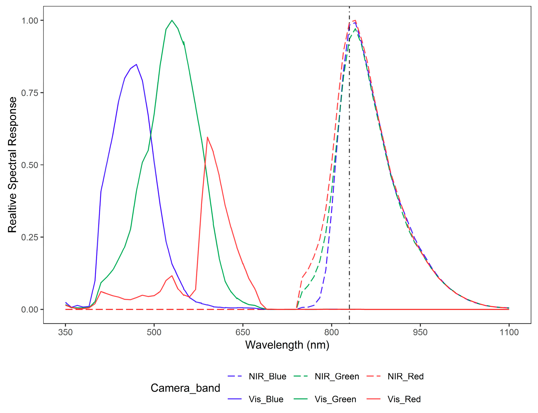
2.4.1. Relative Spectral Response

Relative Spectral Responses (RSR), Figure 2, of both cameras were determined using a double monochromator fitted with an integrating sphere, using the method described by Berra et al. [32]. The unmodified RGB camera shows greatest sensitivity in the green channel, as expected from a Bayer matrix colour filter array [32]. For the modified NIR camera, overall sensitivity was similar in all three bands that originally measured Red, Green and Blue waveband light. Whilst now mostly sensitive to NIR wavelength light, all channels show some sensitivity to light below 830 nm (i.e., sensitivity to radiation outside the NIR spectral range remained), indicating that the modified internal filter was not performing at 100% at 830 nm. The ‘Blue’ channel of the NIR-adapted camera displayed the least sensitivity to light below 830 nm, therefore was best suited for use as the NIR channel. The wavebands determined for each channel of the RGB and NIR channels are presented in

Table 3. Sony α5100 camera band sensitivities. Sensitivities were measured using a double monochromator fitted with an integrating sphere.

Model	Channel	Wavelength Range (nm)
“RGB” Camera	Red	580–660
	Green	420–610
	Blue	410–540
“NIR” Camera	NIR (blue channel)	800–900

.

2.4.2. RAW Conversion

Images were collected in RAW format before conversion to 16-bit Tagged Image File Format (TIFF) format using DCRAW 9.27 [36]. This was done using bilinear conversion algorithms and a dark current correction, to maintain original sensor DN measurements. The exact settings are presented in

Table 4. Details of DCRAW settings used to convert images from raw to Tagged Image File Format (TIFF).

DCRAW Command	Action
–v	Print verbose messages
–6	Write 16bit
–W	No automatic image brightening
–g 1 1	Apply unadjusted gamma curve
–T	Write Tiff format
–r 1 1 1 1	Set unadjusted white balance
–t 0	Do not rotate image
–q 0	Apply linear demosaicing
–o 0	Raw output colour space
–K darkimage.pgm	Apply dark image correction using file specified

. Dark current correction images for each camera were captured in complete darkness (i.e., lens cap on and lights turned off), and used for the DCRAW processing.

2.4.3. Exposure Corrections

To determine the relationships between DN and exposure settings (aperture and ISO), a series of images were collected of a Lambertian spectralon reflectance panel, set up indoors under constant illumination with a white incandescent bulb light. For each exposure setting (aperture, ISO and shutter speed), a series of images were captured under the settings full range (e.g., ISO100–ISO1000), whilst other settings remained fixed. As illumination remained constant; three image sets were produced, each modelling the influence of changing one exposure setting on image DNs.

Linear relationships between pixel DN and aperture and ISO were observed (Figure 3). From these relationships, the aperture correction factor (CF_app) was derived to normalise images captured under varied aperture to an aperture value of 1 (Equations (1) and (2)).

$$Imag{e}_{app}=\frac{Imag{e}_{RAW}}{C{F}_{app}}$$

(1)

where

$$C{F}_{app}=\frac{1}{{\left(fsto{p}_{image}\right)}^2}$$

(2)

where f-stop is the aperture value the image was captured with and Image_RAW is the DCRAW converted TIFF image and Image_app is the aperture corrected image.

For ISO, Equation (3) was used to normalise images to an ISO value of 100, the lowest and most commonly used setting on the cameras.

$$Imag{e}_{ISO}=\frac{Imag{e}_{app}}{\left(\frac{IS{O}_{image}}{100}\right)}$$

(3)

where ISO_image is the ISO setting used to capture the image; Image_app is the aperture corrected image; and Image_ISO is the ISO and aperture corrected image.

2.4.4. Vignetting Correction

An adapted version of the method outlined by LeLong et al. [16] was used in this study; such that camera, band and aperture-specific vignetting correction filters were generated for each data collection date. For each flight, the following steps were taken to produce vignetting filters:

• Images of matching camera, band and aperture settings were summed together and averaged.
• The radial vignetting profile of the averaged image was modelled using the median of evenly spaced concentric rings.
• A 2nd degree polynomial function interpolated the vignetting profile from the median of rings.
• The interpolation values were then divided by the minimum value to produce a multiplicative correction factor which brightened the corners.
• The concentric rings are given the value of the correction factor corresponding to its distance from the centre to produce the final vignetting filter (Figure 4 middle).

Unlike LeLong et al. [16], the vignetting filter was applied as a multiplicative filter rather than additive—this is in order to preserve the underlying patterns within the original images.

2.4.5. Cross Calibration Factor and Reflectance Calibration

Before converting image DNs to reflectance, it was necessary to cross calibrate the Tec5 downwelling sensor and the cameras. To do this, the empirical line method was used to retrieve the relationship between Tec5 irradiance measures and exposure and vignetting corrected image DN, over 5 Lambertian reference targets (Figure 5).

The camera and band specific calibration factors,

Table 5. Calibration equations for each of the four camera bands. Equations were derived from comparison of camera and Tec5 measurements of five reference targets.

Camera and Band	Calibration Equation
RGB-Blue	$0.0092\times \mathrm{DN}+0.00889$
RGB-Green	$0.00773\times \mathrm{DN}+0.00757$
RGB-Red	$0.0189\times \mathrm{DN}+0.00603$
NIR-Blue	$0.0249\times \mathrm{DN}-0.00706$

, were applied to individual images, before Equation (4) was used to convert images from DN to reflectance using time matched Tec5 irradiance measurements.

$$R_{b,t}=\frac{Imag{e}_{b,t}}{Tec5irradianc{e}_{b,t}}$$

(4)

where R_b,_t is the final reflectance image at time t and waveband b, Image_b,t is the single image captured at time t and band b, and Tec5 irradiance_b,t is the Tec5 irradiance measurement captured at the same time, t and convolved to the same band b as the image.

2.4.6. Orthomosaic Generation

Agisoft Photoscan (St. Petersburg, Russia) (1.4.3) [37] was used to process final imagery to orthomosaics, including automatic lens correction. For each date, two orthomosaics were generated, RGB and NIR. Agisoft processing settings,

Table 6. Processing settings for Agisoft Photoscan. The same settings were used for all Orthomosaics generated.

Processing Step	Setting
Align photos	High
Generate dense point cloud	Medium
Generate mesh	High
Generate orthomosaic	Disabled

, were kept consistent for all orthomosaics. In order to minimise the impact of geometric distortion and variation, the disabled blending mode was used to generate the orthomosaic [38]. This mode takes pixel data from the image whose view is closest to nadir. Orthomosaics were generated and exported at 1 cm Ground Sampling Distance (GSD).

NDVI orthomosaics were generated using Equation (5), before mean values for each plot in each camera band and NDVI were extracted using custom Python-based processing tools. As in Holman et al. [12], a 50 cm buffer was applied to each plot before extracting mean values in order to prevent the influence of the plot edge effect.

$$NDVI=\frac{R_{NIR}-R_r}{R_{NIR}+R_r}$$

(5)

where R_NIR is measured reflectance in the NIR band and R_r is measured reflectance in the red band.

2.5. Canopy Masking

To dissect green canopy from background variables, the Excess Green Red (ExGR) index was used (Equation (6)), with a threshold of > 0 to classify green vegetation [39,40]. Figure 6 shows an example of the produced mask, with reasonable agreement between visual green canopy and pixels classified as green by ExGR. The masks were used to extract mean plot NDVI of green pixels only.

$$ExGR=\left(2\times G-R-B\right)-(1.4\times R-G)$$

(6)

3. Results

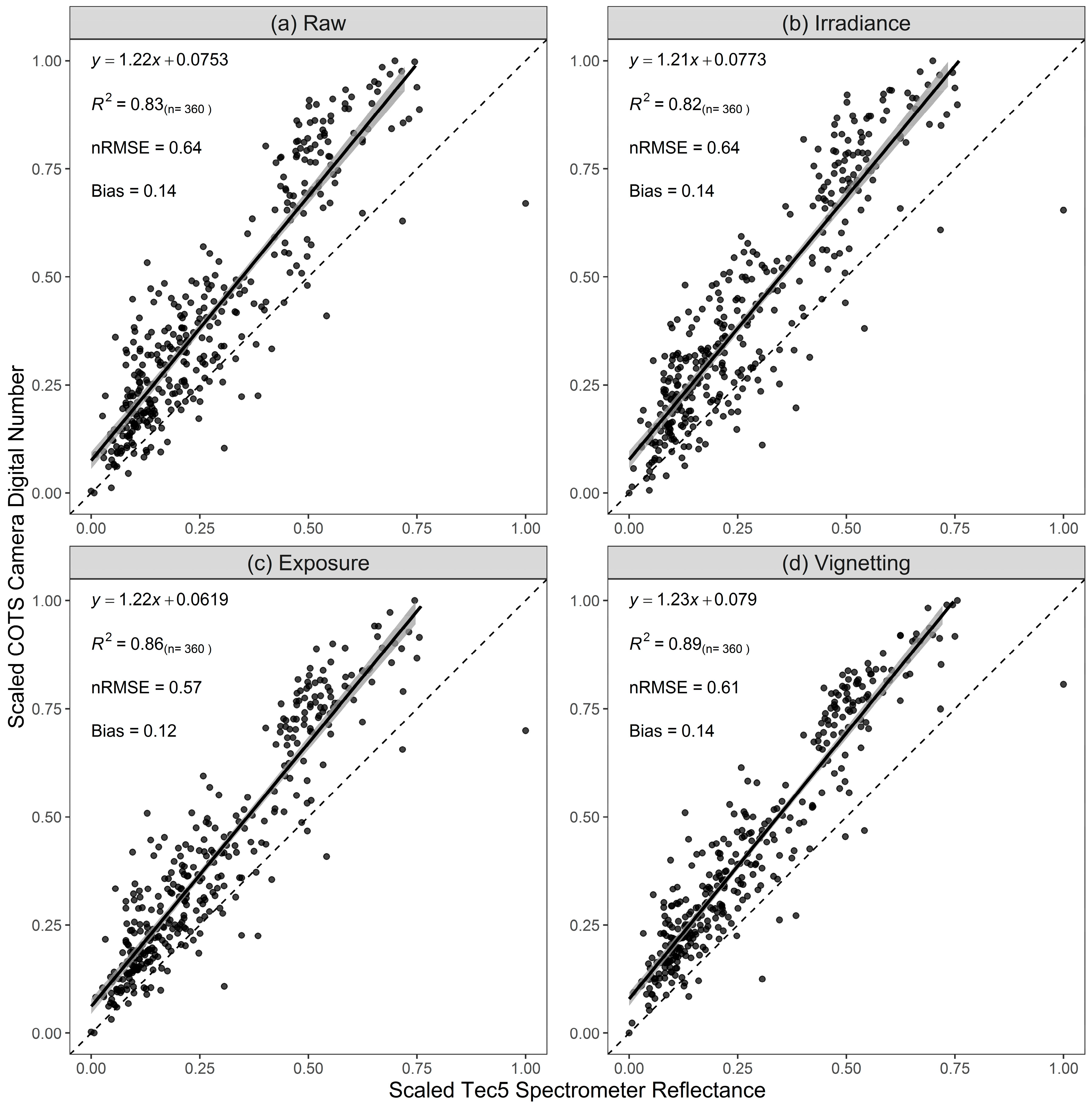
3.1. Validation of Calibrations

The influence of the calibration steps applied to COTS camera imagery on precision of results was first assessed. For a single date (21 June 2017), camera imagery was processed with corrections applied cumulatively to understand their influence on results. For clarity, extracted mean plot results for the red and NIR bands have been scaled to a range 0–1.

Red band results (Figure 7) show little impact on linear trend and intercept from correction steps, with consistent slopes around 1.2 and intercepts of 0.07. Correlations show improvement with addition of corrections, R²_RAW = 0.82 up to R²_Vignetting = 0.89, with camera-related exposure and vignetting offering the greatest gains. No meaningful effect on nRMSE and bias is gained from corrections.

For the NIR band (Figure 8), a more significant impact of correction steps is observed. Gains in both the linear fit and R² are achieved at each step, with vignetting indicating the most significant influence. Both nRMSE and bias decline in accuracy with the addition of correction steps.

The influence of corrections on NDVI, calculated from non-scaled data (Figure 9), indicates high precision (R² = 0.91) but poor accuracy (nRMSE = 0.85, Bias = −0.57) compared to the ground validation data. Addition of irradiance correction greatly improves accuracy, particularly nRMSE, bias and linear trend. Exposure corrections improve correlation, though drops in nRMSE and bias are also introduced. Finally, the addition of vignetting improves all statistics, indicating that the complete collection of calibration steps produces best results in terms of both accuracy and precision.

Further investigation of camera settings (Figure 10), via calculation on Exposure Value (Equation (7)), highlights how the cameras adjusted exposure independently during UAV flight. This independence explains the poor accuracy of NDVI from raw images, where variable camera settings (which can vary between the independent cameras used to gather RGB and NIR data) artificially altering the red to NIR ratio. Inclusion of the varying solar spectral irradiance data corrects this, improving the data consistency greatly; inclusion of exposure and vignetting corrections removes all influence of variable exposure settings, producing even higher accuracy data.

$$ExposureValu{e}_i=2\times lo{g}_2\left(f_i\right)-lo{g}_2\left(t_i\right)-lo{g}_2\left(IS{O}_i/100\right)$$

(7)

where f_i is the image aperture, t_i is the image shutter speed and ISO_i is the image ISO value.

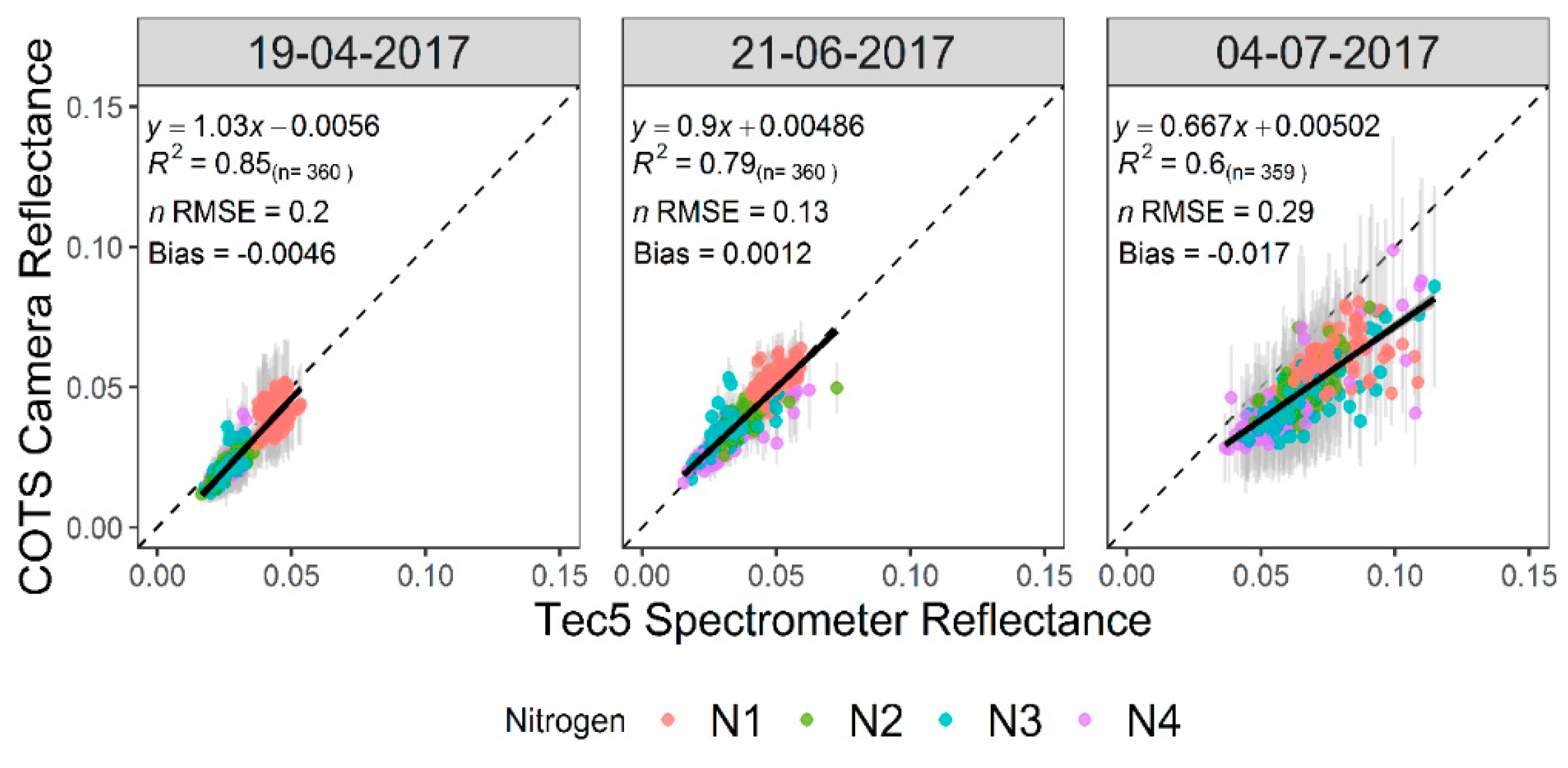
3.2. Accuracy Assessment of COTS Camera Reflectance

For three dates (19 April 2017, 21 June 2017, and 4 July 2017), the COTS camera-derived mean plot reflectance and calculated NDVI were assessed against Tec5 results. Results for the blue reflectance band (Figure 11) show good fit against the Tec5 in the first two dates (R² > 0.79), with slopes close to 1 and intercepts close to 0. Small nRMSE and biases also indicate good agreement with the spectrometer. Poorer results in all statistics in the last date (4 July 2017) show reduced agreement with Tec5 reflectance measurements. At this later date, onset of senescence will increase the variability in canopy reflectance both within and between plots, as seen by the increase in vertical error bars. This spatial non-uniformity of senescence onset is better measured by the UAV data as opposed to the spectrometer, leading to poorer statistics at this time point.

The green (Figure 12) and red bands (Figure 13) show very similar trends in accuracy to the blue band. Both bands show good fit (R² ≥ 0.84) and consistent small negative biases, indicating slight underestimation of reflectance from the cameras. The same trend between nitrogen treatments over time is also present, as well as the greater within-plot variation for the last date compared to the earlier two.

The NIR band (Figure 14) shows reduced fit in comparison to the visible bands (0.64 ≥ R² ≤ 0.7) and larger biases indicate lower accuracies achieved in the NIR band. In contrast to the visible bands, the NIR shows lowest accuracy in the first date before improving for the subsequent two dates. Trends between nitrogen treatments show that N1 treatments consistently have the lowest reflectance, indicating reduced vegetation in these plots, as expected. Standard deviations show the same increased variability in plot reflectance of the last date. Overall, the results of the NIR camera indicate lower sensitivity to higher canopy reflectance compared to the Tec5.

Accuracy assessments of calculated NDVI (Figure 15) show high correlations (R² ≥ 0.88) and low nRMSE. Additionally, biases indicating overall very good accuracy are achieved from the COTS cameras. Temporal accuracy shows a similar drop in accuracy for the final date, as seen in the visible bands, but overall good stability is achieved. The lower accuracy of the NIR band appears to not impact the accuracy of calculated NDVI.

Additional assessment compared results from the COTS cameras with the Parrot Sequoia (Figure 16), a commercially available multispectral imager whose data is processed using proprietary calibrations. Of the individual bands, green showed the strongest agreement between the two camera systems, with comparable R², nRMSE and bias. The red band indicated poorer accuracy achieved by the Sequoia, with large nRMSE, negative biases and poorer linear agreement with the Tec5. In the NIR band, both camera systems showed comparable accuracy levels and precision. NDVI results show greater accuracy achieved by the COTS cameras, with the Sequoia overestimating NDVI compared to the TEC5 (as indicated by positive bias). The similarity in results between the COTS cameras and Parrot Sequoia, particularly in the NIR waveband, suggests discrepancy between imaging and non-imaging spectral monitoring technologies.

3.3. Influence of Canopy on NDVI

The focus of this component of the study was to investigate the potential for high spatial resolution imagery to be used to dissect the influence of canopy cover on derived vegetation indices. For nine dates, the COTS camera imagery was calibrated, processed and NDVI calculated. For one date, 18 May 2017, significant shadowing impacted on the results of masking; as such, this date was removed from further processing. For the remaining eight dates, a subset of ten cultivars have been used. Examples of cropped NDVI orthomosaics for three dates highlight the temporal and spatial variation achieved from the COTS cameras (Figure 17).

Assessment of NDVI_unmasked (Figure 18a, top row) shows typical trends over time and between nitrogen treatments. All cultivars and treatment levels show a starting NDVI value around 0.4, increasing to a peak in late-May before dropping off at the end of the season. Comparison between nitrogen treatments shows clear differences between plots with (N2, N3 and N4) and without (N1) fertiliser application, with the N1 treatment showing lower maximum NDVI, despite similar initial NDVI values (~0.4). The drop in NDVI values at the end of the season is likely a result of senescence and the browning of crop canopy. Application of ExGR derived masks (Figure 18b, second row) to extract NDVI of green classified pixels only, produces new trends between treatments and over time. For all treatments, shallower temporal trends in NDVI are observed, with the N1 treatment displaying a close to horizontal trend with the peak in late-May no longer featuring. Comparing the difference between NDVI_unmasked and NDVI_ExGR (Figure 18c, third row) shows the greatest influence of masking occurs early season where % green pixel is lowest (Figure 18d, bottom row).

4. Discussion

This study has provided a quantitative assessment of commercial off the shelf (COTS) digital cameras for supporting the UAV-based remote sensing of field-based crop trials. COTS cameras provide very high spatial resolution imagery, potentially enabling the separation of canopy influences on vegetation indices from those of the background soil and thus making the derived information more relevant to crop health assessment and monitoring.

We have designed and tested a data processing workflow to radiometrically calibrate COTS camera imagery into reflectance units, in blue, green, red and NIR wavebands. Cameras were allowed to vary their exposure settings during flight, to cope with varying solar illumination conditions, whilst having a fixed shutter speed to avoid blurring from the UAV-motion. We find that our processing workflow can cope with this setup, and that the influence of the different pre-processing steps varies by band. In particular, the NIR band showed greater impact from vignetting corrections than the visible wavebands, agreeing with past studies which found that the modified internal filters used in NIR COTS cameras increase the impact of vignetting in images by up to 30% [16,25]. The influence of varied exposure settings as well as the success of the developed corrections was perhaps most clear during calculations of NDVI, because the separate visible and NIR COTS cameras used did not necessarily change their exposure settings in the same way at the same time, leading to artificial changes in derived NDVI. Even without corrections, good precision is observed in COTS camera calculated NDVI. However, NDVI values calculated from such raw camera data (or that calibrated into radiances rather than reflectances) are always significantly different to those derived from calibrated reflectances, and this difference is sensor specific [41]. Ultimately, this means VIs calculated from different sensors can only be intercompared in a fully meaningful way if calculated from calibrated reflectance measures.

Temporal consistency of the developed workflow was tested over three dates via comparison of COTS camera and Tec5 field-spectrometer-derived mean plot reflectance. Results showed good accuracy with NDVI results (R² ≥ 0.88, nRMSE ≤ 0.15) comparable to those achieved by other studies [25,42,43]. Consistency of results over this period indicates a good level of robustness in the developed methods for variable weather conditions both during and between data collection flights. Some variability occurred between time points in all bands and NDVI; likely a result of the UAV and Tec5 spectrometer obtaining measurements at different spatial resolutions [38] and datasets not being collected on the same date. Rossi et al. [44] demonstrated the impact of non-concurrent data collection when comparing different reflectance from different sensors, with a single day lag negatively impacting on correlation results. Variability in accuracy also occurred between bands, particularly for visible versus NIR, which was observed consistently over time. The same variations were also observed in the Parrot Sequoia results, as well as by Aasen and Bolten [38], who found that the varying field of views between cameras and spectrometers coupled with varying bidirectional reflectance factors in visible and NIR wavelengths impacted on correlations in the NIR band. Lack of influence of the NIR results on NDVI accuracy further indicates disparity between imaging and non-imaging measurement systems, as opposed to error in the NIR band. Investigation of this variability between bands and data sources should be a focus of future work.

Application of the very high resolution (GSD = 1 cm) reflectance imagery over time was used to investigate the impact of canopy cover and background soil on derived NDVI. Results of the unmasked NDVI presented temporal trends over a season in relation to differing nitrogen treatments and for different wheat cultivars. Masking of background soil pixels, via Excess Green Red, offered new insights into temporal NDVI trends in relation to canopy cover. Greatest differences between NDVI_unmasked and NDVI_ExGR (Figure 18d) occurred in the early season, where canopy cover is lowest [45], indicating that background soil and canopy cover can artificially influence measured vegetation indices. Isolation of the crop canopy for VI measurements should provide improved relationships between VI and traits of interest such as yield, canopy quality, senescence and canopy chlorophyll content [10,46], and therefore should be a focus of future studies.

5. Conclusions

This study has presented methods for radiometric calibration of commercial off the shelf digital camera imagery to reflectance for use in plant phenotyping. New calibrations for image exposure normalisation, combined with robust vignetting and irradiance corrections produced accurate reflectance and NDVI, comparable to a Parrot Sequoia multispectral camera and Tec5 ground spectrometer. The very high-resolution imagery obtained provided new insights into the influence of canopy cover and background soil on derived plot NDVI, especially in the early season. Future studies should look to incorporate additional UAV phenotyping methods such as 3D structure and thermal measurements to provide a more extensive low-cost phenotyping UAV-based system.

References

- Pask, A.J.D.; Pietragalla, J.; Mullan, D.M.; Reynolds, M.P. Physiological Breeding II: A Field Guide to Wheat Phenotyping; CIMMYT: Mexico City, Mexico, 2012. [Google Scholar]
- Khan, Z.; Chopin, J.; Cai, J.; Eichi, V.R.; Haefele, S.; Miklavcic, S.J. Quantitative Estimation of Wheat Phenotyping Traits Using Ground and Aerial Imagery. Remote Sens. 2018, 10, 950. [Google Scholar] [CrossRef]
- Kipp, S.; Mistele, B.; Baresel, P.; Schmidhalter, U. High-throughput phenotyping early plant vigour of winter wheat. Eur. J. Agron. 2014, 52, 271–278. [Google Scholar] [CrossRef]
- Cabrera-Bosquet, L.; Molero, G.; Stellacci, A.M.; Bort, J.; Nogues, S.; Araus, J.L. NDVI as a potential tool for predicting biomass, plant nitrogen content and growth in wheat genotypes subjected to different water and nitrogen conditions. Cereal Res. Commun. 2011, 39, 147–159. [Google Scholar] [CrossRef]
- Bendig, J.; Bolten, A.; Bennertz, S.; Broscheit, J.; Eichfuss, S.; Bareth, G. Estimating Biomass of Barley Using Crop Surface Models (CSMs) Derived from UAV-Based RGB Imaging. Remote Sens. 2014, 6, 10395–10412. [Google Scholar] [CrossRef]
- Muñoz-Huerta, R.F.; Guevara-Gonzalez, R.G.; Contreras-Medina, L.M.; Torres-Pacheco, I.; Prado-Olivarez, J.; Ocampo-Velazquez, R.V. A Review of Methods for Sensing the Nitrogen Status in Plants: Advantages, Disadvantages and Recent Advances. Sensors 2013, 13, 10823–10843. [Google Scholar] [CrossRef] [PubMed]
- Ali, M.; Montzka, C.; Stadler, A.; Menz, G.; Thonfeld, F.; Vereecken, H. Estimation and Validation of RapidEye-Based Time-Series of Leaf Area Index for Winter Wheat in the Rur Catchment (Germany). Remote Sens. 2015, 7, 2808–2831. [Google Scholar] [CrossRef]
- Zheng, G.; Moskal, L.M. Retrieving Leaf Area Index (LAI) Using Remote Sensing: Theories, Methods and Sensors. Sensors 2009, 9, 2719–2745. [Google Scholar] [CrossRef]
- Lopresti, M.F.; Di Bella, C.M.; Degioanni, A.J. Relationship between MODIS-NDVI data and wheat yield: A case study in Northern Buenos Aires province, Argentina. Inf. Process. Agric. 2015, 2, 73–84. [Google Scholar] [CrossRef]
- Jay, S.; Gorretta, N.; Morel, J.; Maupas, F.; Bendoula, R.; Rabatel, G.; Dutartre, D.; Comar, A.; Baret, F. Estimating leaf chlorophyll content in sugar beet canopies using millimeter- to centimeter-scale reflectance imagery. Remote Sens. Environ. 2017, 198, 173–186. [Google Scholar] [CrossRef]
- Duan, T.; Chapman, S.; Guo, Y.; Zheng, B. Dynamic monitoring of NDVI in wheat agronomy and breeding trials using an unmanned aerial vehicle. Field Crop. Res. 2017, 210, 71–80. [Google Scholar] [CrossRef]
- Holman, F.H.; Riche, A.B.; Michalski, A.; Castle, M.; Wooster, M.J.; Hawkesford, M.J. High Throughput Field Phenotyping of Wheat Plant Height and Growth Rate in Field Plot Trials Using UAV Based Remote Sensing. Remote Sens. 2016, 8, 1031. [Google Scholar] [CrossRef]
- Parrot SEQUOIA+|Parrot Store Official. Available online: https://www.parrot.com/business-solutions-uk/parrot-professional/parrot-sequoia (accessed on 8 April 2019).
- Young, N.E.; Anderson, R.S.; Chignell, S.M.; Vorster, A.G.; Lawrence, R.; Evangelista, P.H. A survival guide to Landsat preprocessing. Ecolgy 2017, 98, 920–932. [Google Scholar] [CrossRef] [PubMed]
- Lebourgeois, V.; Bégué, A.; Labbé, S.; Mallavan, B.; Prévot, L.; Roux, B. Can Commercial Digital Cameras Be Used as Multispectral Sensors? A Crop Monitoring Test. Sensors 2008, 8, 7300–7322. [Google Scholar] [CrossRef] [PubMed]
- Lelong, C.C.D.; Burger, P.; Jubelin, G.; Roux, B.; Labbé, S.; Baret, F. Assessment of Unmanned Aerial Vehicles Imagery for Quantitative Monitoring of Wheat Crop in Small Plots. Sensors 2008, 8, 3557–3585. [Google Scholar] [CrossRef] [PubMed]
- Mathews, A.J. A Practical UAV Remote Sensing Methodology to Generate Multispectral Orthophotos for Vineyards: Estimation of Spectral Reflectance Using Compact Digital Cameras. Int. J. Appl. Geospat. Res. 2015, 6, 65–87. [Google Scholar] [CrossRef]
- Gibson-Poole, S.; Humphris, S.; Toth, I.; Hamilton, A. Identification of the onset of disease within a potato crop using a UAV equipped with un-modified and modified commercial off-the-shelf digital cameras. Adv. Anim. Biosci. 2017, 8, 812–816. [Google Scholar] [CrossRef]
- Filippa, G.; Cremonese, E.; Migliavacca, M.; Galvagno, M.; Sonnentag, O.; Humphreys, E.; Hufkens, K.; Ryu, Y.; Verfaillie, J.; Di Cella, U.M.; et al. NDVI derived from near-infrared-enabled digital cameras: Applicability across different plant functional types. Agric. For. Meteorol. 2018, 249, 275–285. [Google Scholar] [CrossRef]
- Petach, A.R.; Toomey, M.; Aubrecht, D.M.; Richardson, A.D. Monitoring vegetation phenology using an infrared-enabled security camera. Agric. For. Meteorol. 2014, 195, 143–151. [Google Scholar] [CrossRef]
- Sakamoto, T.; Shibayama, M.; Kimura, A.; Takada, E. Assessment of digital camera-derived vegetation indices in quantitative monitoring of seasonal rice growth. ISPRS J. Photogramm. Remote Sens. 2011, 66, 872–882. [Google Scholar] [CrossRef]
- Sakamoto, T.; Gitelson, A.A.; Nguy-Robertson, A.L.; Arkebauer, T.J.; Wardlow, B.D.; Suyker, A.E.; Verma, S.B.; Shibayama, M. An alternative method using digital cameras for continuous monitoring of crop status. Agric. For. Meteorol. 2012, 154, 113–126. [Google Scholar] [CrossRef]
- Luo, Y.; El-Madany, T.S.; Filippa, G.; Ma, X.; Ahrens, B.; Carrara, A.; Gonzalez-Cascon, R.; Cremonese, E.; Galvagno, M.; Hammer, T.W.; et al. Using Near-Infrared-Enabled Digital Repeat Photography to Track Structural and Physiological Phenology in Mediterranean Tree-Grass Ecosystems. Remote Sens. 2018, 10, 1293. [Google Scholar] [CrossRef]
- Kelcey, J.; Lucieer, A. Sensor Correction of a 6-Band Multispectral Imaging Sensor for UAV Remote Sensing. Remote Sens. 2012, 4, 1462–1493. [Google Scholar] [CrossRef]
- Berra, E.F.; Gaulton, R.; Barr, S. Commercial Off-the-Shelf Digital Cameras on Unmanned Aerial Vehicles for Multitemporal Monitoring of Vegetation Reflectance and NDVI. IEEE Trans. Geosci. Remote Sens. 2017, 55, 4878–4886. [Google Scholar] [CrossRef]
- Smith, G.M.; Milton, E.J. The use of the empirical line method to calibrate remotely sensed data to reflectance. Int. J. Remote Sens. 1999, 20, 2653–2662. [Google Scholar] [CrossRef]
- Anderson, K.; Milton, E.J. Characterisation of the apparent reflectance of a concrete calibration surface over different time scales. In Proceedings of the Ninth International Symposium on Physical Measurements and Signatures in Remote Sensing (ISPMSRS), Beijing, China, 17–19 October 2005. [Google Scholar]
- Ritchie, G.L.; Sullivan, D.G.; Perry, C.D.; Hook, J.E.; Bednarz, C.W. Preparation of a Low-Cost Digital Camera System for Remote Sensing. Appl. Eng. Agric. 2008, 24, 885–894. [Google Scholar] [CrossRef]
- Hiscocks, P.D. Measuring Luminance with a Digital Camera. Available online: https://www.atecorp.com/atecorp/media/pdfs/data-sheets/Tektronix-J16_Application.pdf (accessed on 10 August 2017).
- Spreading Wings S900–Highly Portable, Powerful Aerial System for the Demanding Filmmaker. Available online: https://www.dji.com/uk/spreading-wings-s900 (accessed on 8 April 2019).
- Smart Camera|a5100 NFC & Wi-Fi Enabled Digital Camera|Sony UK. Available online: https://www.sony.co.uk/electronics/interchangeable-lens-cameras/ilce-5100-body-kit (accessed on 8 April 2019).
- Berra, E.; Gibson-Poole, S.; MacArthur, A.; Gaulton, R.; Hamilton, A. Estimation of the spectral sensitivity functions of un-modified and modified commercial off-the-shelf digital cameras to enable their use as a multispectral imaging system for UAVs. ISPRS–Int. Arch. Photogramm. Remote Sens. Spat. Inf. Sci. 2015, XL-1/W4, 207–214. [Google Scholar] [CrossRef]
- Geo 7X|Handhelds|Trimble Geospatial. Available online: https://geospatial.trimble.com/products-and-solutions/geo-7x (accessed on 8 April 2019).
- Customized Systems for HandySpec® Field|tec5. Available online: https://www.tec5.com/en/products/custom-solutions/handyspec-field (accessed on 8 April 2019).
- Professional Photogrammetry and Drone Mapping Software. Available online: https://www.pix4d.com/ (accessed on 10 April 2019).
- Decoding Raw Digital Photos in Linux. Available online: https://www.cybercom.net/~dcoffin/dcraw/ (accessed on 18 February 2019).
- Agisoft Agisoft PhotoScan User Manual Professional Edition, Version 1.2. Available online: http://www.agisoft.com/pdf/photoscan-pro_1_2_en.pdf (accessed on 24 August 2016).
- Aasen, H.; Bolten, A. Multi-temporal high-resolution imaging spectroscopy with hyperspectral 2D Imagers–from Theory to Application. Remote Sens. Environ. 2018, 205, 374–389. [Google Scholar] [CrossRef]
- Meyer, G.E.; Neto, J.C. Verification of color vegetation indices for automated crop imaging applications. Comput. Electron. Agric. 2008, 63, 282–293. [Google Scholar] [CrossRef]
- Sadeghi-Tehran, P.; Virlet, N.; Sabermanesh, K.; Hawkesford, M.J. Multi-feature machine learning model for automatic segmentation of green fractional vegetation cover for high-throughput field phenotyping. Plant Methods 2017, 13, 103. [Google Scholar] [CrossRef]
- Zhou, X.; Guan, H.; Xie, H.; Wilson, J.L. Analysis and optimization of NDVI definitions and areal fraction models in remote sensing of vegetation. Int. J. Remote Sens. 2009, 30, 721–751. [Google Scholar] [CrossRef]
- Hassan, M.A.; Yang, M.; Rasheed, A.; Jin, X.; Xia, X.; Xiao, Y.; He, Z. Time-Series Multispectral Indices from Unmanned Aerial Vehicle Imagery Reveal Senescence Rate in Bread Wheat. Remote Sens. 2018, 10, 809. [Google Scholar] [CrossRef]
- Hassan, M.A.; Yang, M.; Rasheed, A.; Yang, G.; Reynolds, M.; Xia, X.; Xiao, Y.; He, Z. A rapid monitoring of NDVI across the wheat growth cycle for grain yield prediction using a multi-spectral UAV platform. Plant Sci. 2019, 282, 95–103. [Google Scholar] [CrossRef] [PubMed]
- Rossi, M.; Niedrist, G.; Asam, S.; Tonon, G.; Tomelleri, E.; Zebisch, M. A Comparison of the Signal from Diverse Optical Sensors for Monitoring Alpine Grassland Dynamics. Remote Sens. 2019, 11, 296. [Google Scholar] [CrossRef]
- Agriculture and Horticulture Development Board (AHDB). Wheat Growth Guide; Agriculture and Horticulture Development Board (AHDB): Warwickshire, UK, 2015. [Google Scholar]
- Makanza, R.; Zaman-Allah, M.; Cairns, J.E.; Magorokosho, C.; Tarekegne, A.; Olsen, M.; Prasanna, B.M. High-Throughput Phenotyping of Canopy Cover and Senescence in Maize Field Trials Using Aerial Digital Canopy Imaging. Remote Sens. 2018, 10, 330. [Google Scholar] [CrossRef]