Abstract
The unprecedentedly strong 2016 Gyeongju and 2017 Pohang earthquakes on the Korean Peninsula aroused public concern regarding seismic hazards previously considered improbable. In this study, we investigated the effects of recent seismic activity close to the epicenters of both earthquakes in the heavy industrial complex of Ulsan. This was performed using Sentinel-1 InSAR time series data combined with on-site GPS observations and background GIS data. The interpretations revealed ongoing topographic deformation of a fault line and surrounding geological units of up to 15 mm/year. Postseismic migrations through the fault line, coupled with the two earthquakes, were not significant enough to pose an immediate threat to the industrial facilities or the residential area. However, according to InSAR time series analyses and geophysical modelling, strain from the independent migration trend of a fault line and eventual/temporal topographic changes caused by potential seismic friction could threaten precisely aligned industrial facilities, especially chemical pipelines. Therefore, we conducted probabilistic seismic hazard and stress change analyses over surrounding areas of industrial facilities employing modelled fault parameters based on InSAR observations. These demonstrate the potential of precise geodetic survey techniques for constant monitoring and risk assessment of heavy industrial complexes against seismic hazards by ongoing fault activities.
1. Introduction
Hazard assessment for past and future potential seismic activity is a significant topic in disaster management. The technical components for such tasks require highly sophisticated information synthetization for forecasting and monitoring of seismic energy sources and involves interpreting geological context and geospatial information on the target area where seismic deformation is imposed. In contrast to damage assessment of past earthquakes, which has frequently been the topic of remote sensing applications [1,2,3], the forecasting of future and on-going potential seismic hazards in specific regions of interest is highly challenging. This is because of technical barriers in identifying potential seismic sources and estimating their magnitude [4], and difficulties forecasting the correlation with socio-economic backgrounds. Therefore, it is necessary to introduce technological advances in remote sensing to estimate the potential seismic sources from minor clues and quantitative analyses based on the extracted geophysical information from in-orbital sensors such as Interferometric Synthetic Aperture Radar (InSAR) for precise geodetic survey. Motivated by such ideas, we tackled a range of technical issues in assessing potential seismic hazards, particularly over heavy industrial hubs in which significant threats are heavily imposed owing to the secondary effects of earthquakes.
Korea, where the target area of this study is located, has previously been considered relatively safe from seismic hazards owing to an absence of major active tectonics. However, two recent earthquakes, the 2016 Gyeongju (magnitude 5.8, depth of epicenter 15.2 km) event [5,6,7] and the 2017 Pohang (magnitude 5.4, depth of epicenter 6.9 km) earthquake event [8,9], have aroused national concern about the safety of residential, industrial, and social infrastructure. Before the 1990s, Korea did not have any regulations on earthquake resistant construction design; given the growing population and development of industry and infrastructure, this could trigger socio-economically disastrous events, the so-called domino effect [10]. The south-eastern part of the Korean Peninsula is the densest industrial hub equipped with chemical, heavy machinery, and atomic power planets; incidentally, in close proximity with the epicenters of the two recent earthquakes. Although the magnitude of two earthquakes were below generally accepted critical values (magnitude 6.5 to 7.0) for significant structural damage, the city of Ulsan fell under public scrutiny because of its high concentration of transportation networks for chemical agents, heavy production facilities, and high population density. There is concern for the safety of the city from coseismic, postseismic, and even preseismic surface motion, based on historical cases [11,12,13,14]. A major concern is the vulnerability of industrial pipelines filled with toxic and combustible liquid materials [15,16]; note that earthquakes are responsible for 5% of all incidents of poisonous chemical material exposure [17,18]. In addition, direct damage from earthquakes include the impacts of liquefaction, which could result in serious damage to sensitive industrial facilities. Hence, a series of studies are being conducted to assist with the preemptive design of facilities and postinvestigation methods [19,20,21].
In the case of Ulsan, in addition to government bodies initiating a sequence of ground surveys for safety checks over major facilities, a geodetic campaign employing space borne assets and a GPS network was proposed to address the complexity and extent of the target area. We conducted Interferometry Synthetic Aperture Radar (InSAR) observations together with GPS/GIS data analysis and geophysical modelling to assess the vulnerability of Ulsan to surface deformation, and focused on the relationship between recent (2015–2018) and future potential seismic activities and the plausible risks of industrial infrastructure. InSAR techniques have been employed to investigate the effects of seismic activity and surface deformation in a large number of studies; it is a well-demonstrated method for determining potential hazards, particularly earthquakes [22,23,24], and for evaluating the associated damage [25,26,27]. However, our aim was to investigate the effects of relatively minor earthquakes and to monitor the potential damage from accumulated subtle strain over highly sensitive infrastructure facilities. Thus, InSAR time series analysis was employed as error components of InSAR processing need to be suppressed and the outcomes was carefully interpreted together with GIS and geophysical modelling. Technically, this study focused the feasibility of InSAR remote sensing approaches for the safety surveillance of industrial infrastructure, which requires high precision measurements, as well as the investigation of subtle pre/postseismic surface deformation over the target area. Thus, it differed from past studies that have used geophysical data to investigate obvious coseismic raptures using multipass InSAR observations. The consequent technical challenges involved in mining the potential seismic risk elements from weak/continuous deformations were overcome via spatial/temporal interpolation of InSAR time series analyses and 3D decompositions. The extracted information was feed forwarded to geophysical models and again synthesized with probabilistic seismic hazard analysis (PSHA) [28] to extract corresponding risk maps.
The associated target area context and data sets are described in Section 2. The processing methodologies for InSAR and auxiliary data sets with their outcomes are given in Section 3 and Section 4, respectively. A discussion on the detected deformation and the geophysical inversion modelling work validating the DInSAR observations is presented in Section 5.
2. Context of Target Area
The city of Ulsan is located in the south-east of the Korean Peninsula. It has undergone rapid industrial development since 1960 as the central hub for heavy/chemical industries such as the automobile, shipbuilding, metal, petrochemistry, and chemical component industries. Two major contextual characteristics of Ulsan (Figure 1) are that: (1) it is connected to the fault lines that encompass the two epicenters of recent earthquakes; and (2) a portion of the central city and the industrial components were built on reclaimed land or sedimentary valleys corresponding to an active fault, called the Ulsan fault line. Figure 1 shows the structural geology of Ulsan. The Yangsan fault, a major 170 km fault line with a strike-slip form, is considered the primary contributor to the 2016 Gyeongju earthquake that hit the eastern section of Ulsan. Reclaimed land in the south of Ulsan, where the industrial facilities are mainly located, lies over the Ulsan fault (160 degree strike angle from north, 50 km length), the left branch of the Yangsan fault. Although debate remains about the status of both faults, it has been more or less confirmed that both are active [29,30]. Kyung [31] estimated slip rates of 0.1–0.04 m/ka and 0.2–0.06 m/ka for the Yangsan and Ulsan faults, respectively. Choi et al. [32] proposed a 0.18–0.28 mm/year slip rate for the branches of the Ulsan fault. In general, the Ulsan fault is considered more active than the Yangsan fault and will likely trigger future seismic activity.
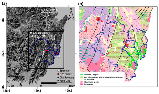
Figure 1.
Location and geological context of the target area. The epicenters of two major earthquakes, the involved faults lines, and two GPS stations (ULSN and WOLS) around the target area are described in terms of (a) the target area topography and involved contexts and (b) its geological context together with the locations of the industrial complex.
The Ulsan Petrochemical Complex (UPC) is equipped with ~20–50-year-old underground pipeline, and these have become a major concern for city and national government bodies in terms of chemical leakage risks. Although safety diagnosis and a remodeling support project have been actively underway since the two earthquakes occurred, the large target area (≈935 km2) would make a comprehensive remodeling of networks impossible. Underground buried pipelines in the UPC are up to 1150 km long, and include a 568 km chemical materials transportation line, 425 km of gas pipes, and 143 km of oil pipelines.
Central Ulsan lies on soft ground, mainly reclamation land that is encircled by industrial facilities and houses a population of 200,000 (Figure 1b). After being subject to physical damage from the two earthquakes, and subsequent sinkhole development in recent years, the city government has investigated liquefaction over the soft reclaimed ground. As the area is built over tideland with a rock layer lying 10 to 50 m underground, the central city area and industrial parks were deemed to be at high risk for surface deformation. Although imminent risks of ground deformations have not been identified, such risks demand prompt geodetic surveys and consequent interpretation together with geophysical modelling and GIS analyses.
3. Data Sets and Methods
As a powerful tool that efficiently assesses potential natural hazards involving ground deformation, InSAR has been widely employed for seismic activity monitoring [33,34,35], land subsidence [35,36], and landslides [37,38,39]. In theory, InSAR is capable of tracing surface deformation up to a few millimeters in ideal error free conditions [40]; however, phase delay components together with externally induced errors such as base DEM and orbital information pose obstacles for precise measurement of surface deformation [41]; thus, the compensation of Atmospheric Phase Screen (APS) is significantly important to ensure precise InSAR measurements. The precision required for our study is a maximum of few tens of millimeters because the deformation over the target area is not a consequence of major earthquake or well confined ground subsidence. To correctly assess the hazards in the target area, we employed rigorous InSAR time series analyses and fused the outcomes with GPS, geophysical modelling, and GIS data.
3.1. Data Set Description
There are InSAR images over the target area, including three InSAR pairs L band ALOS PALSAR-2, a few X band Terra X SAR, and COSMO Skymed only around the Ulsan city area. L band PALSAR-2 is more coherent over all landcover types and X band SARs provide optimized resolution to observe the central city area. However, none of them, except Sentinel-1 SAR, have suitable temporal coverages to investigate two separate earthquakes with a time series analysis approach. The optimal data set for this study was Sentinel-1 SAR imagery, which is freely available on the Sentinel data hub. It is acquired by two SAR-satellite constellations that are composed of Sentinel 1A, which was launched in April 2015, and Sentinel 1B, which was launched in April 2016. The characteristics of C band wavelength and Interferometric Wide-swath mode (IW) operation with Terrain Observation and Progressive Scans SAR (TOPSAR) imaging allow for more precise monitoring of the target area with relatively minor ionospheric errors and wide coverage (Swath > 250 km), together with moderate spatial resolution (20 m in azimuth and a 4 m range) [42]. The biggest merit of the Sentinel-1 constellation is its short revisiting time (14 days); thus, the image graph for time series analysis consisting of 60 ascending modes and 86 descending modes can be readily composed for a three-year time period as shown in Figure 2. The other image characteristics of Sentinel-1 imagery are summarized in Table 1. InSAR observations covering the temporal coverage to monitor the long-term deformation trends of pre/co/postseismic phases with sufficient spatial resolution and extent was found to be feasible throughout multiple Sentinel-1 image sets.
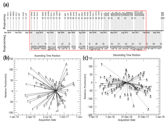
Figure 2.
Acquisition time (a) and connection graphs of employed Sentinel-1 InSAR pairs (b,c). In total, 60 ascending and 86 descending images were employed for time series analysis. Note: the red box in (a) represents the target period of decomposition.

Table 1.
Characteristics of employed Sentinel-1 images.
3.2. Permanent Scatterers Analyses of InSAR Pairs
In order to detect subtle ground deformation over the target area, a number of error components of the DInSAR phase have to be dealt with using proper error suppression techniques. The main error source is the electromagnetic phase delay by troposphere water vapor turbulence, (i.e., the wet delay component). The stratified phase delay, called the dry delay component, is not significant owing to the relatively low topographic relief of the target area.
The target area is located on the eastern coastal line and experiences large seasonal precipitation variations (seven times higher in summer than winter). This phenomenon is attributed to orographic effects, where the seasonal unequaled water vapor distribution dominates in the eastern coastal area of the Korean Peninsula. These effects are caused by the topographic profile and by water vapor from the eastern sea, and they frequently mislead the interpretation of InSAR processing [43] and need to be regulated. In InSAR time series analysis, stacking multiple interferograms helps estimate and reduce errors from water vapor and from an inaccurate base DEM. The InSAR time series technique was largely classified by Permanent Scatterers (PS) by Ferretti et al. [44,45] and Small Baseline Subsets (SBAS) by Berardino et al. [46] according to the InSAR pair connection methods (i.e., 1 to 1 connection in PS and many to many in SBAS). The algorithmic improvements of time series analysis mainly aim for the densification of reliable scatterers and have proven capabilities [47]. However, according to a preliminary PS InSAR analysis, it appeared that the temporal and spatial baseline conditions between SAR images in this study were adequate to address those technical challenges with an ordinary PS algorithm, as shown in Figure 2. It was also observed that the density of extracted scatterers was sufficient for further interpretation (see Figure 3). This is because the densified artificial structures of the target area are optimal for producing stable scatterers, which are essential for the success of PS algorithms.
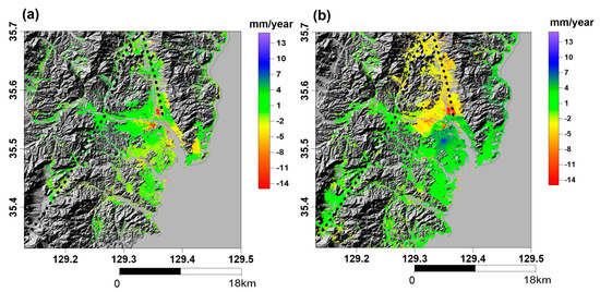
Figure 3.
(a) Line of sight (LOS) displacements by ascending mode InSAR time series analysis during November 2014 to July 2018 and (b) descending mode InSAR time series analysis during May 2015 to June 2018. Note the locations of the Yangsan and Ulsan fault lines, represented as dotted lines.
The error terms that need to be suppressed by PS algorithms can be expressed as follows:
where ΦE is the phase difference by whole error factors, Φa is the phase difference by atmospheric error terms, Φo is the phase difference by inaccurate orbital information, Φt is the phase difference by inaccurate DEM, Φn is the phase noise, Φtropospheric is the phase difference by tropospheric components, and Φionospheric is the phase difference by delay in the ionosphere.
Because the target has a relatively flat topography, which is ideal for successful inversion of PS processing, it was theorized that PS algorithms could effectively suppress major error components. However, the temporal gap between the image acquisitions and the construction time of the base DEM, almost 20 years in the case of SRTM DEM usage, can pose complications for the application of PS algorithms over heavily rebuilt topography (e.g., that of the target area). Therefore, we employed the ALOS PRISM DEM, which was extracted from a 2005–2010 stereo mission [48], as the base DEM of PS processing. In addition to improving temporal coverage, the ALOS PRISM DEM has better vertical accuracy over the central city area owing to its intrinsic characteristics of 2.5 m resolution stereo matching compared to interferogram processing with a 15 m resolution in the SRTM resolution. We first tested the vertical accuracy of ALOS PRISM DEM using geodetic survey points over target areas. As the survey points were located in stable crossovers of road networks and bare field, they were expected to show the intrinsic geodetic control accuracy of both DEMs over the test area. The data in Table 2 showed that the accuracy of ALSO PRISM DEM is far better than that of the SRTM DEM 1 arc sec product. The test time series analyses using ALOS PRISM and SRTM DEM demonstrated highly similar deformation patterns, which indicate the effectiveness of PS error correction algorithms. However, the processing outcome by PS with ALOS PRISM DEM produced slightly better phase coherences in every InSAR pair combination (0.286 of SRTM DEM processing and 0.291 of PRISM DEM processing). The improvements in phase coherence reflect better coregistrations based on initial positioning of conjugated points employing the 3D coordinate of base DEM. Therefore, it was proposed that PS processing employing an ALOS PRISM base DEM and 60 to 86 Sentinel-1 SAR images in ascending and descending mode, respectively, produced enough quality outcomes to trace potential surface migration. On the other hand, the quality of PS InSAR processing was again assessed by intercomparison with GPS data in Section 4 and the possibility of error remnant, especially with orbital error component, is further discussed in Section 5
Table 2.
Intercomparison between survey control points and Shuttle Radar Topography Mission (SRTM) and Advanced Land Observing Satellite (ALOS) Panchromatic Remote-sensing Instrument for Stereo Mapping (PRISM) DEM. Eleven survey control points were employed for the assessment.
3.3. GPS Data Set and Processing
In this study, the datasets from two GPS continuous observation stations (Figure 1a) were employed for the verification of InSAR displacements. The WOLS station, operated by the National Geographic Information Institute (NGII), is located on stable ground, whereas the ULSN station is located on the roof of a building, which makes data less reliable for validation of deformation data owing to the thermal expansion of the building roof. The GPS processing period covered 2.5 years, from 1 January 2016 to 30 June 2018, and was conducted using relative positioning (RP) employing Bernese 5.2 S/W [49] for the extraction of locations and time series analysis of the station referencing. For precise position estimation, the International Terrestrial Reference Frame (ITRF) 2014 was applied and the GPS satellite trajectory was then postprocessed using ephemeris provided by the Center for Orbit Determination in Europe (CODE). It should be noted that the ITRF 2014 coordinates of stations were extracted from nine International GNSS service (IGS) Stations in China, Japan, Russia, and Mongolia. Then, the coordinates were again adjusted using the minimum constraint method, considering Helmert conversion elements and the stability of reference stations by the RP module of Bernese S/W. The parameters and models used to remove various GPS errors are given in Table 3. To segregate the background and seasonal migration of GPS observations, we conducted additional operations on GPS migrations. Find Outliers and Discontinuities In Time Series (FODITS) module [50] in the Bernese GPS Software was employed to eradicate outliers, discontinuities, and one or more linear velocities from GPS observations. For comparison, the seasonal components were interpolated using sinusoidal approximation [51], which can be expressed as follows:
where Y is coordinate displacement, A is amplitude, ω is frequency, t is observation time, and ϕ is phase. As the outcomes from both methods fitted each other well, the seasonal components in the GPS signal were considered to be effectively removed.
Table 3.
Processing method/parameters of GPS data.
4. Results
4.1. Surface Deformation by PS Analysis
Figure 3 shows the Line of Sight (LOS) displacements extracted via the PS time series analysis in the target area. The multiple reference points by the analyses of phase angles of each interferograms were generated on the stable ground surfaces. Therefore, deformation values in booth ascending and descending analyses were fitted on the same spatial and temporal reference frames to be feed forwarded to decomposition. The time series displays of LOS surface deformations (ascending mode in Figure 4 and descending mode in Figure 5) demonstrate that the deformation patterns along geological/landcover units were consistent overall. However, there were strong discrepancies between the ascending and descending mode observations in a few geological units, particularly along the Ulsan fault line. This implies that surface migration along the Ulsan fault was typically governed by horizontal translation. As the accuracy and effectiveness of PS analysis in eradicating the error components needed to be investigated, we conducted an intercomparison test between the GPS and InSAR deformations.
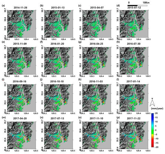
Figure 4.
Temporal migration of LOS deformation in ascending mode during the 2014–2018 period, where (i) and (p) are the coseismic displacements of two earthquakes. The referencing time of deformation is 26 November 2014. Note the localized strong deformation in the eastern city area and the locations of two faults, represented as black lines.

Figure 5.
Temporal migration of LOS deformation in descending mode during the 2015–2018 period. The referencing time of deformation is 25 May 2015. Deformation along the Ulsan fault was apparent first.
4.2. Migration Vector Decomposition and Intercomparison with GPS Data
Line of sight (LOS) deformations only showed the projected displacement in the employed sensor directions. Thus, it was necessary to decompose InSAR displacement to analyze surface deformation quantitatively, involving geological contexts. The decomposition of the horizontal and vertical displacement vectors from the ascending–descending time series combinations was performed as follows. First, the descending time series displacement maps from corresponding InSAR pairs (refer to the red boxed portions in Figure 2a) were interpolated spatially to increase observation density and temporally to fit the referencing time of deformations of two time series observations. They were then rearranged into 54 interpolated displacement maps according to the acquisition times of the ascending mode InSAR pairs. The temporal displacement values for specific locations were interpolated using a least squares quadratic equation fit with a 2nd order polynomial function, and a spatial adaptive filter was applied over newly arranged deformations. For the 54 ascending and interpolated descending displacement pairs which now have better observation densities and the same reference time of deformation measurement, i.e., 2015/05/25, vector decomposition was conducted as per the method described in Fialko et al. [35].
where dispLOSasc is ascending mode displacement, dispLOSdisp is descending mode displacement, dispH, and dispV are horizontal and vertical displacements, respectively, and sinθasc and sinθdesc are the look angles of the ascending and descending modes, respectively.
The horizontal displacement extracted by decomposition consisted of two components that are related as follows:
where dispNS is the N–S directional displacement, dispEW is the E–W directional displacement, and φ is the heading angle of the satellite. As the heading angles of the satellite can be approximated to 0° and 180°, the contribution of E–W displacement to horizontal displacement is far more significant (by about three times in Sentinel-1 image acquisition geometry) than that of N–S displacement. In the present study, it was not possible to decompose the E–W and N–S displacements because we only had two observations.
Horizontal and vertical displacements in both the ascending and descending total cumulative/time series observations are given in Figure 6. We identified strong deformation in both the vertical and horizontal directions along the Ulsan fault (P1 and P3 in Figure 6) and found stabilities along the Yangsan fault (P6 in Figure 6). Those outcomes were used to analyze the geological context of the industrial facilities, which involved risk factors, together with geophysical models (see Section 5).
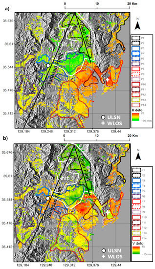
Figure 6.
Horizontal (a) and vertical (b) displacement by decomposition. Total cumulative values during in June 2015 to January 2018 and the temporal evolutions in major deformation units (see Table 4 for details). Note the locations of P1 and P3 and the Ulsan fault line along with Unit 1.
In order to validate InSAR observations and to extract more information, a comparison with GPS data from the WOLS and ULSN stations was conducted. The LOS deformations around the P3 and P10 areas (Figure 6), which are defined by geological units and a specific deformation pattern (see Section 5 for details), were compared to the nearest WOLS and ULSN GPS data. It should be noted that (1) the GPS measurements were corrected for background and seasonal trend, as explained in Section 3.3; (2) GPS data were converted into LOS values using Equations (7) and (8). Although there are some slope differences between GPS and InSAR deformations, concurrent migration trends in the ascending and descending modes were obvious in both GPS and InSAR (Figure 7). Considering that GPS migration is mostly in the E–W direction and that InSAR observations are far more sensitive in E–W rather than N–S directional migration, we concluded that migrations along corresponding areas are mostly governed by E–W directional deformation. In addition, our proposed PS algorithms to suppress error terms worked well based on the trends of GPS and InSAR observations, which demonstrated good agreement, except for some differences in migration speeds presented in Figure 7b,d. It is worth noting that the entire southern Korean peninsula has a peculiar drift to the eastern side of up to few tens of mm/year [51,52] since 2010 Tohoku earthquake. Therefore, the migration slope difference on WOLS (Figure 7b,d) can be naturally explained by the referencing differences between InSAR which is referenced on the local domain of this study and GPS, which is referenced from nine International GNSS service (IGS) Stations and consequently influenced by the migration of the southern Korean peninsula. We found that 25 mm/year is the optimal drift value to minimize the slope difference between GPS and InSAR measurements.
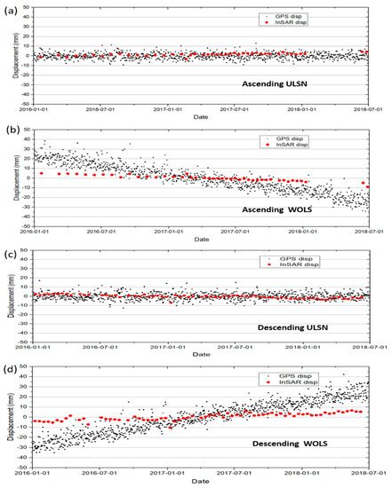
Figure 7.
Ascending mode LOS deformations compared to ULSN (a) and WOLS GPS data (b) and descending mode LOS deformations compared to ULSN (c) and WOLS GPS data (d) are presented. Total cumulative values during January 2016 to July 2018 were analyzed. All GPS and InSAR observations are referenced to 01 March 2017 for seasonal variation processing. Note the seasonal correction in WOLS is only applied to Up-Down GPS observation as seasonal correction on the E–W GPS component produced a highly scattered pattern. The systematic migration speed differences in (b) and (d) were explained by the referencing issue and peculiar drift of southern Korean peninsula.
5. Discussion
5.1. Interpretation of Deformations and Geophysical Modelling
In order to quantitatively interpret the deformation at Ulsan, we defined a total of 14 units over the major InSAR observations considering geological contexts and the deformation characteristics represented in Figure 6 and Table 4. The first possible assumption on the categorized deformation patterns was that the main deformation in the Ulsan area was induced by the Ulsan fault and its interactions with the surrounding geological units. Together with the analyses of ongoing deformations, we investigated the influences of the two recent major earthquakes using the observations of horizontal and vertical deformation time series shown in Figure 8 and Figure 9. It is clear that none of the units showed a noticeable footprint from the two earthquakes. Thus, we concluded that the 2016 and 2017 earthquakes were not coupled with the deformation sources in the Ulsan local area. Note that a significant deformation change occurred around February to March 2017, which we surmise to be a PS time series processing blunder because we did not identify any seismic activity or significant water vapor distribution as an error source. The interpretation is as follows. The southern Korean peninsula in the 2017 spring season had one of the worst droughts. The record in our WOLS, ULSN GPS Precipitation Water Vapor (PWV) also showed 1–2 mm values in high contrast to the mean spring PWV 10–12 mm in 2016 and 2017 as well as 70–80 mm for the summer season PWV. As the master image of the ascending time series was assigned to February 2017, the tropospheric phase delays around the InSAR image pairs of winter to spring 2017 are considerable low compared to the other pairs. Therefore, InSAR APS in the winter to spring 2017 term behaved like the nonsteady component proposed by Hopper et al. [53]; thus, it is difficult to address, especially with the linear APS modelling that is normally implemented [54] in PS routines, considering that the tropospheric error by such extreme change on the temporal weather condition might cause different APS patterns from topography correlated components which is better studied [55]. Fortunately, it did not impair the overall quality of the DInSAR analysis deformation because the blunder only constituted a small portion of the time series observation. The solution is to introduce presuppression of APS via an atmospheric model combined with time series analyses as shown in Jung et al. [56] and Li et al. [57], if high-resolution weather modelling is feasible.
Table 4.
Categorized deformation units and their characteristics.
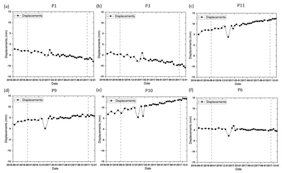
Figure 8.
Time series observations of horizontal displacements in unit (a) P1, (b) P3, (c) P11, (d) P9, (e) P10, and (f) P6. Two vertical dotted lines represent the 2016 Gyeounju (12 September) and 2017 Pohang (15 November) earthquakes. No units show a significant change during the coseismic period. The sudden change February to March 2017 might originate from the coinciding of the master image section and extreme APS value.
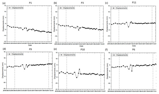
Figure 9.
Time series observations of vertical displacements in unit (a) P1, (b) P3, (c) P11, (d) P9, (e) P10, and (f) P6. Two vertical dotted lines represent the 2016 Gyeounju (12 September) and 2017 Pohang (15 November) earthquakes.
The other issue to be addressed is whether the observed defamation originated by genuine fault migrations or the remnants of InSAR processing errors. It should be noted that the Ulsan fault has been proven to be active by multiple geological surveys [30,32], compared to the Yangsan fault represented in Unit 6. Thus, the only problem is confirmation of the Ulsan fault line’s activeness up to 20 mm/year as identified by InSAR time series analysis. The possibility that the InSAR phase difference around fault lines (P1 and P3) originated from error elements was refuted as follows. First, the error elements by base DEM and/or atmospheric effects should be removed by PS time series algorithms. Although there is a minor effect of the unresolved error components, it can’t produce the deformation patterns in both ascending and descending modes that fit exactly with our active Ulsan fault scenario. Although PS time series algorithms cannot effectively address orbital components, a candidate of the false surface deformation source, as stated in some studies [58,59], the orbital error is usually represented by a tilt shape [60,61] in InSAR time series output. Therefore, it does not fit with the observed deformation pattern around the Ulsan fault line. The concurrent InSAR observation by ascending and descending modes is very useful in inferring orbital error components because the orbital error component cannot produce proper deformation patterns that fit with the modeled deformation source in two observation modes, simultaneously. Thus, our results in ascending and descending observations fully eradicated the possibility of error terms around the Ulsan fault.
The task to identify the deformation source from the InSAR observations can be accomplished through modelling of fault perpendicular deformation on certain constraints such as full strike slip fault geometry [62,63,64]. However, in the case of the Ulsan fault, any specific constraint on fault migrations is highly unlikely as observed in precedent studies on ground surveys [29,30,31,52]. In these circumstances, we performed a geophysical inversion, employing the Geodetic Bayesian Inversion Software (GBIS) [65] to define more clearly the deformation source and its contributions. This software is capable of deformation source parameter inversion using Markov-chain Monte Carlo methods [66] and the Metropolis–Hastings algorithm [67] even with InSAR observations in a complicated scenario [68]. We assigned the initial parameters of the fault line sets (Table 5) based on the known geometry of the Ulsan fault, and considered two plausible scenarios: (1) the Ulsan fault and its interaction with the surrounding soft ground units is responsible for the deformation pattern in the target area (i.e., the single fault model); and (2) full deformation is induced by the interaction between multiple faults, and thus the fault system could produce a localized deformation in the Ulsan central city area (i.e., the multifault model).
Table 5.
Initial parameter settings for GBIS modelling and modelled values.
The multifault line model, consisting of the Ulsan fault and the fault lines directly crossing Ulsan city area, is less feasible because it unlikely that there are unknown fault lines in the Ulsan central city area, where highly intensive survey works have been constantly conducted for several decades. However, since the multifault model based on Ulsan fault line segmentation has been proposed by recent studies [69] is remains feasible; therefore, we established fault segments along the Ulsan fault line for the multifault model scenario. For the multifault models, GBIS automatically developed multifault line parameters from a set of initial fault parameters during iterations. Quadtree subsampling of ascending and interpolated descending deformations via the PS time series and their subsequent forward modelling using the GBIS routine yielded the fault line parameters (Table 5). The single fault model produced more adequate results than the multiple fault model as shown in the fitness values of models, although neither fully addressed the local mismatches between models and observations. In particular, the enormously large slip rates and abrupt change of slip direction in the multifault simulation (Table 5) raises doubt in the reliability of multifault segmentation models. Thus, it is reasonable to propose that tectonic deformation was mostly driven by migration of the Ulsan fault. The error residuals of the single fault model can be interpreted as the interaction of minor tectonic lineaments or partial difference of modulus values over sedimentary/reclaimed plains, which cannot be modelled in contemporary inversion schemes.
5.2. Risk Assessments
The modelled parameters of the Ulsan faults were again employed for quantitative risk scenarios on the industrial parks centered around UPC based on two different approaches, i.e., Coulomb Failure Function (CFF) estimation and PSHA methods.
At first, to quantitatively evaluate the future fault failure risk in the target zones, we modelled the coulomb stress on the lineament for the Ulsan central city area and for the industrial parks (Figure 10). Since the stress during earthquake is transferred by propagation along surrounding faults and segments [70,71] as well as regional dispatch, CFF estimation on the lineament close to the target area implies the risks of the time of future potential earthquakes. From our observations, we now know there is a discontinuity between the Ulsan fault units and the deformation units of the central city area, which may represent the boundary of sedimentary plains. However, we also propose the existences of a second boundary between sedimentary plains and reclaimed grounds where the industrial parks are mostly located. We defined two lineaments (L1 and L2, represented as boundaries 1 and 2 in Figure 10) along with those boundaries between Unit 2 and 4 and calculated the CFF employing the modelled Ulsan fault line parameters. As demonstrated in Figure 10, it was found that many of the heavy industrial parks, and especially UPC, are in highly stressed areas. It should be noted the locations of chemical agent leakages for 2017–2018 are along with the western discontinuity, L1. Although this observation cannot be taken as direct evidence of the leakages being induced by surface deformation, we can infer that the eastern side of UPC most likely belongs to a unit that is susceptible to tectonic deformation and consequent industrial disaster at the time of earthquakes.
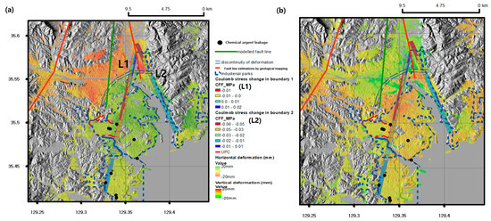
Figure 10.
Horizontal (a) and vertical deformations (b) together with the hazard context (e.g., chemical leakage cases) during the 2017–2018 period. The extent of UPC and other industrial parks together with the outcomes from the CFF analysis using Ulsan fault parameters are also demonstrated.
Even considering the design margins of pipelines and facilities, such stress fields could result in dangerous situations upon the occurrence of even relatively insignificant earthquakes. In addition, half the total industrial park area has suffered 1-cm level surface deformation in both the horizontal and vertical directions, perhaps due to migration of the Ulsan fault. According to the classification of fault activation by Matsuda [72], such a deformation rate corresponds to the A class (10–1 m/Ka), which can cause major earthquake damage; thus, it is an area of high risk for future potential seismic activities. It is not easy task to estimate the magnitude and consequent damage of future earthquakes as there remains ongoing debate about the relationship among slip rates, dimensions of fault lines, and magnitudes of potential earthquakes [73]. Because the locations of potential seismic sources are not localized with the available information, quantitative hazard assessment employing probabilistic approaches is further proposed. Seismic hazard assessments are normally conducted by either deterministic seismic hazard assessment or PSHA [74]. As deterministic seismic hazard assessment considers a small number of source scenarios and the largest ground motion, it does not fit with the case of this study. On the contrary, PSHA includes all possible scenarios and computes the synthesized probability of certain thresholds of ground motion. Considering the uncertainty of the earthquakes that may be induced by the Ulsan fault line, we employed PSHA and its S/W implementation, called the R-CRISIS (http://www.r-crisis.com/) [75,76] to extract a potential hazard map. Combined with the seismic source extracted from the GBIS model (Table 5) and the historical earthquake record around the Ulsan fault line (Figure 11a), which was integrated into the Gutenberg–Richter model [77], we calculated the risk map around the Ulsan City area, as demonstrated in Figure 11b–d. Note that the modified Gutenberg–Richter method [78] implemented in R-CRISIS establishes a seismicity model associated with occurrence probability of earthquake of considerable magnitudes within a certain frame time period. In this study, the time frame was established as 50 years, considering the recurrence time period of the major earthquakes in the target area. This may have some implications on the potential activation period of the Yangsan-Ulsan faults, but is not strongly supported by the ground works owing to absence of long-term study of the Yangsan-Ulsan faults. Thus, our risk assessment needs to be considered as a case study based on the scenario to assess the potential risk, rather than a robust estimation. The risk maps represented by the intensity values in a 10% exceedance probability demonstrated that (1) all industrial parks, in particular UPC, belong to the highest risk area; (2) the peak time of seismic risk is around ten years, as shown in Figure 11c. Regarding the confidences of modelled parameters employed for the risk assessment, it is worth noting that the recent active fault studies [31,79] around Ulsan reconstructed the migrating structure similar to this study. Thus, the PSHA outcomes in this study can be used for future safety planning as well as the establishment of new industrial regulations.
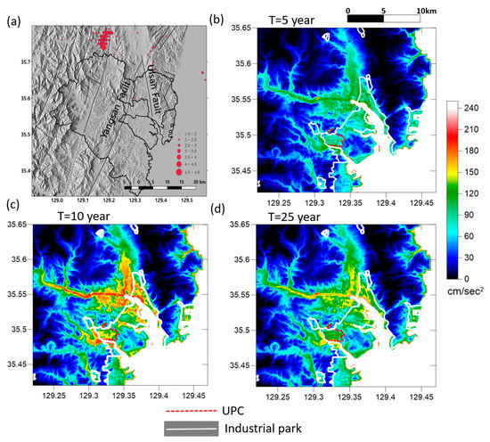
Figure 11.
(a) Input seismic activity map for earthquake risk estimation for the 2000–2018 period; (b–d) risk map with the intensity values using R-CRISIS PSHA S/W over the Ulsan city area for the next 5 years (b), 10 years (c), and 25 years (d). Threshold magnitude 3.5 was applied with 10% exceedance probability.
Overall, both methods employed in this study estimated that the industrial parks of Ulsan, especially UPC, are susceptible to future potential earthquakes induced by the activated Ulsan fault. Such high precision 3D PS algorithms together with high resolution X band SAR imagery [80], are required to trace the stability of individual industrial components. Our results also showed a vertical deformation anomaly in the city area (Unit 7, P10, and P13 in Figure 6), which may have been induced by the recent construction of skyscraper clusters. Some isolated deformation spots observed within Ulsan city areas may be indicative of potential future risks (e.g., sink holes). The major concern revealed in this study is the strong migration trend of the Ulsan fault, which may imply a triggered slip of a large earthquake as discussed in previous studies [81,82].
6. Conclusions and Future Work
This study was motivated by two recent earthquakes that occurred in the southeastern part of the Korean Peninsula. Owing to their unprecedented magnitudes and proximity to Ulsan, the major heavy chemical industrial hub of Korea, we conducted InSAR time series analysis over Ulsan city area and the surrounding Ulsan and Yangsan faults. The two major conclusions of this geodetic campaign are: 1) the Ulsan fault was found to be far more active than the stable Yangsan fault; and 2) heavy surface deformation in the Ulsan area is not a consequence of the two major earthquakes, but is caused by independent tectonic interactions, mainly along the Ulsan fault. Because this deformation may pose a greater threat to the fragile industrial facilities of Ulsan than did the coupled effects of both earthquakes, we conducted deformation source analyses via geophysical inversion and further employed Coulomb stress simulations and probabilistic analysis for the quantitative hazard mapping. It appears that a large portion of the chemical pipeline with toxic agents and subtle production facilities are located within the influence of undergoing/future surface deformations. Based on the outcomes of this study, we very strongly propose that the most significant concern from plausible seismic activity in this area is the stability of the Ulsan fault and the consequent risks posed on industrial parks and surrounding residential areas. To better prepare against such a potential hazard, continuous monitoring using high precision geodetic techniques is essential.
We present this study as a model case to monitor the threat to industrial safety from potential surface deformation disasters. The remote sensing/geophysical techniques and hazard assessment procedures in this study proved the validity of a continuous monitoring scheme for ongoing subtle deformation that may induce various risks or imply significant future earthquake damage. Similar or improved approaches can play a role in preparations as well as in post-event investigations of seismic disasters at dense industrial hubs.
Author Contributions
H.-W.Y. conducted DInSAR analysis and wrote the major part of paper. J.-R.K. designed the research structure and conducted geophysical modelling together with writing. H.Y. and Y.C. charged of collections and processing of GPS and involved writing. J.Y. contributed in SAR processing part.
Funding
The contributions by Hey-Won Yun and JungHum Yu in this study were supported by the internal research support scheme of National Disaster Management Research Institute.
Acknowledgments
The authors thank for the useful comments by anonymous reviewers and the editors which were greatly helpful for the improvement of this study. The authors acknowledge the computer resource by the engineering equipment grant of University of Seoul.
Conflicts of Interest
The authors declare no conflict of interest.
References
- Arciniegas, G.A.; Bijker, W.; Kerle, N.; Tolpekin, V.A. Coherence-and amplitude-based analysis of seismogenic damage in Bam, Iran, using ENVISAT ASAR data. IEEE Trans. Geosci. Remote Sens. 2007, 45, 1571–1581. [Google Scholar] [CrossRef]
- Stramondo, S.; Bignami, C.; Chini, M.; Pierdicca, N.; Tertulliani, A. Satellite radar and optical remote sensing for earthquake damage detection: Results from different case studies. Int. J. Remote Sens. 2006, 27, 4433–4447. [Google Scholar] [CrossRef]
- Brunner, D.; Lemoine, G.; Bruzzone, L. Earthquake damage assessment of buildings using VHR optical and SAR imagery. IEEE Trans. Geosci. Remote Sens. 2010, 48, 2403–2420. [Google Scholar] [CrossRef]
- Nissen, E.; Elliott, J.R.; Sloan, R.A.; Craig, T.J.; Funning, G.J.; Hutko, A.; Wright, T.J. Limitations of rupture forecasting exposed by instantaneously triggered earthquake doublet. Nat. Geosci. 2016, 9, 330. [Google Scholar] [CrossRef]
- Kim, Y.; Rhie, J.; Kang, T.S.; Kim, K.H.; Kim, M.; Lee, S.J. The 12 September 2016 Gyeongju earthquakes: 1. Observation and remaining questions. Geosci. J. 2016, 20, 747–752. [Google Scholar] [CrossRef]
- Kim, K.H.; Kang, T.S.; Rhie, J.; Kim, Y.; Park, Y.; Kang, S.Y.; Kong, C. The 12 September 2016 Gyeongju earthquakes: 2. Temporary seismic network for monitoring aftershocks. Geosci. J. 2016, 20, 753–757. [Google Scholar] [CrossRef]
- Kim, Y.S.; Kim, T.; Kyung, J.B.; Cho, C.S.; Choi, J.H.; Choi, C.U. Preliminary study on rupture mechanism of the 9.12 Gyeongju earthquake. J. Geol. Soc. Korea 2017, 53, 407–422. [Google Scholar] [CrossRef]
- Grigoli, F.; Cesca, S.; Rinaldi, A.P.; Manconi, A.; López-Comino, J.A.; Clinton, J.F.; Wiemer, S. The November 2017 Mw 5.5 Pohang earthquake: A possible case of induced seismicity in South Korea. Science 2018, 360, 1003–1006. [Google Scholar] [CrossRef]
- Kim, K.H.; Ree, J.H.; Kim, Y.; Kim, S.; Kang, S.Y.; Seo, W. Assessing whether the 2017 Mw 5.4 Pohang earthquake in South Korea was an induced event. Science 2018, 360, 1007–1009. [Google Scholar] [CrossRef]
- Chen, Y.; Zhang, M.; Guo, P.; Jiang, J. Investigation and analysis of historical Domino effects statistic. Procedia Eng. 2012, 45, 152–158. [Google Scholar] [CrossRef]
- Krausmann, E.; Cruz, A.M.; Affeltranger, B. The impact of the 12 May 2008 Wenchuan earthquake on industrial facilities. J. Loss Prev. Process Ind. 2010, 23, 242–248. [Google Scholar] [CrossRef]
- Nishi, H. Damage on hazardous materials facilities. In Proceedings of the International Symposium on Engineering Lessons Learned from the 2011 Great East Japan Earthquake, Tokyo, Japan, 1–4 March 2012. [Google Scholar]
- Sezen, H.; Whittaker, A.S. Seismic performance of industrial facilities affected by the 1999 Turkey earthquake. J. Perform. Constr. Facil. 2006, 20, 28–36. [Google Scholar] [CrossRef]
- Suzuki, K. Earthquake damage to industrial facilities and development of seismic and vibration control technology. J. Syst. Des. Dyn. 2008, 2, 2–11. [Google Scholar] [CrossRef][Green Version]
- Lindell, M.K.; Perry, R.W. Hazardous materials releases in the Northridge earthquake: Implications for seismic risk assessment. Risk Anal. 1997, 17, 147–156. [Google Scholar] [CrossRef]
- Lanzano, G.; Santucci de Magistris, F.; Fabbrocino, G.; Salzano, E. An observational analysis of seismic vulnerability of industrial pipelines. Chem. Eng. Trans. 2012, 26, 567–572. [Google Scholar]
- Campedel, M. Analysis of major industrial accidents triggered by natural events reported in the principal available chemical accident databases. Rep. EUR 2008, 23391. Available online: http://publications.jrc.ec.europa.eu/repository/handle/JRC42281 (accessed on 19 May 2019).
- Sengul, H.; Santella, N.; Steinberg, L.J.; Cruz, A.M. Analysis of hazardous material releases due to natural hazards in the United States. Disasters 2012, 36, 723–743. [Google Scholar] [CrossRef]
- Seed, H.B.; Idriss, I.M. Analysis of soil liquefaction: Niigata earthquake. J. Soil Mech. Found. Div. 1967, 93, 83–108. [Google Scholar]
- Nath, S.K.; Srivastava, N.; Ghatak, C.; Adhikari, M.D.; Ghosh, A.; Ray, S.S. Earthquake induced liquefaction hazard, probability and risk assessment in the city of Kolkata, India: Its historical perspective and deterministic scenario. J. Seismolog. 2018, 22, 35–68. [Google Scholar] [CrossRef]
- Tamari, Y.; Hyodo, J.; Ichii, K.; Nakama, T.; Hosoo, A. Developments in Earthquake Geotechnics; Springer: Berlin, Germany, 2018; Volume 11, pp. 201–217. ISBN 978-3-319-62068-8. [Google Scholar]
- Simons, M.; Fialko, Y.; Rivera, L. Coseismic deformation from the 1999 M w 7.1 Hector Mine, California, earthquake as inferred from InSAR and GPS observations. Bull. Seismol. Soc. Am. 2002, 92, 1390–1402. [Google Scholar] [CrossRef]
- Delouis, B.; Nocquet, J.M.; Vallée, M. Slip distribution of the February 27, 2010 Mw = 8.8 Maule earthquake, central Chile, from static and high-rate GPS, InSAR, and broadband teleseismic data. Geophys. Res. Lett. 2010, 37. [Google Scholar] [CrossRef]
- Klein, E.; Vigny, C.; Fleitout, L.; Grandin, R.; Jolivet, R.; Rivera, E.; Métois, M. A comprehensive analysis of the Illapel 2015 Mw8. 3 earthquake from GPS and InSAR data. Earth Planet. Sci. Lett. 2017, 469, 123–134. [Google Scholar] [CrossRef]
- Natsuaki, R.; Nagai, H.; Tomii, N.; Tadono, T. Sensitivity and Limitation in Damage Detection for Individual Buildings Using InSAR Coherence—A Case Study in 2016 Kumamoto Earthquakes. Remote Sens. 2018, 10, 245. [Google Scholar] [CrossRef]
- Yun, S.H.; Hudnut, K.; Owen, S.; Webb, F.; Simons, M.; Sacco, P.; Milillo, P. Rapid Damage Mapping for the 2015 M w 7.8 Gorkha Earthquake Using Synthetic Aperture Radar Data from COSMO–SkyMed and ALOS-2 Satellites. Seismol. Res. Lett. 2015, 86, 1549–1556. [Google Scholar] [CrossRef]
- Chini, M.; Albano, M.; Saroli, M.; Pulvirenti, L.; Moro, M.; Bignami, C.; Stramondo, S. Coseismic liquefaction phenomenon analysis by COSMO-SkyMed: 2012 Emilia (Italy) earthquake. Int. J. Appl. Earth Obs. Geoinf. 2015, 39, 65–78. [Google Scholar] [CrossRef]
- Baker, J.W. An introduction to probabilistic seismic hazard analysis. White Paper Version 2 2013, 79. [Google Scholar]
- Okada, A.; Watanabe, M.; Sato, H.; Jun, M.S.; Jo, W.R.; Kim, S.K.; Oike, K. Active fault topography and trench survey in the central part of the Yangsan fault, Southeast Korea. Geogr. J. 1994, 103, 111–126. [Google Scholar] [CrossRef]
- Kyung, J.B.; Lee, K.H. Active fault study of the Yangsan fault system and Ulsan fault system, southeastern part of the Korean Peninsula. J. Korean Geophys. Soc. 2006, 9, 219–230. [Google Scholar]
- Kyung, J.B. Paleoseismological study and evaluation of maximum earthquake magnitude along the Yangsan and Ulsan Fault Zones in the Southeastern Part of Korea. Geophys. Geophys. Explor. 2010, 13, 187–197. [Google Scholar]
- Choi, S.J.; Jeon, J.S.; Choi, J.H.; Kim, B.; Ryoo, C.R.; Hong, D.G.; Chwae, U. Estimation of possible maximum earthquake magnitudes of Quaternary faults in the southern Korean Peninsula. Quat. Int. 2014, 344, 53–63. [Google Scholar] [CrossRef]
- Wright, T.J.; Lu, Z.; Wicks, C. Source model for the Mw 6.7, 23 October 2002, Nenana Mountain Earthquake (Alaska) from InSAR. Geophys. Res. Lett. 2003, 30. [Google Scholar] [CrossRef]
- Fialko, Y.; Simons, M.; Agnew, D. The complete (3-D) surface displacement field in the epicentral area of the 1999 Mw7. 1 Hector Mine earthquake, California, from space geodetic observations. Geophys. Res. Lett. 2001, 28, 3063–3066. [Google Scholar] [CrossRef]
- Galloway, D.L.; Hudnut, K.W.; Ingebritsen, S.E.; Phillips, S.P.; Peltzer, G.; Rogez, F.; Rosen, P.A. Detection of aquifer system compaction and land subsidence using interferometric synthetic aperture radar, Antelope Valley, Mojave Desert, California. Water Resour. Res. 1998, 34, 2573–2585. [Google Scholar] [CrossRef]
- Osmanoğlu, B.; Dixon, T.H.; Wdowinski, S.; Cabral-Cano, E.; Jiang, Y. Mexico City subsidence observed with persistent scatterer InSAR. Int. J. Appl. Earth Obs. Geoinf. 2011, 13, 1–12. [Google Scholar] [CrossRef]
- Ye, X.; Kaufmann, H.; Guo, X.F. Landslide monitoring in the Three Gorges area using D-InSAR and corner reflectors. Photogramm. Eng. Remote Sens. 2004, 70, 1167–1172. [Google Scholar] [CrossRef]
- Yin, Y.; Zheng, W.; Liu, Y.; Zhang, J.; Li, X. Integration of GPS with InSAR to monitoring of the Jiaju landslide in Sichuan, China. Landslides 2010, 7, 359–365. [Google Scholar] [CrossRef]
- Zhao, C.; Lu, Z.; Zhang, Q.; de La Fuente, J. Large-area landslide detection and monitoring with ALOS/PALSAR imagery data over Northern California and Southern Oregon, USA. Remote Sens. Environ. 2012, 124, 348–359. [Google Scholar] [CrossRef]
- Gabriel, A.K.; Goldstein, R.M.; Zebker, H.A. Mapping small elevation changes over large areas: Differential radar interferometry. J. Geophys. Res. Solid Earth 1989, 94, 9183–9191. [Google Scholar] [CrossRef]
- Ding, X.L.; Li, Z.W.; Zhu, J.J.; Feng, G.C.; Long, J.P. Atmospheric effects on InSAR measurements and their mitigation. Sensors 2008, 8, 5426–5448. [Google Scholar] [CrossRef]
- Torres, R.; Snoeij, P.; Geudtner, D.; Bibby, D.; Davidson, M.; Attema, E.; Traver, I.N. GMES Sentinel-1 mission. Remote Sens. Environ. 2012, 120, 9–24. [Google Scholar] [CrossRef]
- Kim, J.R.; Yun, H.W.; Van Gasselt, S.; Choi, Y.S. Error-Regulated Multi-Pass DInSAR Analysis for Landslide Risk Assessment. Photogramm. Eng. Remote Sens. 2018, 84, 189–202. [Google Scholar] [CrossRef]
- Ferretti, A.; Prati, C.; Rocca, F. Nonlinear Subsidence Rate Estimation Using Permanent Scatterers in Differential SAR Interferometry. IEEE Trans. Geosci. Remote Sens. 2000, 38, 2202–2212. [Google Scholar] [CrossRef]
- Ferretti, A.; Fumagalli, A.; Novali, F.; Prati, C.; Rocca, F.; Rucci, A. A new algorithm for processing interferometric data-stacks: SqueeSAR. IEEE Trans. Geosci. Remote Sens. 2011, 49, 3460–3470. [Google Scholar] [CrossRef]
- Berardino, P.; Fornaro, G.; Lanari, R.; Sansosti, E. A New Algorithm for Surface Deformation Monitoring Based on Small Baseline Differential Interferograms. IEEE Trans. Geosci. Remote Sens. 2002, 40, 2375–2383. [Google Scholar] [CrossRef]
- Gong, W.; Thiele, A.; Hinz, S.; Meyer, F.J.; Hooper, A.; Agram, P.S. Comparison of small baseline Interferometric SAR processors for estimating ground deformation. Remote Sens. 2016, 8, 330. [Google Scholar] [CrossRef]
- Tadono, T.; Ishida, H.; Oda, F.; Naito, S.; Minakawa, K.; Iwamoto, H. Precise global DEM generation by ALOS PRISM. ISPRS Ann. Photogramm. Remote Sens. Spat. Inf. Sci. 2014, 2, 71. [Google Scholar]
- Dach, R.; Lutz, S.; Walser, P.; Fridez, P. Bernese GNSS Software Version 5.2; Astronomical Institute, University of Bern: Bern, Switzerland, 2015. [Google Scholar]
- Ostini, L.; Dach, R.; Meindl, M.; Schaer, S.; Hugentobler, U. FODITS: A new tool of the Bernese GPS software to analyze time series. In Proceedings of the EUREF 2008 Symposium, Brussels, Belgium, 18–21 June 2008. [Google Scholar]
- Sohn, D.H.; Kim, D.S.; Park, K.D. A Study on GNSS Data Pre-processing for Analyzing Geodetic Effects on Crustal Deformation due to the Earthquake. J. Korean Soc. Geospat. Inf. Syst. 2015, 23, 47–54. [Google Scholar]
- Kim, D.; Park, K.D.; Ha, J.; Sohn, D.H.; Won, J. Geodetic analysis of postseismic crustal deformations occurring in South Korea due to the Tohoku-Oki earthquake. KSCE J. Civ. Eng. 2016, 20, 2885–2892. [Google Scholar] [CrossRef]
- Hooper, A.; Bekaert, D.; Spaans, K.; Arıkan, M. Recent advances in SAR interferometry time series analysis for measuring crustal deformation. Tectonophysics 2012, 514, 1–13. [Google Scholar] [CrossRef]
- Ferretti, A.; Prati, C.; Rocca, F. Permanent scatterers in SAR interferometry. IEEE Trans. Geosci. Remote Sens. 2001, 39, 8–20. [Google Scholar] [CrossRef]
- Bekaert, D.P.S.; Walters, R.J.; Wright, T.J.; Hooper, A.J.; Parker, D.J. Statistical comparison of InSAR tropospheric correction techniques. Remote Sens. Environ. 2015, 170, 40–47. [Google Scholar] [CrossRef]
- Jung, J.; Kim, D.J.; Park, S.E. Correction of atmospheric phase screen in time series InSAR using WRF model for monitoring volcanic activities. IEEE Trans. Geosci. Remote Sens. 2014, 52, 2678–2689. [Google Scholar] [CrossRef]
- Li, Z.; Fielding, E.J.; Cross, P. Integration of InSAR time-series analysis and water-vapor correction for mapping postseismic motion after the 2003 Bam (Iran) earthquake. IEEE Trans. Geosci. Remote Sens. 2009, 47, 3220–3230. [Google Scholar]
- Crosetto, M.; Monserrat, O.; Cuevas-González, M.; Devanthéry, N.; Crippa, B. Persistent scatterer interferometry: A review. ISPRS J. Photogramm. Remote Sens. 2016, 115, 78–89. [Google Scholar] [CrossRef]
- Crosetto, M.; Monserrat, O.; Iglesias, R.; Crippa, B. Persistent scatterer interferometry. Photogramm. Eng. Remote Sens. 2010, 76, 1061–1069. [Google Scholar] [CrossRef]
- Hooper, A.; Segall, P.; Zebker, H. Persistent scatterer InSAR for crustal deformation analysis, with application to Volcán Alcedo, Galápagos. J. Geophys. Res. 2007, 112, 19. [Google Scholar] [CrossRef]
- Shanker, P.; Casu, F.; Zebker, H.A.; Lanari, R. Comparison of persistent scatterers and small baseline time-series InSAR results: A case study of the San Francisco Bay Area. IEEE Trans. Geosci. Remote Sens. 2011, 8, 592–596. [Google Scholar] [CrossRef]
- Wright, T.; Parsons, B.; Fielding, E. Measurement of interseismic strain accumulation across the North Anatolian Fault by satellite radar interferometry. Geophys. Res. Lett. 2001, 28, 2117–2120. [Google Scholar] [CrossRef]
- Motagh, M.; Hoffmann, J.; Kampes, B.; Baes, M.; Zschau, J. Strain accumulation across the Gazikoy–Saros segment of the North Anatolian Fault inferred from Persistent Scatterer Interferometry and GPS measurements. Earth Planet. Sci. Lett. 2007, 255, 432–444. [Google Scholar] [CrossRef]
- Walters, R.J.; Holley, R.J.; Parsons, B.; Wright, T.J. Interseismic strain accumulation across the North Anatolian Fault from Envisat InSAR measurements. Geophys. Res. Lett. 2011, 38. [Google Scholar] [CrossRef]
- Bagnardi, M.; Hooper, A. Inversion of surface deformation data for rapid estimates of source parameters and uncertainties: A Bayesian approach. Geochem. Geophys. Geosyst. 2018, 19, 2194–2211. [Google Scholar] [CrossRef]
- Hastings, W.K. Monte Carlo sampling methods using Markov chains and their applications. Biometrika 1970, 57, 97–109. [Google Scholar] [CrossRef]
- Mosegaard, K.; Tarantola, A. Monte Carlo sampling of solutions to inverse problems. Persistent scatterer InSAR for crustal deformation analysis. J. Geophys. Res. Solid Earth 1995, 100, 12431–12447. [Google Scholar] [CrossRef]
- Albano, M.; Polcari, M.; Bignami, C.; Moro, M.; Saroli, M.; Stramondo, S. Did Anthropogenic Activities Trigger the 3 April 2017 Mw 6.5 Botswana Earthquake? Remote Sens. 2017, 9, 1028. [Google Scholar] [CrossRef]
- Han, S.R.; Park, J.; Kim, Y.S. Evolution modeling of the Yangsan-Ulsan fault system with stress changes. J. Geol. Soc. Korea 2009, 45, 361–377. [Google Scholar]
- King, G.C.; Stein, R.S.; Lin, J. Static stress changes and the triggering of earthquakes. Bull. Seismol. Soc. Am. 1994, 84, 935–953. [Google Scholar]
- Stein, R.S. The role of stress transfer in earthquake occurrence. Nature 1999, 402, 605. [Google Scholar] [CrossRef]
- Matsuda. Earthquake magnitude and return period from active fault. J. Seismol. Soc. Jpn. 1975, 28, 269–283. [Google Scholar]
- Leonard, M. Earthquake fault scaling: Self-consistent relating of rupture length, width, average displacement, and moment release. Bull. Seismol. Soc. Am. 2010, 100, 1971–1988. [Google Scholar] [CrossRef]
- McGuire, R.K. Deterministic vs. probabilistic earthquake hazards and risks. Soil Dyn. Earthq. Eng. 2001, 21, 377–384. [Google Scholar] [CrossRef]
- Ordaz, M.; Martinelli, F.; Meletti, C.; D’Amico, V. CRISIS2012: An Updated Tool to Compute Seismic Hazard. In AGU Spring Meeting Abstracts; American Geophysical Union: Washington, DC, USA, 2013. [Google Scholar]
- Duzgun, H.S.B.; Yucemen, M.S.; Kalaycioglu, H.S.; Celik, K.; Kemec, S.; Ertugay, K.; Deniz, A. An integrated earthquake vulnerability assessment framework for urban areas. Nat. Hazards 2011, 59, 917. [Google Scholar] [CrossRef]
- Christensen, K.; Olami, Z. Variation of the Gutenberg-Richter b values and nontrivial temporal correlations in spring-block model for earthquakes Persistent scatterer InSAR for crustal deformation analysis, with application to Volcán Alcedo, Galápagos. J. Geophys. Res. Solid Earth 1992, 97, 8729–8735. [Google Scholar] [CrossRef]
- Cornell, C.A.; Vanmarke, E.H. The major influences on seismic risk. In Proceedings of the 3rd World Conference on Earthquake Engineering, Santiago, Chile, 13–18 January 1969. [Google Scholar]
- Choi, J.H.; Yang, S.J.; Han, S.R.; Kim, Y.S. Fault zone evolution during Cenozoic tectonic inversion in SE Korea. J. Asian Earth Sci. 2015, 98, 167–177. [Google Scholar] [CrossRef]
- Perissin, D. Validation of the submetric accuracy of vertical positioning of PSs in C-band. IEEE Trans. Geosci. Remote Sens. 2008, 5, 502–506. [Google Scholar] [CrossRef]
- Le Béon, M.; Huang, M.H.; Suppe, J.; Huang, S.T.; Pathier, E.; Huang, W.J.; Hu, J.C. Shallow geological structures triggered during the Mw 6.4 Meinong earthquake, southwestern Taiwan. Terr. Atmos. Ocean. Sci. 2010, 28, 663–681. [Google Scholar] [CrossRef]
- Rymer, M.J.; Treiman, J.A.; Kendrick, K.J.; Lienkaemper, J.J.; Weldon, R.J.; Bilham, R.; Irvine, P.J. Triggered Surface Slips in Southern California Associated with the 2010 El Mayor-Cucapah, Baja California, Mexico, Earthquake; US Geological Survey: Reston, VA, USA, 2011.
© 2019 by the authors. Licensee MDPI, Basel, Switzerland. This article is an open access article distributed under the terms and conditions of the Creative Commons Attribution (CC BY) license (http://creativecommons.org/licenses/by/4.0/).