Noise Removal Based on Tensor Modelling for Hyperspectral Image Classification

Abstract

With the current state-of-the-art computer aided manufacturing tools, the spatial resolution of hyperspectral sensors is becoming increasingly higher thus making it easy to obtain much more detailed information of the scene captured. However, the improvement of the spatial resolution also brings new challenging problems to address with signal dependent photon noise being one of them. Unlike the signal independent thermal noise, the variance of photon noise is dependent on the signal, therefore many denoising methods developed for the stationary noise cannot be applied directly to the photon noise. To make things worse, both photon and thermal noise coexist in the captured hyperspectral image (HSI), thus making it more difficult to whiten noise. In this paper, we propose a new denoising framework to cope with signal dependent nonwhite noise (SDNW), Pre-estimate—Whitening—Post-estimate (PWP) loop, to reduce both photon and thermal noise in HSI. Previously, we proposed a method based on multidimensional wavelet packet transform and multi-way Wiener filter which performs both white noise and spectral dimensionality reduction, referred to as MWPT-MWF, which was restricted to white noise. We get inspired from this MWPT-MWF to develop a new iterative method for reducing photon and thermal noise. Firstly, the hyperspectral noise parameters estimation (HYNPE) algorithm is used to estimate the noise parameters, the SD noise is converted to an additive white Gaussian noise by pre-whitening procedure and then the whitened HSI is denoised by the proposed method SDNW-MWPT-MWF. As comparative experiments, the Multiple Linear Regression (MLR) based denoising method and tensor-based Multiway Wiener Filter (MWF) are also used in the denoising framework. An HSI captured by Reflective Optics System Imaging Spectrometer (ROSIS) is used in the experiments and the denoising performances are assessed from various aspects: the noise whitening performance, the Signal-to-Noise Ratio (SNR), and the classification performance. The results on the real-world airborne hyperspectral image HYDICE (Hyperspectral Digital Imagery Collection Experiment) are also presented and analyzed. These experiments show that it is worth taking into account noise signal-dependency hypothesis for processing HYDICE and ROSIS HSIs.

1. Introduction

Hyperspectral images consist of a considerably large number of narrow spectral bands which are uniformly distributed over a wide spectral range. For each pixel, the almost continuous spectral signature adds the third orthogonal spectral dimension to the two-dimensional spatial domain and constitutes the well-known 3D data cube. Thus, hyperspectral signatures offer the capability to identify and discriminate ground cover types. To benefit from the additional spectral dimension, specific processing methods of hyperspectral images, for instance spectral signatures unmixing, target detection and classification, etc., have been developed. For these methods to operate well, the reduction of the noise affecting hyperspectral images (HSIs) should be incorporated into them.

The noise in HSIs can be distinguished into two classes [1]: random noise and fixed pattern noise. Photon and thermal noise are examples of random noise in HSIs, while striping, periodic and interference noise are examples of fixed pattern noise, which is generated by errors in the calibration process and can be removed from the HSI by suitable procedures [2]. However, random noise, due to its stochastic nature, cannot be removed by those procedures and influences the performance of the algorithms adopted in hyperspectral data exploitation. Note that, in this paper, we only focus on the random noise and will later refer to it as noise. For sensors used in hyperspectral imagery, the theory predicts that random noise mainly comes from two aspects: signal-independent (SI) electronic noise and signal-dependent (SD) photon noise [3]. The widely accepted SI noise model is white Gaussian one [1,3]. In [4,5], it was shown that the SI noise in some HSIs is colored, i.e., spectrally non-white. With the improvement of the sensitivity in the electronic components [6], the resolution of the charged coupled device (CCD) camera has improved significantly, so that the photon noise has become as dominant as the signal-independent electronic noise in HSI data collected by new-generation hyperspectral sensors [7,8,9,10]. In this case, the assumption of additive and stationary noise model is not appropriate although this hypothesis is plausible for HSIs where the SI noise is dominant while SD noise, which depends on the useful signal level, is negligible. Therefore, in this paper, we use the widely accepted noise model in [7,8,9,10] including both signal-dependent and signal-independent noise. There are few denoising algorithms based on the photon noise model. The tensor-based denoising methods were proposed only for the white noise situation. According to the different statistical properties of SI and SD noise, in this paper, we propose a method to remove the SD photon noise as well as the SI thermal noise in the HSI.

In the literature, two widely used models for the random noise in HSIs are the additive white noise along both spectral and spatial dimensions [8,11,12,13,14], and the Additive White Gaussian Noise (AWGN) along the spatial dimensions but non-stationary in the spectral dimension [15,16]; these are pretty reasonable processes when the thermal noise is dominant [8]. However, when the SD photon noise is taken into account, these two noise models become appropriate. The SD photon noise in digital images was discussed in [17,18], where the noise parameters were estimated by utilizing a scatter plot-based estimation procedure. Nonetheless, the discussion of these two papers was only limited to the pure SD noise, which is not suitable for the noise in HSIs. A more accurate generalized SD noise model for digital images was introduced in [19], where the noise parameters were estimated by the Linear Minimum Mean Square Error (LMMSE) in the wavelet domain. In addition, the same noise model was employed in [20] under the name Poissonian-Gaussian noise model, where the noise in HSIs was modeled as two parts: the Poissonian part for modeling the photon noise and the Gaussian part for modeling the remaining stationary distribution in the output data. Images were firstly transformed into the wavelet domain; then, the expectation/standard-deviation pairs were estimated by employing a local estimation method. Finally, the Maximum Likelihood (ML) method was applied to the locally estimated expectation/standard-deviation pairs to estimate the global parameters. Based on the generalized SD noise model, a scatter plot-based estimation method was proposed in [7] to estimate the parameters of the noise generated by the new-generation imaging spectrometers.

The generalized SD noise model was then introduced in the HSI framework in [3]. In this paper, the 2D fractal Brownian motion (fBm) model was employed as a statistical model for intra-band image texture correlation, which has made it possible to estimate additive noise variance locally both from homogeneous and textural images Scanning Widow (SW). Then, the noise parameters were estimated by a linear fit in each band. The spectral textural correlation was also considered, and each SW in a Multicomponent Scanning Window (MSW) was treated as a mixture of fBm-samples and noise. Finally, the global noise parameters were estimated by ML estimation.

The generalized SD noise model was also used in [8], where the HYperspectral Noise Parameter Estimation (HYNPE) algorithm was proposed. Unlike [3], HYNPE utilized the assumption that the noise in each band after being whitened followed a standard Gaussian distribution. The joint probability density function (PDF) of the whitened noise values was used to form the ML criterion. Nonetheless, the signal and noise values were assumed to be known in the ML criterion, which was not true in practical situations. Hence, the MLR-theory based approach was exploited to estimate them. However, MLR calculates the parameters by minimizing the Least Square Error (LSE), which is a biased estimator when the noise is not white. Thus, the estimates of MLR are not accurate in HYNPE, leading to the inaccuracy of the final parameter estimates. In this paper, we investigate the relevance of a new denoising framework for reducing simultaneously the SD photon noise and the SI thermal noise in HSIs on classification [21]. Considering that the noise variance is entangled with the signal, a denoising loop is proposed to remove the noise from HSIs. Each iteration of the loop consists three steps: firstly, we do the pre-estimate, i.e., use MWPT-MWF to directly denoise the HSI containing the photon and thermal noise. Secondly, use the pre-estimate to estimate the noise parameters by employing the ML criterion, and then whiten the noise. Finally, apply MWPT-MWF to the whitened HSIs to obtain the post-estimate. Then, in the next iteration, use the post-estimate of the last iteration as the pre-estimate of current iteration. After several iterations, the HSIs will be well denoised and the resulting classification results are improved.

The remainder of this paper is organized as follows: Section 2 gives the signal model used in this paper. Appendix A presents the Multilinear Algebra Tools. Appendix B overviews the HYNPE algorithm. Appendix C presents the MWPT-MWF method. Section 3 presents the proposed iterative denoising method: considering that the noise variance is dependent on the signal, a denoising loop is proposed to remove the noise from HSIs. Each iteration of the loop consists of three steps: (i) we perform a pre-estimation, i.e., use MWPT-MWF [22,23] to directly denoise the HSI containing the photon and thermal noise, (ii) we use the pre-estimation process to estimate the noise parameters by employing the ML criterion, and then whiten the noise and (iii) we apply MWPT-MWF to the whitened HSIs to obtain the post-estimate results. Then in the next iteration, we use the post-estimate of the last iteration as the pre-estimate of current iteration. After several iterations, the HSIs will be well denoised. Section 4 gives some comparative experimental results. The real-world HSI reflective optics system imaging spectrometer (ROSIS) is used in the experiments to evaluate the performances of denoising and classification processes. Finally, Section 6 provides details of the conclusions of the research undertaken.

In this paper, we denote by

$x\in \mathbb{R}$	a scalar
$\mathbf{x}\in {\mathbb{R}}^{I_1}$	a vector
$\mathbf{X}\in {\mathbb{R}}^{I_1\times I_2}$	a matrix
$\mathcal{X}\in {\mathbb{R}}^{I_1\times I_2\times \dots I_N}$	a N-order tensor
${\mathbf{X}}_n$	n-mode unfolding matrix
${\mathcal{X}}_{\mathcal{X}\mathcal{T}}$	a tensor obtained by calculating the square root of each element of $\mathcal{X}$
$I_n$	n-mode dimension
$\parallel \mathbf{X}\parallel$	the Frobenius norm of $\mathbf{X}$
∘	the vector outer product
⊙	the Khatri-Rao product
⊛	the Hadamard product
$<\mathcal{X},\mathcal{Y}>$	the inner product between $\mathcal{X}$ and $\mathcal{Y}$
$\mathrm{E}[·]$	the mathematical expectation
${(.)}^T$	the transposition.

2. Signal Modeling with Thermal and Photon Noise

An HSI is a three-dimensional data cube and can be modeled as a tensor $\mathcal{R}\in {\mathbb{R}}^{I_1\times I_2\times I_3}$, with the first two dimensions being the spatial domain and with the third dimension being the spectral domain. In fact, a hyperspectral sensor captures a HSI as a series of two-dimensional images of the spatial domain by a sensor array. By extending the data model in [7] to the 3D representation, a noisy HSI can be expressed as a third order tensor $\mathcal{R}\in {\mathbb{R}}^{I_1\times I_2\times I_3}$ composed of a multidimensional signal $\mathcal{X}\in {\mathbb{R}}^{I_1\times I_2\times I_3}$ impaired by an additive random noise $\mathcal{N}\in {\mathbb{R}}^{I_1\times I_2\times I_3}$:

$$\mathcal{R}=\mathcal{X}+\mathcal{N},$$

(1)

where $\mathcal{N}$ accounts for both thermal and photon noise and its variance depends on the pixel $x_{i_1,i_2,i_3}$ in the useful signal $\mathcal{X}$. The photon noise is caused by the random fluctuation of photon flux arriving at the CCD sensor, and it follows a Poisson model [24]. As the pixel size becomes smaller in the new-generation hyperspectral sensor, the number of photons that reach a pixel per unit time becomes smaller as well. Hence, the photon noise cannot be neglected anymore [20]. For a given entry $x_{i_1,i_2,i_3}$ of the pure signal HSI tensor $\mathcal{X}\in {\mathbb{R}}^{I_1\times I_2\times I_3}$, the corresponding photon noise element $p_{i_1{i}_2{i}_3}$ of tensor $\mathcal{P}\in {\mathbb{R}}^{I_1\times I_2\times I_3}$ can be expressed as [25]:

$$p_{i_1{i}_2{i}_3}=\sqrt{x_{i_1{i}_2{i}_3}}{u}_{i_1{i}_2{i}_3},$$

(2)

where $u_{i_1,i_2,i_3}$ is a stationary, zero-mean uncorrelated random process independent on $x_{i_1,i_2,i_3}$ with variance ${\sigma }_{u,i_3}^2$. The thermal noise component in each sensor is electronics noise, denoted by $t_{i_1,i_2,i_3}$ which can be modeled as an additive zero-mean white Gaussian noise in each band with variance ${\sigma }_{t,i_3}^2$, while the noise variance changes from sensor to sensor due to different states of the electronic components in the sensors. Elementwise, the data model is [7]:

$$r_{i_1,i_2,i_3}=x_{i_1,i_2,i_3}+\sqrt{x_{i_1,i_2,i_3}}·u_{i_1,i_2,i_3}+t_{i_1,i_2,i_3}.$$

(3)

Then, we can define $\mathcal{N}=\mathcal{P}+\mathcal{T}$, and Equation (1) can be correspondingly rewritten as

$$\mathcal{R}=\mathcal{X}+\mathcal{P}+\mathcal{T}.$$

(4)

The unfolding matrix ${\mathbf{R}}_3\in {\mathbb{R}}^{I_3\times M_3}$ of the HSI data tensor $\mathcal{R}\in {\mathbb{R}}^{I_1\times I_2\times I_3}$ (with $M_3=I_1{I}_2$) can be expressed as:

$${\mathbf{R}}_3={\mathbf{X}}_3+{\mathbf{N}}_3,$$

(5)

where ${\mathbf{X}}_3$ is the mode-3 unfolding matrix of the multidimensional signal tensor $\mathcal{X}$ and

$${\mathbf{N}}_3={\mathbf{P}}_3+{\mathbf{T}}_3,$$

(6)

with ${\mathbf{P}}_3$ and ${\mathbf{T}}_3$ being the mode-3 unfolding matrices of $\mathcal{P}$ and $\mathcal{T}$, respectively.

3. Proposed Method

The aim of this paper is to obtain the pure signal estimate $\widehat{\mathcal{X}}$, which is necessary to determine the noise variance. Nonetheless, since the noise is signal-dependent, the noise variances of the entries of $\mathcal{R}$ are different from each other and are related to the signal entries $x_{i_1{i}_2{i}_3}$. It is worth noting that, for a given entry $x_{i_1{i}_2{i}_3}$, the noise $n_{i_1{i}_2{i}_3}$ is a summation of two Gaussian-distributed variables $u_{i_1{i}_2{i}_3}$ and $t_{i_1{i}_2{i}_3}$. Hence, $n_{i_1{i}_2{i}_3}=\sqrt{x_{i_1{i}_2{i}_3}}{u}_{i_1{i}_2{i}_3}+t_{i_1{i}_2{i}_3}$ is a conditional zero-mean Gaussian-distributed random variable, i.e.,

$$n_{i_1{i}_2{i}_3}\sim N\left(0,{\sigma }_{n_{i_1{i}_2{i}_3}}^2\right),$$

(7)

where $N\left(·\right)$ denotes the normal distribution, and ${\sigma }_{n_{i_1{i}_2{i}_3}}^2$ is the noise variance, which can be expressed as [3,7,8]:

$$\begin{array}{cc}\hfill {\sigma }_{n_{i_1{i}_2{i}_3}}^2& =E[{(\sqrt{x_{i_1{i}_2{i}_3}}{u}_{i_1{i}_2{i}_3}+t_{i_1{i}_2{i}_3})}^2|x_{i_1{i}_2{i}_3}]\hfill \\ & =x_{i_1{i}_2{i}_3}{\sigma }_{u,i_3}^2+{\sigma }_{t,i_3}^2.\hfill \end{array}$$

(8)

This is to say that a precise noise variance estimate ${\widehat{\sigma }}_{i_1{i}_2{i}_3}^2$ needs the precise signal estimate ${\widehat{x}}_{i_1{i}_2{i}_3}$. Hence, the signal estimate and noise variance estimate problems are inter-related, thus making the signal estimate problem difficult to solve. In HYNPE, the noise parameters are estimated by using the signal estimate generated by the MLR theory based method, which estimates the signal by minimizing LSE. However, the LSE estimator requires that the signal and noise should be statistically independent, which is not satisfied in the SD photon noise situation. Thus, the estimates of the signal and noise are not precise, which makes the parameter estimate result unreliable as well. Moreover, since there is only one step for estimating the signal, the imprecise estimate degrades the performances of noise parameter estimation.

To use the classical parameter estimation algorithms, such as LSE and LMMSE, it is necessary to make the noise “independent of” the signal.

From Equation (8), it is evident that the noise variance ${\sigma }_{n_{i_1{i}_2{i}_3}}^2$ is dependent on signal $x_{i_1{i}_2{i}_3}$. To cut off this relation, we need to whiten the noise:

$${\underline{n}}_{i_1{i}_2{i}_3}=\frac{n_{i_1{i}_2{i}_3}}{{\sigma }_{n_{i_1{i}_2{i}_3}}}\sim N\left(0,1\right),$$

(9)

where the underlined is used to distinguish the whitened data from the original data. After the whitening operation, we can consider that the noise ${\underline{n}}_{i_1{i}_2{i}_3}$ is independent from the whitened signal ${\underline{x}}_{i_1{i}_2{i}_3}=\frac{x_{i_1{i}_2{i}_3}}{{\sigma }_{n_{i_1{i}_2{i}_3}}}$.

It is worth noting that, in the likelihood function Equation (A13), the signal value $x_{i_1{i}_2{i}_3}$ is assumed to be known. However, we cannot get this prior information in realistic situations; therefore, the signal value $x_{i_1{i}_2{i}_3}$ should be replaced by its estimate ${\tilde{x}}_{i_1{i}_2{i}_3}$, as is presented in Appendix B.

Referring to [22], the wavelet-tensor-based algorithm MWPT-MWF yields the most accurate signal estimate ${\tilde{x}}_{i_1{i}_2{i}_3}$. In addition, the well-known HYNPE algorithm permits obtaining the ML estimates of ${\widehat{\sigma }}_{u,i_3}^2$ and ${\widehat{\sigma }}_{t,i_3}^2$. Hence, in this paper, we choose to combine these two methods to get more accurate estimation of noise variance for each element of $\mathcal{N}$, which can be calculated by:

$${\widehat{\sigma }}_{n_{i_1{i}_2{i}_3}}^2={\tilde{x}}_{i_1{i}_2{i}_3}{\widehat{\sigma }}_{u,i_3}^2+{\widehat{\sigma }}_{t,i_3}^2.$$

(10)

When the noise variance of each entry of $\mathcal{R}$ is obtained, the noise can be whitened by:

$${\underline{r}}_{i_1{i}_2{i}_3}={\underline{x}}_{i_1{i}_2{i}_3}+{\underline{n}}_{i_1{i}_2{i}_3}=\frac{x_{i_1{i}_2{i}_3}}{{\widehat{\sigma }}_{n_{i_1{i}_2{i}_3}}}+\frac{n_{i_1{i}_2{i}_3}}{{\widehat{\sigma }}_{n_{i_1{i}_2{i}_3}}}$$

(11)

and the whitened hyperspectral image can be written as

$$\underline{\mathcal{R}}=\underline{\mathcal{X}}+\underline{\mathcal{N}}.$$

(12)

However, MWPT-MWF was proposed for the white noise situation, therefore, when we use it to estimate ${\tilde{x}}_{i_1{i}_2{i}_3}$ directly without noise whitening, the estimate result is not accurate. To distinguish it with the signal estimate after noise whitening, ${\tilde{x}}_{i_1{i}_2{i}_3}$ is named as pre-estimate. Correspondingly, the estimate ${\widehat{x}}_{i_1{i}_2{i}_3}$ obtained after the noise whitening procedure is more accurate than ${\tilde{x}}_{i_1{i}_2{i}_3}$, so we name it as post-estimate. The PWP process needs to be repeated several times to improve the performance of estimation. In fact, HYNPE only takes the first pre-estimation step in the PWP procedure, which degrades its performance when estimating the parameters. However, we utilize the more accurate post-estimate of current PWP iteration as the pre-estimate of the next PWP iteration. Therefore, the estimate accuracy can be improved in the PWP loop.

To adaptively stop the PWP loop according to the processed HSI, we need to find a stop criterion. The RMSE between the pre-estimate $\tilde{\mathcal{X}}$ and the post-estimate $\widehat{\mathcal{X}}$ is given as follows:

$$RMS{E}_{\mathcal{X}}=\frac{\parallel \widehat{\mathcal{X}}-\tilde{\mathcal{X}}{\parallel }^2}{I_1{I}_2{I}_3{\parallel \widehat{\mathcal{X}}\parallel }^2},$$

(13)

where $\tilde{\mathcal{X}}$ and $\widehat{\mathcal{X}}$ are the tensor forms of the pre-estimate and post-estimate, respectively. With the iteration times increasing, the $RMS{E}_{\mathcal{X}}$ becomes asymptotically stable. Hence, we can use the relative error of $RMS{E}_{\mathcal{X}}$ between two adjacent iterations as the stop criterion:

$$e=\frac{|RMS{E}_{\mathcal{X}}-RMS{E}_{\mathcal{X}}^0|}{RMS{E}_{\mathcal{X}}^0},$$

(14)

where $RMS{E}_{\mathcal{X}}^0$ is the RMSE of last iteration. If e is less than a given value $ϵ$, the loop should be terminated. This newly proposed method is called Signal-Dependent-Noise-Whitening MWPT-MWF(SDNW-MWPT-MWF), and, to make it easy to understand, its pseudo-code and flowchart are also supplied in Algorithm 1 and Figure 1, respectively.

Algorithm 1: SDNW-MWPT-MWF algorithm

procedure  SDNW-MWPT-MWF  Tensor $\mathcal{R}$ Set the maximum iteration times J. Set $RMS{E}_{\mathcal{X}}^0=1$. Compute the signal pre-estimate $\tilde{\mathcal{X}}$ by performing the MWPT-MWF to the data tensor $\mathcal{R}$. for j = 1; j <= J; j++  do Compute the SD and SI noise variance estimates ${\widehat{\sigma }}_{u,i_3}^2$ and ${\widehat{\sigma }}_{t,i_3}^2$ by using Equation (A12). Compute the noise variance ${\widehat{\sigma }}_{n_{i_1{i}_2{i}_3}}^2$ of each element of $\mathcal{R}$: ${\widehat{\sigma }}_{n_{i_1{i}_2{i}_3}}^2={\tilde{x}}_{i_1{i}_2{i}_3}{\widehat{\sigma }}_{u,i_3}^2+{\widehat{\sigma }}_{t,i_3}^2$. Compute the whitened tensor $\underline{\mathcal{R}}$ by whitening each element $r_{i_1{i}_2{i}_3}$ of $\mathcal{R}$: ${\underline{r}}_{i_1{i}_2{i}_3}=\frac{r_{i_1{i}_2{i}_3}}{{\widehat{\sigma }}_{n_{i_1{i}_2{i}_3}}}$. Compute the whitened signal post-estimate $\underline{\widehat{\mathcal{X}}}$ by performing the MWPT-MWF to the whitened tensor $\underline{\mathcal{R}}$. Compute the signal post-estimate $\widehat{\mathcal{X}}$ by performing the inverse whitening operation to $\underline{\widehat{\mathcal{X}}}$: ${\widehat{x}}_{i_1{i}_2{i}_3}={\underline{\widehat{x}}}_{i_1{i}_2{i}_3}\times {\widehat{\sigma }}_{n_{i_1{i}_2{i}_3}}$. Compute $RMS{E}_{\mathcal{X}}$ by using Equation (13). Compute   e   by using Equation (14). if  $e<ϵ$   then     Break. end if Use the post-estimate $\widehat{\mathcal{X}}$ in this iteration as the pre-estimate $\widehat{\mathcal{X}}$ in next iteration: $\tilde{\mathcal{X}}\leftarrow \widehat{\mathcal{X}}$. Refresh the value of $RMS{E}_{\mathcal{X}}^0$: $RMS{E}_{\mathcal{X}}^0\leftarrow RMS{E}_{\mathcal{X}}$. end for return tensor $\widehat{\mathcal{X}}$. end procedure

Figure 1. Flowchart of the SDNW-MWPT-MWF algorithm.

4. Experimental Results

The data set used in the experiments is the HSI captured by the ROSIS during a flight campaign over Pavia University, Northern Italy.

The ROSIS owns 103 spectral bands and $610\times 340$ pixels with the geometric resolution being 1.3 m. In this paper, only a part of $250\times 250$ pixels of this image is used. Hence, it is modeled as a $250\times 250\times 103$ tensor in the experiments. The SD photon noise $\mathcal{P}$ and the SI thermal noise $\mathcal{T}$ are both taken into account. In order to reproduce different noise scenarios, the SNR ranged from 20 dB to 40 dB with a step of 5 dB. As the power of the SD photon noise and that of the SI thermal noise are of the same level, in this paper, only the case $E\left[\parallel {\mathcal{X}}_{\mathcal{X}\mathcal{T}}⊛\mathcal{P}{\parallel }^2\right]=E\left[{\parallel \mathcal{T}\parallel }^2\right]$ is taken into account. The random noise is generated with a variance depending on the value of the useful signal according to Equation (8) and added into the signal $\mathcal{X}$ as Equation (3) to create the noisy HSI data $\mathcal{R}$. The raw HSI has SNR between 35 and 40 dB [26,27]. This high-SNR HSI could be viewed as a noise-free data cube, so, in this experiment, the raw image can be taken as a reference data cube $\mathcal{X}$.

The RGB composites of $\mathcal{X}$ and $\mathcal{R}$ are shown in Figure 2. Correspondingly, Figure 3 presents the curve of the mean noise variance versus the band number.

Figure 2. RGB composites of $\mathcal{X}$ and $\mathcal{R}$ (band 20, 35 and 45 for red, green and blue): (a) RGB composites of $\mathcal{X}$; (b) RGB composites of $\mathcal{R}$.

Figure 3. Mean noise variance in each band ($SN{R}_{INPUT}=20$ dB).

In the experiments, the wavelet db3 and transform level [1 1 0] are employed in the SDNW-MWPT-MWF. It is worth noting that various denoising methods can be used to replace the MWPT-MWF in the proposed SDNW-MWPT-MWF method. MWF is a classical tensor-based denoising method and MLR was used in the HYNPE method. Therefore, MWF and MLR have been considered to replace the MWPT-MWF as comparative experiments and are named as SDNW-MWF and SDNW-MLR, respectively. In this paper, the value of $ϵ$ is set to ${10}^{-3}$ for these three methods.

4.1. Noise-Whitening Performance Evaluation and Comparison

According to the relationship given in Equation (10), the noise variance estimate ${\widehat{\sigma }}_{n_{i_1{i}_2{i}_3}}^2$ relies on the SD noise variance estimate ${\widehat{\sigma }}_{u,i_3}^2$ and the SI noise variance estimate ${\widehat{\sigma }}_{t,i_3}^2$. Hence, the performance of estimating ${\widehat{\sigma }}_{u,i_3}^2$ and ${\widehat{\sigma }}_{t,i_3}^2$ influences directly the noise variance estimation result. Thus, we firstly consider the evolution of ${\widehat{\sigma }}_{u,i_3}^2$ and ${\widehat{\sigma }}_{t,i_3}^2$ in the estimation loop. The RMSE is employed to analyze the accuracy of ${\widehat{\sigma }}_{u,i_3}^2$ and ${\widehat{\sigma }}_{t,i_3}^2$. The RMSE of the SD photon noise variance and the SI thermal noise variance are calculated by

$$\begin{array}{cc}\hfill RMS{E}_{SD}& =\frac{1}{I_3}\sum _{i_3=1}^{I_3}{\left(\frac{{\widehat{\sigma }}_{u,i_3}^2-{\sigma }_{u,i_3}^2}{{\sigma }_{u,i_3}^2}\right)}^2,\hfill \end{array}$$

(15)

$$\begin{array}{cc}\hfill RMS{E}_{SI}& =\frac{1}{I_3}\sum _{i_3=1}^{I_3}{\left(\frac{{\widehat{\sigma }}_{t,i_3}^2-{\sigma }_{t,i_3}^2}{{\sigma }_{t,i_3}^2}\right)}^2.\hfill \end{array}$$

(16)

Notice that low values for $RMS{E}_{SD}$ and $RMS{E}_{SI}$ denote good estimation accuracy.

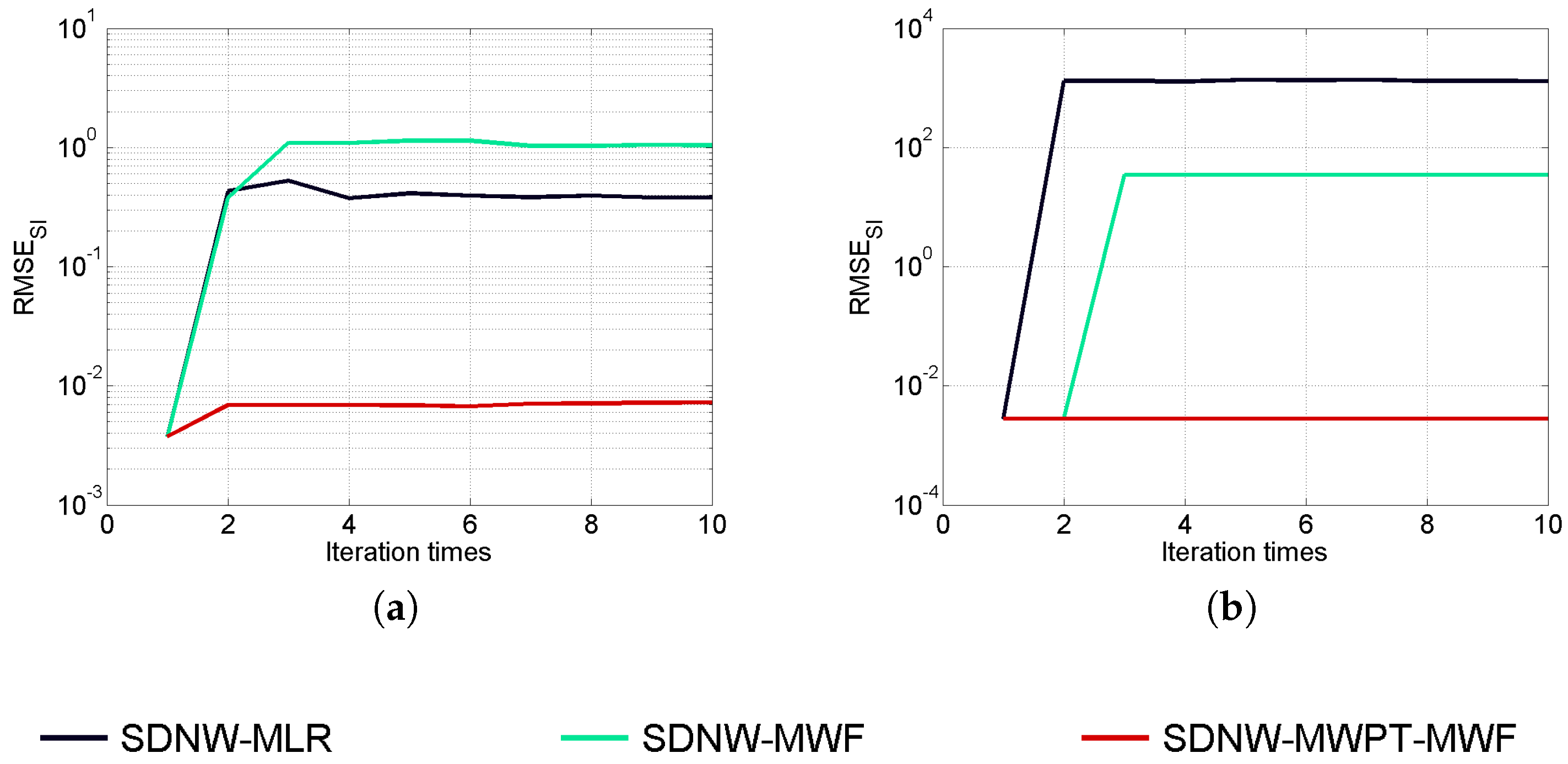
A comparative analysis of SDNW-MWF, SDNW-MLR and SDNW-MWPT-MWF have been carried out by analyzing $RMS{E}_{SD}$ and $RMS{E}_{SI}$ with the maximum iteration times being set as 10. Figure 4 and Figure 5 present the evolution of $RMS{E}_{SD}$ and $RMS{E}_{SI}$ (in logarithmic scale) with the iteration times. From these two figures, it can be seen that, in the case where $SN{R}_{INPUT}=20$ dB, SDNW-MLR performs better than SDNW-MWF in estimating both ${\sigma }_{u,i_3}^2$ and ${\sigma }_{t,i_3}^2$. However, in the case where $SN{R}_{INPUT}=40$ dB, SDNW-MWF outperforms SDNW-MLR. Nonetheless, in both cases, the proposed SDNW-MWPT-MWF can improve the estimation performance significantly according to the lowest $RMS{E}_{SD}$ and $RMS{E}_{SI}$ it obtains. Moreover, $RMS{E}_{SD}$ and $RMS{E}_{SI}$ are greater than the initial error in SDNW-MLR and SDNW-MWF, whereas $RMS{E}_{SD}$ and $RMS{E}_{SI}$ are well constrained in SDNW-MWPT-MWF.

Figure 4. Evolution of $RMS{E}_{SD}$ with iteration times according to different values of $SN{R}_{INPUT}$: (a) 20 dB; (b) 40 dB.

Figure 5. Evolution of $RMS{E}_{SI}$ with iteration times according to different values of $SN{R}_{INPUT}$: (a) 20 dB; (b) 40 dB.

Apart from ${\sigma }_{u,i_3}^2$ and ${\sigma }_{t,i_3}^2$, the estimate of the signal also influences the accuracy of the noise variance estimate of a pixel (see Equation (10)). Since the post-estimate ${\widehat{x}}_{i_1{i}_2{i}_3}$ of current PWP iteration is used as the pre-estimate ${\tilde{x}}_{i_1{i}_2{i}_3}$ of the next PWP iteration, we only analyze the estimation performance of the post-estimate ${\widehat{x}}_{i_1{i}_2{i}_3}$. To assess the performance of the signal estimator ${\widehat{x}}_{i_1{i}_2{i}_3}$, we resort to the $SN{R}_{INPUT}$, which will be presented in Section 4.2.

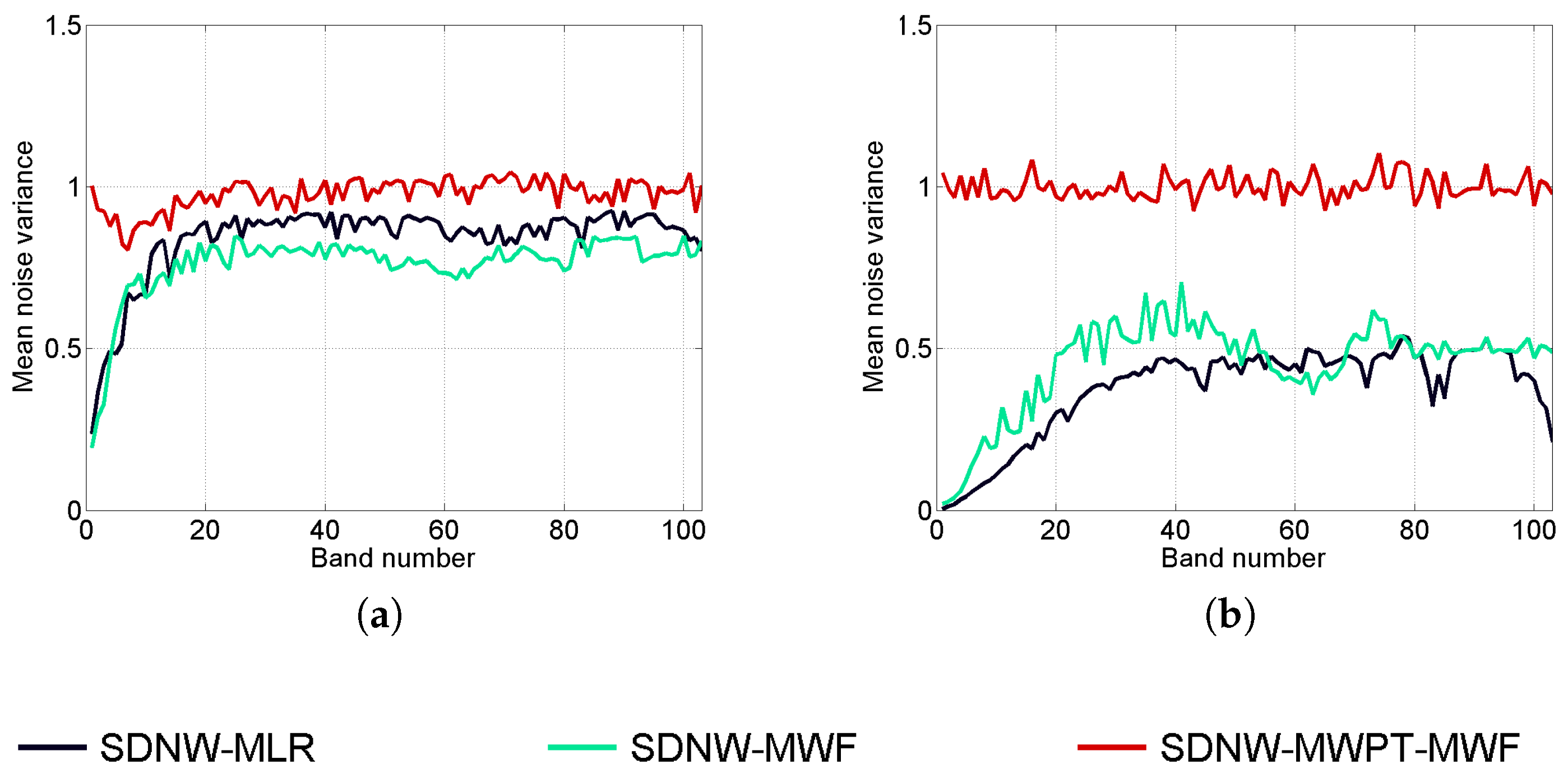
To intuitively present the noise whitening results, Figure 6 shows the mean noise variance of each band after the noise whitening operation. It is evident that the mean noise variance generated by SDNW-MWPT-MWF changes slightly around 1 and is quite constant with respect to the band number. However, the mean noise variance generated by SDNW-MLR and SDNW-MWF is not very satisfactory. In Figure 6a, it can be seen that the trend of the mean noise variances in the lower bands is similar to that in Figure 3 thus implying that the noise in the lower bands (from 1 to 20) is not well whitened. On the other hand, in the bands from 20 to 100, the noise variances are relatively constant, the mean noise variance value is not 1. In Figure 6b, the noise whitening results by SDNW-MLR and SDNW-MWF are worse than that in Figure 6a. Hence, the whitening results in Figure 6 are strongly in favor of the proposed method SDNW-MWPT-MWF.

Figure 6. Curves of noise variance versus band number with $SN{R}_{INPUT}$: (a) 20 dB; (b) 40 dB.

The normal probability plot is usually used to visually ascertain whether or not a dataset is approximately normally distributed, which means that the values in the dataset have the same noise variance. Hence, we supply the normal probability plots of the noise before and after whitening in Figure 7. It is obvious that the noise before whitening (Figure 7a) is not normally distributed. After whitening by SDNW-MWF (Figure 7b), the noise approaches towards the normal distribution though there still remain some values not well whitened as can be observed in the interval [−5, 0]. Nonetheless, the noise values after whitening by SDNW-MLR (Figure 7c) and SDNW-MWPT-MWF (Figure 7d) form a straight line and as such they can be considered as normally distributed. Correspondingly, Figure 8a presents the noise distribution situation in the noise environment where $SN{R}_{INPUT}=40$ dB. It can be seen that the noise values after whitening by SDNW-MLR (Figure 8b) and SDNW-MWF (Figure 8c) are still not normally distributed, while the noise values after whitening by SDNW-MWPT-MWF (Figure 8d) are well normally distributed. The results in Figure 7 and Figure 8 validate once again that the proposed SDNW-MWPT-MWF performs well in both lower ($SN{R}_{INPUT}=20$ dB) and higher ($SN{R}_{INPUT}=40$ dB) SNR noise environments.

Figure 7. Normal probability plot for the noise: (a) before whitening, and whitening after (b) SDNW-MWF; (c) SDNW-MLR; (d) SDNW-MWPT-MWF, with $SN{R}_{INPUT}=20$ dB.

Figure 8. Normal probability plot for the noise: (a) before whitening, and after whitening using (b) SDNW-MLR; (c) SDNW-MWF; (d) SDNW-MWPT-MWF, with $SN{R}_{INPUT}=40$ dB.

4.2. Denoising Performance

In Section 4.1, we have discussed in detail the SD and SI noise variance estimates $RMS{E}_{SD}$ and $RMS{E}_{SI}$. In this subsection, we show some results about the denoising performance. Figure 9 presents the noise removed in band 10 from the ROSIS HSI by SDNW-MLR, SDNW-MWF and SDNW-MWPT-MWF in the noise environment where $SN{R}_{INPUT}=20$ dB. It is obvious that the removed noise is SD noise by comparing visually Figure 9 with the original image Figure 2a. The experimental results in Figure 9 imply that the proposed denoising framework is efficient in removing the SD photon noise in the HSI.

Figure 9. Noise removal using: (a) SDNW-MLR; (b) SDNW-MWF; (c) SDNW-MWPT-MWF, band 10, $SN{R}_{INPUT}=20$ dB.

Additionally, we have assessed the denoising performance of various methods by analyzing the criterion $SN{R}_{OUTPUT}$. Figure 10 presents the evolution of the $SN{R}_{OUTPUT}$ in various noisy environments. It is obvious that the $SN{R}_{OUTPUT}$ generated by SDNW-MWPT-MWF reaches a higher stable value after several iterations. Conversely, the $SN{R}_{OUTPUT}$ of SDNW-MLR and SDNW-MWF are relatively lower than that of SDNW-MWPT-MWF due to the highest estimation errors of $RMS{E}_{SD}$ and $RMS{E}_{SI}$ as shown in Figure 4 and Figure 5, respectively. When $SN{R}_{INPUT}=20$ dB, the $SN{R}_{OUTPUT}$ generated by SDNW-MWF is only improved marginally compared to the $SN{R}_{INPUT}$. On the other hand, when $SN{R}_{INPUT}=40$ dB SDNW-MWF improves the SNR significantly but the $SN{R}_{OUTPUT}$ is not stable in the evolution when the iterations are increased. The SDNW-MLR performs well when $SN{R}_{INPUT}=20$ dB, but when $SN{R}_{INPUT}=40$ dB the denoising performance of SDNW-MLR is not good compared to that of SDNW-MWF and SDNW-MWPT-MWF. This trend becomes worse as the $SN{R}_{OUTPUT}$ of SDNW-MLR is lower than the $SN{R}_{INPUT}$. Moreover, Figure 11 compares the $SN{R}_{OUTPUT}$ of each method from 20 dB to 40 dB with a step of 5 dB. It shows that SDNW-MLR can improve the SNR from 20 to 30 dB, while degrading the SNR from 35 to 40 dB. The SDNW-MWF is even worse as there is only a marginal improvement of the SNR in 20 dB. From 25 to 40 dB, it degrades the SNR. Nonetheless, from the results presented in Figure 10 and Figure 11, we can conclude that SDNW-MWPT-MWF is a stable and reliable denoising method in various noisy environments.

Figure 10. Evolution of $SN{R}_{OUTPUT}$ with iteration times according to different values of $SN{R}_{INPUT}$: (a) 20 dB; (b) 40 dB.

Figure 11. Comparison of denoising results based on $SN{R}_{OUTPUT}$ versus $SN{R}_{INPUT}$.

4.3. Classification after Denoising

In Section 4.2, we have mainly compared various methods with the capability of improving the SNR. However, some methods might also modify the useful signal severely in the denoising process and which cannot be reflected by the SNR. The classification is employed to distinguish different materials in HSIs [21], and it is sensitive to the signal distortion. Hence, in this paper, we take into account the classification improvement ability of the various methods considered.

Two real-world images are considered for this investigation. The first one, referred to as ROSIS HSI, is described in the beginning of this section.

In the ROSIS HSI, there are nine classes: bitumen, self-blocking bricks, trees, shadows, gravel, bare soil, asphalt, painted metal sheets, and meadows, which are shown in Figure 2b and in the ground truth in Figure 12 with different colors. A proportion of $10\%$ of the reference data of each class is randomly selected as the training samples. The numbers of training and testing samples are shown in Table 1. The SVM classifier is employed to do the classification and its kernel function is RBF with $\gamma =1$ and the penalty parameter $C=100$.

Figure 12. Classification reference data:(a) ground truth of the area; (b) nine classes in ROSIS HSI.

Table 1. Training and testing samples used in the classification.

ID	Class	Training Samples	Testing Samples
1	Bitumen	133	1330
2	Self-Blocking Bricks	171	1709
3	Trees	70	697
4	Shadows	49	486
5	Gravel	93	929
6	Bare Soil	503	5029
7	Asphalt	187	1868
8	Painted metal sheets	135	1345
9	Meadows	201	2005
	Total	1542	15,398

The second one, referred to as HYDICE HSI, was acquired by the HYperspectral Digital Imagery Collection Experiment (HYDICE) and has 148 spectral bands (from 435 to 2326 nm), 310 rows, and 220 columns. The scene is shown in Figure 13a. This HSI is modeled as a tensor $\mathbf{R}\in {\mathbb{R}}^{310\times 220\times 148}$ and its ground truth is shown in Figure 13b. According to the ground truth, there are seven land cover classes in HYDICE HSI: field, trees, road, shadow and three different targets. A proportion of $30\%$ of the reference data of each class is randomly selected as the training samples. The numbers of training and testing samples are shown in Table 2.

Figure 13. HSI images: (a) ground truth; (b) classes in HYDICE HSI.

Table 2. Training and testing samples used in the classification.

ID	Class	Training Samples	Testing Samples	Color
1	Field	12,174	40,811	Green
2	Trees	1361	5537	Sea green
3	Road	1146	3226	White
4	Shadow	1363	5036	Maroon
5	Target 1	138	519	Red
6	Target 2	78	285	Blue
7	Target 3	67	223	Yellow
	Total	16,327	55,637

The classification is applied to the denoised HSIs using various methods in order to compare their abilities of improving the classification performance. Figure 14 presents the classification results obtained in the noisy environment where $SN{R}_{INPUT}=30$ dB. It can be seen from the “bare soil” class that there are less misclassified pixels in the results obtained by SDNW-MWPT-MWF compared to the other results. To make it easy to compare, we give the Overall Accuracy (OA) and Kappa coefficient (K) results for the various methods used in Table 3. It can be seen that if the classification is applied directly to the noisy HSI, the OA is only $91.33\%$ and K = $0.71$. After denoising by SDNW-MLR, there is a marginal improvement of OA resulting in $91.88\%$ and K = $0.81$. SDNW-MWF performs better than SDNW-MLR, and its OA is increased to $94.20\%$ and K to $0.94$. The proposed SDNW-MWPT-MWF makes the most significant improvement among the denoising methods. Indeed, its OA is $98.51\%$ and its K is $0.97$. The classification result clearly shows that the proposed SDNW-MWT-MWF is efficient in improving the classification performance.

Figure 14. Classification results of the ROSIS HSI after denoising by: (a) SDNW-MLR; (b) SDNW-MWF; and (c) SDNW-MWPT-MWF. The classification result without denoising (d) is supplied as a benchmark. ($SN{R}_{INPUT}=30$ dB).

Table 3. OA (%) and Kappa of the classification of the denoised ROSIS HSI, $SN{R}_{INPUT}=30$ dB.

Methods	Without Denoising	SDNW-MLR	SDNW-MWF	SDNW-MWPT-MWF
OA	91.33	91.88	94.20	98.51
Improvement	0	0.55	2.87	7.18
Kappa	0.79	0.81	0.91	0.96
Improvement	0	0.02	0.12	0.17

To investigate how the number of training samples affects the performance of our method and other comparison methods, we considered a proportion of $50\%$ of the reference data of each class is randomly selected as the training samples. Table 4 shows the OA and Kappa coefficient results. As shown from Table 3 and Table 4, our proposed method outperforms all other methods. In particular, with the number of training samples reducing ($10\%$), our method could obtain bigger accuracy gains than other comparison methods.

Table 4. OA (%) and Kappa of the classification of the denoised ROSIS HSI, $SN{R}_{INPUT}=30$ dB.

Methods	Without Denoising	SDNW-MLR	SDNW-MWF	SDNW-MWPT-MWF
OA	91.98	92.73	95.92	99.06
Improvement	0	0.75	3.94	7.08
Kappa	0.81	0.84	0.94	0.98
Improvement	0	0.03	0.13	0.16

Figure 15 shows the OA values obtained from the denoised HYDICE HSI and shows that the SDNW-MWPT-MWF method permits reduction of the noise, which is of great interest for SVM classifier. The comparison of the OA and Kappa values (see Table 5) calculated for each preprocessing of denoising shows that the multilinear algebra-based method SDNW-MWPT-MWF leads to better classification results than the considered methods in this experiment.

Figure 15. Classification results of the HYDICE HSI after denoising by: (a) SDNW-MLR; (b) SDNW-MWF; and (c) SDNW-MWPT-MWF. The classification result without denoising (d) is supplied as a benchmark. ($SN{R}_{INPUT}=30$ dB).

Table 5. OA (%) and Kappa of the classification of the denoised HYDICE HSI, $SN{R}_{INPUT}=30$ dB.

Methods	Without Denoising	SDNW-MLR	SDNW-MWF	SDNW-MWPT-MWF
OA	95.60	95.66	97.22	99.94
Improvement	0	0.06	1.62	4.34
Kappa	0.894	0.895	0.945	0.989
Improvement	0	0.01	0.51	0.95

To make the experimental results more convincing, we have compared the classification improvement performance of SDNW-MLR, SDNW-MWF and SDNW-MWPT-MWF in varying noisy environments, i.e., $SN{R}_{INPUT}$ varies from 20 dB to 40 dB with a step of 5 dB. The classification result of the noisy HSI without denoising is also supplied as a benchmark. Figure 16 presents the curves of OA versus $SN{R}_{INPUT}$. In the cases where the HSI is impaired severely ($SN{R}_{INPUT}=20\mathrm{and}25$ dB), the classification result can be improved significantly after denoising, which implies that the denoising is a necessary preprocessing procedure prior to the classification. Above 30 dB, SDNW-MLR can only improve the classification result marginally and the same is valid for SDNW-MWF with more than 35 dB. Nonetheless, SDNW-MWPT-MWF performs better than SDNW-MLR and SDNW-MWF and it improves the OA significantly for $SN{R}_{INPUT}$ values from 20 dB to 40 dB.

Figure 16. Classification OA with respect to $SN{R}_{INPUT}$.

5. Discussion

Hyperspectral sensors collect data in hundreds of narrow contiguous spectral bands, providing a powerful means to discriminate different materials by their spectral features. In the last decade, for improving the classification, several denoising algorithms for hyperspectral images were proposed. Most were derived assuming the spatial stationarity of the noise that affects hyperspectral images, meaning that the noise characteristics are assumed to be the same in each hyperspectral image region. The existing algorithms are proposed to remove the signal independent noise for enhancing hyperspectral image applications. In this study, we have proved that assumption is not valid for new-generation hyperspectral sensors, where photon noise, which depends on the spatially varying signal level, is not negligible. We are thus studying the possible impacts of signal-dependent noise on the performance of existing classification algorithms. By assuming a signal-dependent noise model, we have proposed a novel multilinear algebra-based algorithm to remove simultaneously the signal-independent noise and signal-dependent noise. This result has inspired a new iterative procedure noise-whitening (SDNW-MWPT-MWF) which improves the SVM’s robustness in the presence of signal-dependent noise. The noise-whitening is achieved by exploiting estimates of the noise variance for each band and for each pixel. The performance of the proposed SDNW-MWPT-MWF method are validated on the simulated HSIs disturbed by both SD and SI noise and on the real-world ROSIS and HYDICE HSIs. From the analysis and the comparative study against other similar methods in the experiments, it can be concluded that SDNW-MWPT-MWF method can effectively reduce both SD and SI noise from HSIs. It is also necessary to take into account the signal-dependent noise in the denoising when dealing with HSIs that were collected by a new-generation airborne hyperspectral sensors. Indeed, this study demonstrated that the signal-dependent noise may affect the properties of existing classification algorithms, thus encouraging future work about the impact of SD noise. Our ongoing activity is aimed at demonstrating the benefits arising from using the SDNW-MWPT-MWF algorithm in mitigating the impact of the SD noise in different algorithms for hyperspectral data exploitation.

Since in this study the optimal parameter combination is found by time-consuming brute force searching, future works will be focused on the reduction of the computational load. A heuristic algorithm can be used to search for the optimal (sub-optimal) parameter combination such as a genetic algorithm.

6. Conclusions

In this paper, a denoising method SDNW-MWPT-MWF has been proposed under the PWP denoising framework for the purpose of reducing the SD photon and SI thermal noise in HSIs. Two other adapted denoising methods SDNW-MLR, SDNW-MWF are also used as comparative methods. The performances of these methods are compared in the case of photon noise whitening, denoising and improvement of classification. The photon noise whitening experiment, the denoising experiment and the classification experiment are designed to assess the parameter estimation performance, the improvement of the SNR and the distortion of the spectra in the HSI, respectively. From the experimental results obtained, it can be concluded that the SDNW-MLR performs well in removing the noise, though it also changes the signal severely in the denoising process as shown from the lower classification result OA. In contrast, SDNW-MWF performs well in preserving the signal though it cannot remove the noise well from the images. However, the proposed SDNW-MWPT-MWF is able to obtain high $SN{R}_{OUTPUT}$ as well as the high OA, thus implying that it is able to remove noise well while still preserving the signal.

These promising results encourage us to extend our experiments on other hyperspectral data such as Indian Pines and Salinas HSIs.

In this study, we employed the HYNPE algorithm to estimate the noise parameters, and then filtered noise by the proposed method SDNW-MWPT-MWF. Nonetheless, SDNW-MWPT-MWF converts SD noise to additive white Gaussian noise by a pre-whitening procedure and then applied MWPT-MWF. Due to the parameter estimate errors, the whitened noise is only approximately white, therefore the performance of filters developed for the white noise might degrade. Thus, it is interesting to develop a filter that can directly process the SD noise without the noise whitening procedure. For example, the tensor-based filtering method using a PARAFAC tensor decomposition could be carried out in the future.

Appendix A.1. Definition of a Tensor

An N-th order tensor is an N-dimensional array, $\mathcal{X}\in {\mathbb{R}}^{I_1\times \dots \times I_N}$, in which $\mathbb{R}$ indicates the real manifold, and N is the number of dimensions. The elements in this tensor can be expressed as $x_{i_1\dots i_N}$, with $i_1=1,\dots ,I_1;\cdots ;i_N=1,\dots ,I_N$. The nth dimension of this tensor is called mode-n.

Appendix A.2. Unfolding

Unfolding is also known as matricization or flattening. It can convert a tensor into its matrix form for the conveniency of using matrix-based data analyzing methods. A tensor can be unfolded in different ways according to the mode in which the unfolding is performed. The unfolding in mode-n is called mode-n unfolding.

Let ${\mathbf{X}}_n\in {\mathbb{R}}^{I_n\times M_n}$ denote the mode-n unfolding matrix of a tensor $\mathcal{X}\in {\mathbb{R}}^{I_1\times \dots \times I_N}$, where $M_n=I_{n+1}{I}_{n+2}\dots I_N{I}_1\dots I_{n-1}$. The columns of ${\mathbf{X}}_n$ are the $I_n$-dimensional vectors obtained from $\mathcal{X}$ by varying index $i_n$ while keeping the other indices fixed.

Appendix A.3. Mode-n Tensor Product × n

The mode-n product is defined as the product between a data tensor $\mathcal{X}\in {\mathbb{R}}^{I_1\times \dots \times I_N}$ and a matrix $\mathbb{B}\in {\mathbb{R}}^{J\times I_n}$ in mode n. This mode-n product is denoted by $\mathcal{C}=\mathcal{X}{\times }_n\mathbb{B}$, whose entries are given by

$$c_{i_1\dots i_{n-1}j{i}_{n+1}\dots i_N}\triangleq \sum _{i_n=1}^{I_n}{x}_{i_1\dots i_{n-1}{i}_n{i}_{n+1}\dots i_N}{b}_{j{i}_n},$$

(A1)

where $\mathcal{C}\in {\mathbb{R}}^{I_1\times \dots \times I_{n-1}\times J\times I_{n+1}\times \dots \times I_N}$.

Appendix A.4. Element Extraction

For a given tensor $\mathcal{X}\in {\mathbb{R}}^{I_1\times I_2\times \dots \times I_N}$, we define the following element extraction operation:

$$\mathcal{X}(i_1,i_2,\dots ,i_N)\triangleq x_{i_1{i}_2\dots i_N}.$$

(A2)

Appendix A.5. Hadamard Product ⊛

The Hadamard product is defined as the product of two equal-size tensors $\mathcal{X}\in {\mathbb{R}}^{I_1\times I_2\times \dots \times I_N}$ and $\mathcal{Y}\in {\mathbb{R}}^{I_1\times I_2\times \dots \times I_N}$. The entries of the Hadamard product $\mathcal{Z}=\mathcal{X}⊛\mathcal{Y}$ can be computed as:

$$z_{i_1\dots i_{n-1}{i}_n{i}_{n+1}\dots i_N}=x_{i_1\dots i_{n-1}{i}_n{i}_{n+1}\dots i_N}{y}_{i_1\dots i_{n-1}{i}_n{i}_{n+1}\dots i_N},$$

(A3)

where $\mathcal{Z}\in {\mathbb{R}}^{I_1\times I_2\times \dots \times I_N}$.

Appendix A.6. Mode-n Rank of a Tensor

The term mode-n rank $K_n$ of a tensor $\mathcal{X}\in {\mathbb{R}}^{I_1\times I_2\times \dots \times I_N}$, denoted by $K_n={\mathrm{rank}}_n\left(\mathcal{X}\right)$, is the dimension of the column space of the mode-n unfolding matrix ${\mathbf{X}}_n$ [29], i.e.,

$$K_n={\mathrm{rank}}_n\left(\mathcal{X}\right)=\mathrm{rank}\left({\mathbf{X}}_n\right).$$

(A4)

The term mode-n rank is another way to extend the notion of the matrix rank to the tensor case. The mode-n rank is actually a rank of a matrix, therefore it can be analyzed by using matrix based techniques. Nevertheless, for a matrix $\mathbf{X}$, the ranks of its column space and row space are similar, $\mathrm{rank}\left(\mathbf{X}\right)=\mathrm{rank}\left({\mathbf{X}}^T\right)$, but, for the tensor $\mathcal{X}$, the different mode-n ranks are not necessarily the same. This means that the mode-n rank of tensor $\mathcal{X}$ is not a unique value but a set of N values $\left\{K_1,\dots ,K_N\right\}$.

Appendix C.1. MWPT

MWPT can be computed by performing 1D wavelet packet transform in each mode [32]. Therefore, the wavelet packet coefficient tensor ${\mathcal{C}}_{\mathbf{l}}^{\mathcal{R}}$ can be computed as

$${\mathcal{C}}_{\mathbf{l}}^{\mathcal{R}}=\mathcal{R}{\times }_1{\tilde{\mathbf{W}}}_1^{l_1}{\times }_2{\tilde{\mathbf{W}}}_2^{l_2}{\times }_3{\tilde{\mathbf{W}}}_3^{l_3},$$

(A14)

and the reconstruction can be written as

$$\mathcal{R}={\mathcal{C}}_{\mathbf{l}}^{\mathcal{R}}{\times }_1{\left({\tilde{\mathbf{W}}}_1^{l_1}\right)}^T{\times }_2{\left({\tilde{\mathbf{W}}}_2^{l_2}\right)}^T{\times }_3{\left({\tilde{\mathbf{W}}}_3^{l_3}\right)}^T,$$

(A15)

where $\mathbf{l}={[l_1,l_2,l_3]}^T$, and $l_1,l_2,l_3\ge 0$. In particular, when $l_1,l_2,l_3>0$, MWPT indicates the 3D wavelet packet transform. ${\tilde{\mathbf{W}}}_k^{l_k}$ denotes the $l_k$ level wavelet packet transform to kth mode of $\mathcal{R}$. ${\mathcal{C}}_{\mathbf{l},\mathbf{m}}^{\mathcal{R}}$ is defined as the coefficient subtensor of ${\mathcal{C}}_{\mathbf{l}}^{\mathcal{R}}$, where $\mathbf{m}={[m_1,m_2,m_3]}^T$ is the index vector, and $0\le m_k\le 2^{l_k}-1$, $k=1,2,3$. Then, for each element of ${\mathcal{C}}_{\mathbf{l},\mathbf{m}}^{\mathcal{R}}$, we can define:

$${\mathcal{C}}_{\mathbf{l},\mathbf{m}}^{\mathcal{R}}(j_1,j_2,j_3)\triangleq {\mathcal{C}}_{\mathbf{i}}^{\mathcal{R}}({\mathbf{J}}_1\left(j_1\right),{\mathbf{J}}_2\left(j_2\right),{\mathbf{J}}_3\left(j_3\right)),$$

(A16)

where

$$\left\{{\mathbf{J}}_n={\left[\frac{m_n{I}_n}{2^l},\dots ,\frac{(m_n+1)I_n}{2^l}-1\right]}^T,n=1,2,3\right\}$$

(A17)

and

$$j_n\in \left\{1,\dots ,\frac{I_n}{2^l}\right\},n=1,2,3.$$

(A18)

The notation ${\mathcal{C}}_{\mathbf{l},\mathbf{m}}^{\mathcal{R}}(j_1,j_2,j_3)$ indicates the element of tensor ${\mathcal{C}}_{\mathbf{l},\mathbf{m}}^{\mathcal{R}}$ in position $(j_1,j_2,j_3)$ as defined in Equation (A2). From the properties of the wavelet packet transform, we know that $m_n$ indicates the “frequency” of mode n. Thus, $\mathbf{m}$ is the frequency index of coefficient block ${\mathcal{C}}_{\mathbf{l},\mathbf{m}}^{\mathcal{R}}$. For convenience, a component tensor of $\mathcal{R}$ is referred to as ${\mathcal{C}}_{\mathbf{l},\mathbf{m}}^{\mathcal{R}}$ in this paper.

Appendix C.2. Multiway Wiener Filter in Multidimensional Wavelet Packet Domain

In the existing MWF algorithm, the filter is applied to the whole hyperspectral image $\mathcal{R}$. As the calculation of the filters needs the estimation of the signal subspace or rank in each mode for suppressing the smallest eigenvalues [33], some weak signal might be removed in this procedure. Therefore, the SNR is an important factor influencing the rank. When SNR is higher, the rank estimated is greater, therefore more signal is preserved in the filtering process. In the contrast condition, more signal is lost. When the noise is white, the power of noise in each component ${\mathcal{C}}_{\mathbf{l},\mathbf{m}}^{\mathcal{R}}$ is the same, whereas the signal concentrates in the lower frequency component. That is to say, in different components, the SNR is different. When MWF is applied to each component, more signal can be preserved. Performing MWPT to tensor $\mathcal{R}$, $\mathcal{X}$ and $\mathcal{N}$ in Equation (1), we obtain:

$$\begin{array}{c}\mathcal{R}{\times }_1{\tilde{\mathbf{W}}}_1^{l_1}{\times }_2{\tilde{\mathbf{W}}}_2^{l_2}{\times }_3{\tilde{\mathbf{W}}}_3^{l_3}\hfill \\ =\left(\mathcal{X}+\mathcal{N}\right){\times }_1{\tilde{\mathbf{W}}}_1^{l_1}{\times }_2{\tilde{\mathbf{W}}}_2^{l_2}{\times }_3{\tilde{\mathbf{W}}}_3^{l_3}\hfill \\ =\mathcal{X}{\times }_1{\tilde{\mathbf{W}}}_1^{l_1}{\times }_2{\tilde{\mathbf{W}}}_2^{l_2}{\times }_3{\tilde{\mathbf{W}}}_3^{l_3}+\mathcal{N}{\times }_1{\tilde{\mathbf{W}}}_1^{l_1}{\times }_2{\tilde{\mathbf{W}}}_2^{l_2}{\times }_3{\tilde{\mathbf{W}}}_3^{l_3}.\hfill \end{array}$$

(A19)

The coefficient tensor of each part

$$\begin{array}{cc}\hfill {\mathcal{C}}_{\mathbf{l}}^{\mathcal{R}}& =\mathcal{R}{\times }_1{\tilde{\mathbf{W}}}_1^{l_1}{\times }_2{\tilde{\mathbf{W}}}_2^{l_2}{\times }_3{\tilde{\mathbf{W}}}_3^{l_3},\end{array}$$

(A20)

$$\begin{array}{cc}\hfill {\mathcal{C}}_{\mathbf{l}}^{\mathcal{X}}& =\mathcal{X}{\times }_1{\tilde{\mathbf{W}}}_1^{l_1}{\times }_2{\tilde{\mathbf{W}}}_2^{l_2}{\times }_3{\tilde{\mathbf{W}}}_3^{l_3},\end{array}$$

(A21)

$$\begin{array}{cc}\hfill {\mathcal{C}}_{\mathbf{l}}^{\mathcal{N}}& =\mathcal{N}{\times }_1{\tilde{\mathbf{W}}}_1^{l_1}{\times }_2{\tilde{\mathbf{W}}}_2^{l_2}{\times }_3{\tilde{\mathbf{W}}}_3^{l_3},\end{array}$$

(A22)

and the coefficient tensor of the estimate $\widehat{\mathcal{X}}$:

$${\widehat{\mathcal{C}}}_{\mathbf{l}}^{\mathcal{X}}=\widehat{\mathcal{X}}{\times }_1{\tilde{\mathbf{W}}}_1^{l_1}{\times }_2{\tilde{\mathbf{W}}}_2^{l_2}{\times }_3{\tilde{\mathbf{W}}}_3^{l_3}.$$

(A23)

Extracting the components of each frequency ${\mathcal{C}}_{\mathbf{l},\mathbf{m}}^{\mathcal{R}}$, ${\mathcal{C}}_{\mathbf{l},\mathbf{m}}^{\mathcal{X}}$ and ${\mathcal{C}}_{\mathbf{l},\mathbf{m}}^{\mathcal{N}}$ from ${\mathcal{C}}_{\mathbf{l}}^{\mathcal{R}}$, ${\mathcal{C}}_{\mathbf{l}}^{\mathcal{X}}$ and ${\mathcal{C}}_{\mathbf{l}}^{\mathcal{N}}$ respectively by using Equation (A16), we obtain:

$${\mathcal{C}}_{\mathbf{l},\mathbf{m}}^{\mathcal{R}}={\mathcal{C}}_{\mathbf{l},\mathbf{m}}^{\mathcal{X}}+{\mathcal{C}}_{\mathbf{l},\mathbf{m}}^{\mathcal{N}}.$$

(A24)

From Parseval’s theorem, the following expression can be obtained:

$$\begin{array}{c}\hfill \parallel \mathcal{X}-\widehat{\mathcal{X}}{\parallel }^2=\parallel {\mathcal{C}}_{\mathbf{l}}^{\mathcal{X}}-{\widehat{\mathcal{C}}}_{\mathbf{l}}^{\mathcal{X}}{\parallel }^2=\sum _{\mathbf{m}}{\parallel {\mathcal{C}}_{\mathbf{l},\mathbf{m}}^{\mathcal{X}}-{\widehat{\mathcal{C}}}_{\mathbf{l},\mathbf{m}}^{\mathcal{X}}\parallel }^2,\end{array}$$

(A25)

which means that minimizing the MSE between $\mathcal{X}$ and its estimate $\widehat{\mathcal{X}}$ is equivalent to minimizing the MSE between ${\mathcal{C}}_{\mathbf{l},\mathbf{m}}^{\mathcal{X}}$ and ${\widehat{\mathcal{C}}}_{\mathbf{l},\mathbf{m}}^{\mathcal{X}}$ for each $\mathbf{m}$. If ${\widehat{\mathcal{C}}}_{\mathbf{l},\mathbf{m}}^{\mathcal{X}}$ is estimated by Tucker3 decomposition of ${\mathcal{C}}_{\mathbf{l},\mathbf{m}}^{\mathcal{R}}$:

$${\widehat{\mathcal{C}}}_{\mathbf{l},\mathbf{m}}^{\mathcal{X}}={\mathcal{C}}_{\mathbf{l},\mathbf{m}}^{\mathcal{R}}{\times }_1{\mathbf{H}}_{1,\mathbf{m}}{\times }_2{\mathbf{H}}_{2,\mathbf{m}}{\times }_3{\mathbf{H}}_{3,\mathbf{m}},$$

(A26)

then ${\mathbf{H}}_{1,\mathbf{m}},{\mathbf{H}}_{2,\mathbf{m}},{\mathbf{H}}_{3,\mathbf{m}}$ are the mode-n filters of the multiway Wiener filter [33]. After estimating ${\widehat{\mathcal{C}}}_{\mathbf{l},\mathbf{m}}^{\mathcal{X}}$ for each $\mathbf{m}$, we obtain ${\widehat{\mathcal{C}}}_{\mathbf{l}}^{\mathcal{X}}$ by concatenating ${\widehat{\mathcal{C}}}_{\mathbf{l},\mathbf{m}}^{\mathcal{X}}$. Furthermore, the estimate $\widehat{\mathcal{X}}$ can be obtained by inverse MWPT, i.e.,

$$\widehat{\mathcal{X}}={\widehat{\mathcal{C}}}_{\mathbf{l}}^{\mathcal{X}}{\times }_1{\left({\tilde{\mathbf{W}}}_1^{l_1}\right)}^T{\times }_2{\left({\tilde{\mathbf{W}}}_2^{l_2}\right)}^T{\times }_3{\left({\tilde{\mathbf{W}}}_3^{l_3}\right)}^T.$$

(A27)

Appendix C.3. Best Transform Level and Basis Selection

In MWPT-MWF algorithm, several parameters should be determined:

• Level of transform: the performance of the algorithm is affected by the level of transform, which depends on the size of tensor $\mathcal{R}$. The maximum level can be calculated by:

  $$N_{L_k}=\lceil {log}_2{I}_k\rceil -5,k=1,2,3,$$

  (A28)

  where $\lceil ·\rceil$ rounds a number upward to its nearest integer, and the constant 5 is reduced from $\lceil {log}_2{I}_k\rceil$ to make sure there are enough elements in each mode so that the transform is meaningful. Then, the set of possible transform levels can be expressed as:

  $$L_k=\{0,1,\cdots ,N_{L_k}\},k=1,2,3,$$

  (A29)

  where $\{·\}$ denotes a set.
• Basis of transform: there are many wavelet bases designed for different cases. For the simplicity of expression, we define:

  $$W=\{{\mathrm{w}}_1,{\mathrm{w}}_2,\cdots ,{\mathrm{w}}_{N_W}\}$$

  (A30)

  to denote the set of possible wavelet bases, where $N_W$ is the number of wavelets in this set.

The best transform level and basis should minimize the MSE or risk $R_c\left(\mathcal{X},\widehat{\mathcal{X}}\right)=\mathrm{E}\left[\parallel \mathcal{X}-\widehat{\mathcal{X}}{\parallel }^2\right]$ [34], whose equivalent form using the coefficients can be expressed as

$$R_c\left(\mathcal{X},\widehat{\mathcal{X}}\right)=\sum _{\mathbf{m}}\mathrm{E}\left[\parallel {\mathcal{C}}_{\mathbf{l},\mathbf{m}}^{\mathcal{X}}-{\widehat{\mathcal{C}}}_{\mathbf{l},\mathbf{m}}^{\mathcal{X}}{\parallel }^2\right].$$

(A31)

Then, the best transform level and basis can be selected by

$$\mathbf{l},w=\underset{l_k\in L_k,w\in W}{argmin}\sum _{\mathbf{m}}\mathrm{E}\left[\parallel {\mathcal{C}}_{\mathbf{l},\mathbf{m}}^{\mathcal{X}}-{\widehat{\mathcal{C}}}_{\mathbf{l},\mathbf{m}}^{\mathcal{X}}{\parallel }^2\right],k=1,2,3.$$

(A32)

As the selection of the optimal $\mathbf{l},w$ depends on $\mathcal{X},$ which is generally unknown, to overcome this drawback, an alternative solution should be found. Denoting by ${\widehat{\mathcal{C}}}_{\mathbf{l},\mathbf{m}}^{\mathcal{X}}\left[d\right]$ the estimate of ${\mathcal{C}}_{\mathbf{l},\mathbf{m}}^{\mathcal{X}}$ at the dth ALS loop and noticing that when $\parallel {\widehat{\mathcal{C}}}_{\mathbf{l},\mathbf{m}}^{\mathcal{X}}\left[d\right]-{\widehat{\mathcal{C}}}_{\mathbf{l},\mathbf{m}}^{\mathcal{X}}{[d-1]\parallel }^2$ is minimized, ${\widehat{\mathcal{C}}}_{\mathbf{l},\mathbf{m}}^{\mathcal{X}}\triangleq {\widehat{\mathcal{C}}}_{\mathbf{l},\mathbf{m}}^{\mathcal{X}}\left[d\right]$ is the optimal estimate of ${\mathcal{C}}_{\mathbf{l},\mathbf{m}}^{\mathcal{X}}$ obtained by MWF, and at the same time $\mathrm{E}\left[\parallel {\mathcal{C}}_{\mathbf{l},\mathbf{m}}^{\mathcal{X}}-{\widehat{\mathcal{C}}}_{\mathbf{l},\mathbf{m}}^{\mathcal{X}}{\parallel }^2\right]$ is minimized. Therefore, Equation (A32) can be replaced by:

$$\mathbf{l},w=\underset{l_k\in L_k,w\in W}{argmin}\widehat{R_c},k=1,2,3,$$

(A33)

where

$$\widehat{R_c}=\sum _{\mathbf{m}}{\parallel {\widehat{\mathcal{C}}}_{\mathbf{l},\mathbf{m}}^{\mathcal{X}}\left[d\right]-{\widehat{\mathcal{C}}}_{\mathbf{l},\mathbf{m}}^{\mathcal{X}}[d-1]\parallel }^2.$$

(A34)

Appendix C.4. Summary of the MWPT-MWF Method

The algorithm MWPT−MWF, can be summarized as presented here.

• Find the optimal $l_1,l_2,l_3\in L$ and $w\in W$. Loop $l_1,l_2,l_3$ and w:

  (a)

  Decompose the data $\mathcal{R}$ by MWPT: ${\mathcal{C}}_{\mathbf{l}}^{\mathcal{R}}=\mathcal{R}{\times }_1{\tilde{\mathbf{W}}}_1^{l_1}{\times }_2{\tilde{\mathbf{W}}}_2^{l_2}{\times }_3{\tilde{\mathbf{W}}}_3^{l_3}$.

  (b)

  Extract component ${\mathcal{C}}_{\mathbf{l},\mathbf{m}}^{\mathcal{R}}$ from ${\mathcal{C}}_{\mathbf{l}}^{\mathcal{R}}$ using Equation (A16), for $\mathbf{m}={[m_1,m_2,m_3]}^T$, where $0\le m_k\le 2^{l_k}-1$, $k=1,2,3$.

  (c)

  Filter component ${\mathcal{C}}_{\mathbf{l},\mathbf{m}}^{\mathcal{R}}$ by MWF: ${\widehat{\mathcal{C}}}_{\mathbf{l},\mathbf{m}}^{\mathcal{X}}={\mathcal{C}}_{\mathbf{l},\mathbf{m}}^{\mathcal{R}}{\times }_1{\mathbf{H}}_{1,\mathbf{m}}{\times }_2{\mathbf{H}}_{2,\mathbf{m}}{\times }_3{\mathbf{H}}_{3,\mathbf{m}}$.

  (d)

  Calculate the risk $\widehat{R_c}$ using Equation (A34). If $\widehat{R_c}$ reaches a fixed threshold, return the optimal $l_1,l_2,l_3,w$ and ${\widehat{\mathcal{C}}}_{\mathbf{l},\mathbf{m}}^{\mathcal{X}}$.

• Concatenate ${\widehat{\mathcal{C}}}_{\mathbf{l},\mathbf{m}}^{\mathcal{X}}$ to obtain ${\mathcal{C}}_{\mathbf{l}}^{\mathcal{X}}$ and perform inverse MWPT: $\widehat{\mathcal{X}}={\widehat{\mathcal{C}}}_{\mathbf{l}}^{\mathcal{X}}{\times }_1{\left({\tilde{\mathbf{W}}}_1^{l_1}\right)}^T{\times }_2{\left({\tilde{\mathbf{W}}}_2^{l_2}\right)}^T{\times }_3{\left({\tilde{\mathbf{W}}}_3^{l_3}\right)}^T$.