Abstract
Plant phenology timings, such as spring green-up and autumn senescence, are essential state information characterizing biological responses and terrestrial carbon cycles. Current efforts for the in situ reflectance measurements are not enough to obtain the exact interpretation of how seasonal spectral signature responds to phenological stages in boreal evergreen needleleaf forests. This study shows the first in situ continuous measurements of canopy scale (overstory + understory) and understory spectral reflectance and vegetation index in an open boreal forest in interior Alaska. Two visible and near infrared spectroradiometer systems were installed at the top of the observation tower and the forest understory, and spectral reflectance measurements were performed in 10 min intervals from early spring to late autumn. We found that canopy scale normalized difference vegetation index (NDVI) varied with the solar zenith angle. On the other hand, NDVI of understory plants was less sensitive to the solar zenith angle. Due to the influence of the solar geometry, the annual maximum canopy NDVI observed in the morning satellite overpass time (10–11 am) shifted to the spring direction compared with the standardized NDVI by the fixed solar zenith angle range (60−70°). We also found that the in situ NDVI time-series had a month-long high NDVI plateau in autumn, which was completely out of photosynthetically active periods when compared with eddy covariance net ecosystem exchange measurements. The result suggests that the onset of an autumn high NDVI plateau is likely to be the end of the growing season. In this way, our spectral measurements can serve as baseline information for the development and validation of satellite-based phenology algorithms in the northern high latitudes.
Keywords:
spectral reflectance; NDVI; in situ; interior Alaska; black spruce; phenology; autumn; net ecosystem exchange 1. Introduction
The rising temperature in the northern high latitudes is abrupt and greater than the global mean [1,2,3]. The Arctic Monitoring and Assessment Programme (AMAP) warned that the temperature increase from 2011 to 2015 was the largest ever recorded [4]. One of the key questions in the Arctic and world communities is how boreal ecosystems respond to such climate and environmental changes. Yet it has not been answered clearly because of difficulties in untying the complex positive and negative feedbacks [5,6,7,8,9]. Amid several key aspects of boreal ecosystems in the context of climate change, plant phenology (e.g., spring green-up, and autumn senescence) is essential state information characterizing the biological response, and even regional and global carbon cycles [10,11,12,13,14,15,16,17].
As first-order information, satellite observation provides geographical information of seasonal spectral reflectance and vegetation indices. Such reflectance information is used to derive plant phenology-like variables by well-established remote sensing algorithms (e.g., NDVI threshold [18], NDVI curve fitting [19], NDII minimum [20]). Here, NDVI is a normalized difference vegetation index as computed by (NIR − Red)/(Red + NIR) and NDII is a normalized difference infrared index as computed by (NIR − SWIR)/(NIR + SWIR). Red, NIR, and SWIR are reflectances in red, near infrared, and shortwave infrared spectral regions, respectively. These phenology-like variables, such as the start of the growing season (SOS) and the end of the growing season (EOS) may or may not be related to actual plant phenology. For example, satellite-derived SOS is greatly affected by the snow melt timing [21,22,23,24]. The previous study suggested that the leaf emergence trend coincided with the snow melt trend in Northern Eurasia [21]. However, there are not enough in situ evidences in the whole boreal forests. Eventually, the accuracy of SOS depends on the degree of synchronism in snow melt and leaf emergence timings.
The autumn phenological variable, EOS, is also a mixture of plant senescence and snow. In addition, recursive cloud appearance impedes a sufficient number of retrievals of surface reflectances, making it difficult to determine EOS timings. Nearly one month biases have been found between satellite EOS and actual plant senescence [22,25]. If the biases between EOS and plant senescence shift together with the same proportion under rising temperatures, satellite EOS could be a representative variable as plant senescence. However, it is highly uncertain whether the senescence timings shift with rising temperatures because some plant species may simply follow photoperiods rather than temperature change [26,27].
Another important fact in boreal forests is that understory plants influence satellite EOS. In evergreen needleleaf forests, the seasonality of tree leaves in terms of their colors and total leaf areas are weak throughout the growing season [28]. The extremely sparse canopy makes the understory bright and thus quite a lot of reflected light from the understory layer goes back in the sensor direction, whereas the contribution pertains to canopy openness and solar/view zenith angles [29]. In other words, understory information can be retrieved by satellite measurements [30,31,32].
Recently, canopy radiative transfer analysis suggested the occurrence of the autumn high plateau in NDVI time-series [22]. This happens potentially because NDVI at the understory senescence period keeps higher levels than during the snow-covered period. The other reason is attributed to the higher solar zenith angle in autumn. As the solar zenith angle is higher, more solar radiation is reflected by the overstory green needles rather than senescent understory plants. NDVI in autumn, thus, contains more overstory information. Yet this phenomenon has not been clearly detected by in situ nor satellite observations.
Current efforts for the in situ reflectance measurements are not enough to obtain the exact interpretation of how seasonal spectral signature responds to phenological stages in boreal evergreen needleleaf forests. Some previous studies have revealed seasonality and the contribution of understory plants to canopy reflectance in north European and Canadian forests though those measurements are rather sporadic to quantify subtle and quick changes in spectral signals ([29,33,34,35]). To quantify the phenology signal, continuous measurements throughout the growing season are necessary.
This study shows the first in situ continuous time-series measurements of spectral reflectance and vegetation index computed by the reflectance measurements in a boreal forest in interior Alaska. We deployed two field-based spectroradiometer systems in an open black spruce forest. These two spectroradiometer systems were used to obtain canopy scale (overstory + understory) and understory reflectances. The objectives of this study were to understand how spectral reflectance responds to growing season phenology. We have three research questions. (1) The first question is how seasonal changes in solar zenith angle affect the spectral reflectance and vegetation index. The seasonal change of spectral signatures is controlled by seasonal changes in black spruce tree and understory species. The seasonal change in solar zenith angle potentially affects the spectral signature because of the change in the shadow area of crowns and trunks, and the seasonal changes in the contribution of reflected radiation from overstory; (2) The second question is how canopy scale and understory spectral signatures differs. Canopy reflectance is influenced by both black spruce and understory plant species. Black spruce is an evergreen needleleaf tree and it has weak seasonality. On the other hands, the majority of understory plants show seasonal changes in leaf area and colors; (3) The last question is how the seasonality in spectral signature correspond to eddy covariance net ecosystem exchanges (NEE). It is truly important to link the satellite signals with biological activities in boreal forests. Ultimately, these spectral data will serve as baseline information for the development of improved satellite phenology algorithms and terrestrial biosphere models.
2. Materials and Methods
2.1. Study Site
The study site, Poker Flat Research Range, referred to as US-Prr in AmeriFlux [36,37], is a sparse evergreen needleleaf forest located in 50 km northeast from Fairbanks, Alaska, USA (65°07′24”N, 147°29′15”W, elevation 210 m a.s.l) [36,38]. CO2 and water fluxes, and meteorological measurements have been performed on a 17-m scaffold tower since 2010. The spectral reflectance measurements have been continued since 2015. The eddy covariance systems were installed at the height of 11 m on the tower and 1.9 m on the tripod located 15 m away from the tower. The site experiences a subarctic climate with cold winters and mild summers. The average daily temperature in February and July were −20.2 °C and 14.6 °C, respectively in 2011–2016. This site is situated on a discontinuous permafrost region. The active layer depth was at 43 cm (the deepest of the year) and soil deeper than 43 cm was permafrost [36].
Black spruce (Picea mariana) is the dominant overstory tree species and the percentage of tree cover across the landscape is less than 20%. Overstory leaf area index (LAI) is 0.73 [39] and the canopy height (A cumulative basal area inflection) is 2.91 m [36]. The stem density of trees higher than 1.3 m is 3967 trees ha−1 [36]. The aboveground biomass around the study site is 12.7 (Mg DW ha−1, [40]). The understory is fully covered with shrubs, sedges, moss, and lichen. Peat moss (Sphagnum fuscum) and feather moss (Hylocomium splendens) are dominant on the understory. Northern reindeer lichen (Cladina stellaris) are also distributed sporadically. Shrubs and sedges, such as Labrador tea (Ledum groenlandicum), bog bilberry (Vaccinium uliginosum), cloudberry (Rubus chamaemorus), bog birch (Betula glandulosa or Betula nana) and cotton grass (Eriophorum vaginatum) as tussock formations are often found at the surface [37]. Snow melt and continuous snow cover occurs in late April to May and in October [14,41], respectively. The leaf emergence of understory plants occurs soon after the snow melt and senescence starts in late August [22,42].
2.2. Spectral Reflectance Measurements and Data Processing
Details of the sensor deployments, data processing and quality control are described in Appendix A and Appendix B. Here, we summarized the outline of the measurements. Two visible and near infrared spectroradiometer systems, MS-700 (Eko Instruments Co., Ltd., Tokyo, Japan) and rotating platforms (Hayasaka Rikoh Co., Ltd., Sapporo, Japan) [43] were installed at the study site in 2015 for the canopy scale and understory reflectance measurements (Figure 1). The location of the spectroradiometers constitutes the typical tree stand conditions around the site. To measure the canopy scale and understory reflectances, one MS-700 sensor was put on the top of the 17-m scaffold tower (Figure 1a) and another MS-700 was installed at 1.5 m height with a tripod situated at approximately 20 m northwest of the tower (Figure 1b). The location of the understory MS-700 system was chosen being included in the field of view of the tower top MS-700 system but sufficiently apart from the scaffold tower to avoid the impact of light reflection and shadow. The measured quantities by the MS-700 systems were hemispherical irradiance (field of view = 180°). The spectral reflectance was quantified as a ratio of surface reflected radiation to incoming sky radiation. As the MS-700 sensor measured hemispherical irradiance, reflectance measurements were directional-hemispherical reflectance in the presence of a solar beam and bi-hemispherical reflectance in thick cloud conditions. Daily spectral reflectance measurements were scheduled from 7 am to 7 pm on Alaska Standard Time (AKST) with an interval of ten minutes.
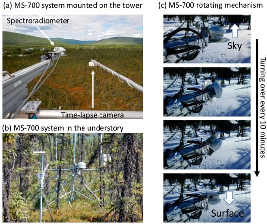
Figure 1.
The field deployment of the spectroradiometer systems. (a) MS-700 system on the top of the scaffold tower. Hemispherical time-lapse camera is located next to the MS-700 system. (b) MS-700 system on the understory layer. (c) MS-700 turning over mechanism. The MS-700 spectroradiometer turns over every 10 min to measure the surface reflected irradiance.
In the current analysis, the observations in 2017 were selected because the year 2017 contains almost a full complement of seasonal data. Because the sky and surface measurements have the four-minute time lag, the computed reflectances were affected by the short-term variations in solar radiation. To remove the erroneous reflectance data, we excluded the data with short-term solar radiation variations (details of the quality control are described in Appendix B). The spectral measurements on the scaffold tower contained the forward reflection from the scaffold structure. We removed the data measured between 12:00–14:00 from our analysis. After removing the erroneous data, the fraction and number of valid data in 2017 were N = 5547 out of 17,370 (33.9%) for the tower top measurements and N = 6717 out of 17,370 (41.0%) for the understory measurements. The spectral reflectances in Red and NIR were computed as close as the spectral ranges of Terra-MODIS band 1 (620–670 nm) and band 2 (841–876 nm), respectively. Although we removed the measurements that were highly affected by the tower reflection, other measurements also contained a residual offset by the tower reflection. We compared the alternate reflectance data measured by the narrower field of view sensor (HR4000, Ocean Optics, Inc., Largo, FL, USA, FOV = 25°, FWHM = 0.2 nm), and Red and NIR reflectances were calibrated. NDVI was computed from Red and NIR reflectances. The seasonal reflectance and NDVI data were divided into five phenological stages: spring snowy stage A: day of year (DOY) 80–100, green-up stage B: 111–125, summer stage C: 126–220, autumn before snow stage D: 221–282, autumn snowy stage E: 283–304 (Figure 2). To evaluate the relative changes in seasonal NDVIs, a normalized NDVI was computed from the annual maximum and minimum NDVI (NDVImax and NDVImin):
Normalized NDVI = (NDVI − NDVImin)/(NDVImax − NDVImin)
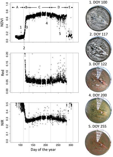
Figure 2.
Seasonal variations in canopy scale normalized difference vegetation index (NDVI), and reflectances in Red and NIR in 2017. All quality-controlled data are shown. A–E indicates the division of phenological stages analyzed in this study. Stage A: Day of the year (DOY) 80–110, stage B: DOY 111–125, stage C: DOY 126–220, stage D: 221–282, and stage E: DOY 283–304. Hemispherical images on the typical phenological timings are also shown in the right side. Vertical dotted gray lines are the date of the time lapse camera images (1: DOY 100, 2: DOY 117, 3: DOY 122, 4: DOY 200, and 5: DOY255).
2.3. Time-Lapse Camera
Time-lapse photography provided the actual status of plant species. Photograph images were used to visually confirm the plant growth stage and snow coverage around the field of spectroradiometer views. We used two time-lapse camera systems. At the tower top (height = 17 m), a time–lapse hemisperhical camera system, consisting of a Nikon (Tokyo, Japan) Coolpix 4500 with an FC-E8 fisheye lens and a Hayasaka Rikoh (Sapporo, Japan) SPC31A controller, took a downward hemispehrical image every 60 min. This camera system was installed in parallel with the spectroradiometer, MS-700 (Figure 1a). The distance between the camera system and spectroradiometer was approximately 1 m. Thus, both systems shared nearly the same field of view. At the understory level, a time-lapse camera system by Rasberry-pi (Raspberry Pi Foundation) was installed on the slide rail of the spectroradiometer. The Rasberry-pi camera system takes nadir-view images every 60 min. Although the field of view of the Rasberry-pi camera system was not completely matched with that of the spectroradiometer, they could capture the same understory plant conditions. The images were provided by the Phenological Eyes Network [44]. They are publicly available at http://www.pheno-eye.org (Site ID: PFA).
2.4. Eddy Covariance Flux Data
Net ecosystem exchange (NEE) was measured by the eddy covariance system installed at 11 m on the scaffold tower in the site (AmeriFlux ID: US-Prr). The 10 Hz CO2 mixing ratio and three-dimensional wind speed were measured by an enclosed infrared gas analyzer (LI-7200, LI-COR, USA). The data were processed by the EddyPro (LI-COR Corporate, USA) and 30 min NEE flux (µmol m−2 s−1) were computed. The details of site installation conditions and data processing were summarized in previous studies [36,37]. The 30 min NEE fluxes were then converted to the daily mean NEE. To remove the short-term NEE variability because of day to day meteorological changes, a five day moving window average was applied to the daily NEE datasets.
3. Results
Figure 2 and Figure A1 in Appendix C show seasonal changes in canopy scale NDVI and corresponding images in 2017. Seasonal NDVI patterns were not a symmetrical shape from spring to summer and from summer to autumn. In spring, a rapid increase in NDVI started in DOY 115 and ended in DOY 122. NDVI gradually increased until DOY 200 and decreased until DOY 255. From DOY 255 to DOY 282, there was an autumn high plateau for 27 days, whereas autumn NDVIs were noisier than other phenological stages. After DOY 282, NDVI abruptly decreased because of snow. The plotted NDVIs had deviations because of differences in observation time. The phenological stage around the autumn NDVI high plateau had the highest deviations throughout the observation period.
3.1. Impact of Solar Zenith Angle to NDVI and Spectral Reflectance
The seasonal changes of spectral signatures and NDVI are controlled by seasonal changes in black spruce tree and understory species. The solar zenith angle could also affect the spectral signature and NDVI. Thus, we evaluated the impact of the solar zenith angle to spectral signatures and NDVI. The observed spectral reflectance and NDVI showed different solar zenith angle (SZA) dependencies between canopy scale and understory measurements, and among the different phenological stages (the NDVI-SZA plots from stage A to E) (Figure 3, Figure A2 and Figure A3 in Appendix D). Circle colors in Figure 3 denote the DOY for each phenology stage with earlier days in reddish to later days in bluish. The plots with the same color indicate the measurements on the same day. In all phenological stages, understory measurements were less dependent on the solar zenith angle (Figure 3 right). Although understory NDVI shows large day by day changes (e.g., Stage B), the same day measurements were on the constant NDVI level. This does not mean the spectral reflectances were also constant through a range of solar zenith angles (Figure A2 and Figure A3): both Red and NIR reflectances exhibit non-linear behavior, particular in stages A and B, whereas reflectances in stages C and D were more stable.
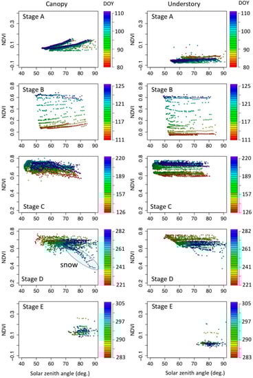
Figure 3.
Solar zenith angle dependency of NDVI in five phenological stages. The definition of phenological stages are shown in Figure 2. Left: Canopy scale NDVI (measured at the top of the tower). Right: Understory measurements. Colors on the plotted circles denote the day of the year (DOY) of the measurements.
In contrast, canopy scale NDVI exhibits either positive or negative slopes against the solar zenith angle (Figure 3 left). This NDVI behavior varies with snow coverages on the understory layer. In stage A, where the understory is fully covered with snow, canopy scale NDVI increases with increased solar zenith angle. Stage B is a transition from positive to negative slope to NDVI–SZA plots. Consistent negative NDVI–SZA slopes were found in stage C. In later periods of stage D (bluish circles in Figure 3 left “stage D”), there were two types of NDVI patterns: the first type was an almost flat NDVI against the solar zenith angle. The other type was the NDVI curve that decreased with solar zenith angle. The later decreasing NDVI curve was the effect of intermittent snow fall in this phenological stage.
Magnitudes of canopy scale NDVI–SZA slopes were all larger than that of understory NDVI–SZA (Figure 4). Note that the slopes for stage D were computed without snow-affected NDVI, and slopes for stage E were not computed because of the limited solar zenith angle ranges. Among the four phenological stages (A to D), the canopy scale NDVI-SZA slopes were highest in stage B (greenup periods, mean = 0.0025), followed by stage A (spring snowy stage, mean = 0.0018). Stage D was the lowest slope (mean = 0.0006), and there are no obvious differences in canopy scale and understory NDVI-SZA slopes.
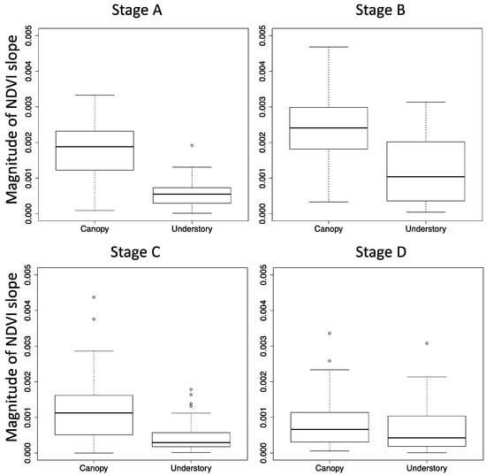
Figure 4.
Boxplot of the NDVI slope in each phenological stage. Magnitude of NDVI slope indicates the absolute value of NDVI slope against solar zenith angle. NDVI values for each day were extracted and the slope was calculated. Stage E was not computed because of limited solar zenith angle range.
3.2. Seasonal NDVIs at Satellite Overpass Time and at Standardized Solar Zenith Angle
The canopy scale NDVI varied with solar zenith angle as shown in 3.1. We compared how the solar zenith angle changes at the satellite overpass time affect the seasonal canopy scale NDVI profile such as the timings of greenup and the annual maximum NDVI. Two normalized NDVI time series were compared to untangle the cause of NDVI seasonality; either plant phenological changes or geometry effects (solar zenith angle) (Figure 5). One set of normalized NDVI time series (normalized NDVIsat) was created from the data within 10 am to 11 am, corresponding to the typical morning satellite overpass times. The other set of normalized NDVI time-series (normalized NDVIsza) was created from the data that were measured when solar zenith angles were in between 60° to 70°. This solar zenith angle range was selected because this observation conditions cover the whole growing season. Generally, both datasets showed similar seasonal patterns. Greenup timing was the same. However, the maximum peak of the normalized NDVIsat was 17 days earlier than that of normalized NDVIsza.
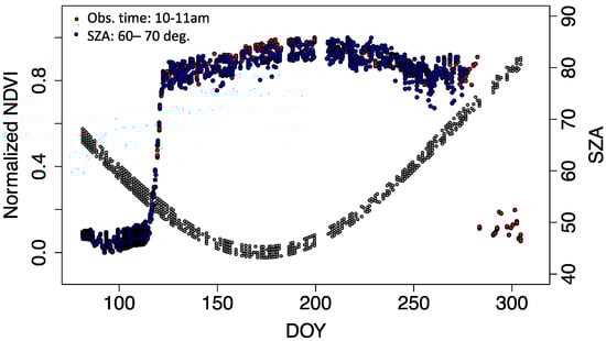
Figure 5.
Seasonal course of the normalized NDVI (=(NDVI − NDVImin)/(NDVImax − NDVImin)). Red circles are the measurements near the morning satellite overpass timings (10 to 11 am in AKST). Blue circles are the NDVI measurements when the solar zenith angle was between 60° to 70°. Grey circles are solar zenith angles corresponding to the morning satellite overpass timings (10 to 11 am in AKST).
3.3. NEE and NDVI-Based SOS and EOS Timings
The normalized NDVIsat time-series averaged each day reflected the overall trajectory of the seasonal change of NEE (Figure 6a). The NEE started decreasing at exactly the same point as the start of the NDVI green-up date (DOY 115). Then, normalized NDVIsat was 0.27 on the spring NEE zero crossing date (DOY 118) and was 0.83 on the autumn NEE zero crossing date (DOY 247). Outside of snow season (DOY 122 to 282), the amplitude of normalized NDVIsat accounted for 0.183 (18.3%) of the total NDVI seasonal amplitude. The autumn high plateau period (DOY 255 to DOY 282) was out of the photosynthetically active period. Both the NDVI increase from spring to summer and decrease from the summer to autumn were linearly correlated with NEE (Figure 6b). The slopes of the regression in autumn (=−8.50) were larger than that in spring (=−3.49), indicating that autumn NDVI was less sensitive to plant phenological activity.
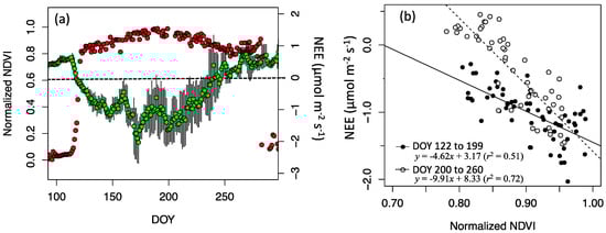
Figure 6.
(a) Seasonal changes in daily NEE (green circles) and mean normalized NDVI (red circles) between 10 am to 11 am. The five days moving window average was applied to the daily NEE data. Errorbars indicate the standard deviation of the moving window average. (b) Linear regressions between normalized NDVIsat and NEE in the spring-to-summer period (DOY 122 to 199) and the summer-to-autumn period (DOY 200 to 260).
4. Discussion
4.1. Influence of Solar Zenith Angle in NDVI Seasonality
We found that the slopes of the NDVI-SZA varied with phenological stages from positive (Stage A & B) to weak negative (stage B & C) (Figure 3 and Figure 4). In autumn, the NDVI-SZA slope stayed nearly constant (stage D). On the snowy understory conditions, canopy scale NDVIs in evergreen needleleaf forests are slightly higher than that of deciduous forests because of the existence of green colored needles [24]. The positive NDVI-SZA slopes in stage A and early stage B can be explained by two combined effects: the enhancement of the reflected signal from needles and the increase in the shadow area of black spruce trees. The weak negative NDVI-SZA slopes in the later stage B and stage C were primarily caused by the slight increase in the Red reflectance (Figure A2). Unlike the NDVI-SZA slope in stage A, the NDVI-SZA slopes in the later stage B and stage C potentially became positive or negative. Either positive or negative could depend on the forest structures and optical properties of tree elements (needles, trunk, and branch) vs understory plants.
Understanding how solar geometry affects the seasonal course of NDVI and spectral reflectance would help understanding how plant phenology affects the seasonal course of NDVI and spectral reflectance. From the comparisons between NDVI of the morning satellite over pass time (NDVIsat) and the standardized NDVI at 60–70° (NDVIsza), we found they had similar seasonal patterns as a whole (Figure 4). However, the timings of the annual peak were different. The earlier peak of NDVIsat was caused by the higher NDVI in the lower solar zenith angle in (Figure 3 left. stage C). The solar zenith angle at the satellite overpass time varied seasonally and latitudinally (Figure 4), therefore, the NDVI time-series must contain the effect of variable solar zenith angle. Earlier or later shifts of NDVI peaks could depend on the NDVI-SZA slope in the summer season and it eventually originated from the contrast of NDVI between canopy scale and understory. General features of the variable NDVI and spectral reflectance caused by sun geometries are taken into account in the inversion scheme of the ecosystem parameter estimations such as LAI and fraction of absorbed photosynthetically active radiation (e.g., [45,46]). However, the extremely sparse black spruce forest conditions in terms of their optical and structural characteristics is often off the global model representations. Our high-frequency spectral reflectance measurements, as well as forest optical and structure measurements, could contribute to the algorithm improvement of the ecosystem parameter retrievals in sparse boreal forests.
4.2. Canopy Scale and Understory Spectral Signatures
The separate measurements of canopy scale and understory spectral reflectance showed different seasonal and angular behaviors. Unlike the canopy scale NDVI, the understory NDVI were less affected by the vertical canopy structures. Therefore, the NDVI signals were nearly constant from stage A to C (Figure 3). The difference of angular dependencies of understory and canopy scale NDVI is an important phenomenon for remote sensing applications. For example, Yang et al. [32] developed a semi-empirical algorithm for retrieving understory NDVI from MODIS bi-directional reflectance distribution function (BRDF) data based on the assumption that the angular variations of understory NDVI were smaller than that of canopy scale NDVI. Results of this study (as shown in Figure 3 and Figure 4) practically verified this assumption using in situ measurements by indicating that the understory NDVI was less sensitive to variations of solar zenith angles than canopy scale NDVI. This partially guarantees the applicability of the method of Yang et al. [32] in this field.
4.3. Plant Phenology as Observed by In Situ Spectral Measurements
The continuous in situ measurements of spectral reflectance provide the ground truth of seasonal patterns in in situ NDVI. One of the important outcomes was the detection of the summer to autumn NDVI profile, which has rarely been observed from satellite observations because of frequent clouds and snows. Previous radiative transfer analysis implied the existence of an autumn high plateau [22] and explained that NDVI in the understory senescence period still keeps higher levels than the snowy surface and as the solar zenith angle becomes higher, the reflected signal from green evergreen needles becomes larger. We confirmed that the prediction by Kobayashi et al. [22] is correct. What matters is that nearly one month long high plateau was completely out of the plant photosynthetically active periods (Figure 6). The NDVI signal associated with the EOS timing (NEE zero crossing) falls at the beginning of the autumn high plateau. Previous studies proposed the satellite-based phenology algorithms to determine SOS and EOS ([47]). Because, in boreal evergreen needleleaf forests, seasonal NDVI profiles are not symmetric shapes about the mid-summer (DOY ~200), the application of the same phenology algorithms to both spring and autumn does not give the representative phenology. By calibrating the phenology data, Beck et al. [48] determined the autumn EOS threshold as normalized NDVI of 75% level. Also, this study obtained the autumn EOS threshold of the normalized NDVI of 83% (0.83) level. They were similar, but more importantly, the level of NDVI threshold in EOS depends on the understory NDVI and canopy openness and they are not necessarily to be a universal constant.
Outside the autumn plateau periods, the NDVI profile observed in this study was similar to that of satellite observations. However, the NDVI increase in spring and decrease in late autumn were more abrupt. The spring increase happened in 7 days (DOY 115 to 122) and the autumn decrease did so in 1 day (DOY 283). They are less than typical satellite compositing periods (eight to ten days), thus satellite-based temporal compositing data are prone to present smoother seasonal profiles. The comparison between seasonal NDVI profile and NEE shows the duration of the upper 20% of NDVI amplitude accounts for 95% of the photosynthetically active period (from DOY 122 to 247) (Figure 6). This means, without the snow effect, the actual NDVI changes in boreal evergreen forests are low. Thus, unlike temperate forests [49], NDVI becomes very sensitive in response to NEE. Particularly in the summer to autumn period, the NDVI sensitivity to NEE is twice as much as that of spring to summer (Figure 6).
4.4. Uncertainty
Although we carefully screened out and calibrated the highly uncertain measurements, potential uncertainty of the spectral reflectance might be contaminated in particular to the measurements at the top of the tower. To correct the tower reflection effect, we compared the measurements with the narrower spectroradiometer measurements (FOV = 25°). The comparisons showed no significant bias trends regarding the local time and DOY, and thus we applied the constant bias subtraction to Red and near infrared reflectances throughout the year. However, to quantify more reliable NDVIs including their absolute values, it is necessary to remove the effect of artificial tower structure by shielding the scaffold tower by completely black materials. In addition, differences in the footprints from tower-mounted and understory spectroradiometer might also affect the representativeness of the forest site. We installed the spectroradiometer on a typical understory surface around the site (mixture of shrubs and sedges on the moss and lichen surfaces), thus spectral reflectance obtained on the understory measurements were thought to be comparable, but the evaluation of the representativeness by measuring the spatial understory reflectances warrants the validity of the assumption.
The understory measurements were also the mixture of shadow and illuminated surfaces. The shadows were cast by the neighboring trees and shrubs, and the mutual shadows of understory species. A typical example is shown in Figure A1 in Appendix C. The understory image in DOY 122 shows the horizontal shadow zone in the bottom edge of the white lichen community. When the shadow and illuminated surface are mixed in the sensor’s field of view, the reflectance information are weighted by the illuminated area. In this study, we could not separate the impact of shadows. Further observations with multiple spectoradiometer deployments are necessary to evaluate the spatially representative seasonality in understory reflectance.
Our in situ measurements are directional-hemispherical reflectance or bi-hemispherical reflectance obtained near the top of the canopy and understory level. These are not the exact same quantities as the satellite-based bidirectional reflectance observations. Thus, those in situ measurements may not present the same reflectance anisotropy and spectral characteristics. The use of in situ measurements for the comparison with satellite observations will need a careful attention due to the inherent uncertainty owing to the observation principle.
5. Conclusions
We present the in situ spectral measurements in an open black spruce forest. In our analysis, the followings were found. (1) Canopy scale NDVI varied with solar zenith angle, and the slope of NDVI-SZA also varied seasonally from positive in fully snow-covered understory to weak positive in the summer. Understory NDVI was less sensitive than canopy scale NDVI; (2) The NDVI maximum peak timing in the summer was affected by the solar zenith angle; (3) The autumn high NDVI plateau was clearly detected. This autumn plateau was completely out of the photosynthetically active periods. The EOS timings evaluated from the NEE zero crossing date was corresponded to the start of the autumn high plateau. In this way, our spectral measurements can be served as baseline information for the development and validation of satellite-based phenology algorithms in the northern high latitudes.
Author Contributions
Conceptualization, H.K. W.Y.; Methodology, H.K., S.N., Y.K., H.N., R.S.; Formal Analysis, H.K., K.I., H.I., Writing-Original Draft Preparation, H.K.; Writing-Review & Editing, H.K., W.Y., S.N., Y.K., H.N., H.I., K.I.
Funding
This study was supported by JAXA GCOM-C RA #111, JSPS Grant-in-Aid for Scientific Research (B) # 16H02948, and JAMSTEC and IARC/UAF collaboration study (JICS) and Arctic Challenge for Sustainability Project (ArCS).
Acknowledgments
We thank Bob Busey and Go Iwahana in IARC/UAF for the site maintenance and data management.
Conflicts of Interest
The authors declare no conflict of interest.
Appendix A. Spectral Reflectance Measurements
Two visible and near infrared spectroradiometer systems, MS-700 (Eko Instruments Co., Ltd.) and rotating platforms (Hayasaka Rikoh Co., Ltd.) [43] were installed at the study site in March 2015 for the canopy scale and understory reflectance measurements (Figure 1). The study site around the spectroradiometers constitutes the typical tree stand conditions on the flat surface. To measure the canopy scale reflectance, one MS-700 sensor was put on the top of the scaffold tower. On the top of the tower (height = 17 m), the MS-700 sensor was mounted on a rotating platform attached in the forefront of a 1.0 m-long slide rail and was set to magnetic north (Figure 1a). To measure the understory reflectance, the other MS-700 was installed at 1.5 m height with a tripod situated at approximately 20 m northwest of the tower (Figure 1b). This understory MS-700 system was also laid on a rotating platform in the forefront of a slide rail. The rotating platforms moved up and down (zenith angle: 0° to 180°) to measure the incoming sky radiation, as well as reflected radiation from the surface. The field of view of the MS-700 systems is 180° (hemisphere). The wavelength range of MS-700 was 350 to 1050 nm with a spectral resolution of 10 nm (full width half maximum). The alignment error of the wavelength was less than 0.3 nm. The exposure time was automatically optimized in each measurement within a range of 0.01 s–5 s. The incoming radiation was received by a cosine collector on the detector with a glass filter dome. Thus, the measured quantities by the MS-700 were hemispherical irradiance.
Daily spectral reflectance measurements were scheduled from 7 am to 7 pm on Alaska Standard Time (AKST) with an interval of two minutes. Generally, the MS-700 systems were faced upward and measured the incoming sky radiation. The rotating platform turns over every 10 min for the surface reflected radiation measurements. Therefore, the sequences of the hourly sky radiation measurements were recorded at 02 min, 04 min, 06 min, 08 min, 12 min, 14 min, and so on. The measurements at 00 min and 10 min were skipped because of the surface measurements. Likewise, the sequences of the hourly surface radiation measurements were 00 min, 10 min, 20 min, 30 min, 40 min, and 50 min. The spectral reflectance was quantified from every 10 min’ surface measurements and an average of two nearest neighbor sky radiation measurements. For example, spectral reflectance at 10:20 was computed from sky measurements at 10:18 and 10:22 and the surface measurement at 10:20.
The hemispherical reflectance measurements at the top of the tower could be partially affected by the reflection from scaffold structure. To calibrate the reflectance from the MS-700 system, another field spectroradiometer system, which had a narrower field of view, was installed next to the MS-700 spectroradiometer system in 2017. This system contained a spectroradiometer (HR4000, Ocean Optics, Inc., FWHM = 0.2 nm, field of view = 25°) and two 30 m long optical fibers. A cosine collector was attached to the optical fiber that was directed at the sky. The other optical fiber was directed to the surface with the view zenith angle of 45° and the magnetic north direction. The time lags of the spectral radiation measurements from the sky and the surface were less than 3 s. Bi-directional spectral reflectance factors were computed from the sky, the surface measurements, and the sensor’s dark current.
Appendix B. Quality Control, Reflectance Calibration and Data Processing
Because of the four-minute time lag between two sky measurements taken before and after the surface spectral measurements, the computed reflectances from the MS-700 systems were affected by the short-term variations in solar radiation. To remove the erroneous reflectance data, we evaluated the level of differences between sky measurements ():
where Isky1 and Isky2 are the first and second sky measurements. We removed the reflectance data with > 5%. Additional screening was applied for the reflectance data measured at the tower top. The data on the tower around local noon time (12:00 to 14:00) contained the forward reflection from the scaffold structure. We removed the data measured between 12:00–14:00 from our analysis. Finally, the fraction and number of valid data in 2017 were N = 5547 out of 17,370 (33.9%) for the tower measurements and N = 6717 out of 17,370 (41.0%) for the understory measurements. The spectral reflectances in Red and NIR were computed as close as the wavelength range of Terra-MODIS band 1 (620–670 nm) and band 2 (841–876 nm), respectively. They were derived by the spectral averages in 621.3–671.3 nm (Red) and 840.2–876.3 nm (NIR).
Although we removed the measurements that were highly affected by the tower reflection, other measurements contained a residual offset by the tower reflection. To re-calibrate the reflectance data, we compared the alternate reflectance data measured by the narrower field of view sensor (HR4000). We extracted the HR4000 spectral reflectance in Red and NIR that were measured at exactly the same time for MS-700 measurements. By comparing Red and NIR reflectance throughout the growing season, we quantified the biases in Red and NIR measurements (bias = −0.0219 in Red, bias = 0.054 in NIR). The Red and NIR reflectance products for the tower measurements were computed by subtracting those biases.
Appendix C Time-Lapse Camera Images
The states of canopy and understory were observed by the time-lapse cameras. The details of the observation conditions were described in 2.4. Figure A1 are time-sequential images in the typical tipping points in NDVI shown in Figure 2. Those images clearly show the snow coverage, black spruce tree stands, and greenness of the understory plants.

Figure A1.
Time-lapse camera images obtained at the top of the tower and understory.
Appendix D Solar Zenith Angle Dependency of Red and NIR Reflectances
In addition to NDVI shown in Figure 3, spectral reflectance in Red and near infrared (NIR) also varies with the solar zenith angles. Figure A2 and Figure A3 show the solar zenith angle dependency of Red and NIR reflectances.

Figure A2.
Solar zenith angle dependency of Red in five phenological stages. The definition of phenological stages are shown in Figure 2. Left: canopy Red (measured at the top of the tower). Right: understory measurements. Colors on the plotted circles denote the DOY of the measurements.

Figure A3.
Solar zenith angle dependency of NIR reflectance in five phenological stages. The definition of phenological stages are shown in Figure 2. Left: canopy scale NIR reflectance (measured at the top of the tower). Right: understory measurements. Colors on the plotted circles denote the day of the year (DOY) of the measurements.
References
- IPCC. Climate Change 2013: The Physical Science Basis. Contribution of Working Group I to the Fifth Assessment Report of the Intergovernmental Panel on Climate Change; Cambridge University Press: Cambridge, UK; New York, NY, USA, 2014. [Google Scholar]
- Hinzman, L.D.; Bettez, N.D.; Bolton, W.R.; Chapin, F.S.; Dyurgerov, M.B.; Fastie, C.L.; Griffith, B.; Hollister, R.D.; Hope, A.; Huntington, H.P.; et al. Evidence and implications of recent climate change in Northern Alaska and other Arctic regions. Clim. Chang. 2005, 72, 251–298. [Google Scholar] [CrossRef]
- Bekryaev, R.V.; Polyakov, I.V.; Alexeev, V.A. Role of polar amplification in long-term surface air temperature variations and modern arctic warming. J. Clim. 2010, 23, 3888–3906. [Google Scholar] [CrossRef]
- AMAP. Snow, Water, Ice and Permafrost. Summary for Policy-Makers; Arctic Monitoring and Assessment Programme (AMAP): Oslo, Norway, 2017. [Google Scholar]
- Euskirchen, E.S.; McGuire, A.D.; Chapin, F.S.; Rupp, T.S. The changing effects of Alaska’s boreal forests on the climate system. Can. J. For. Res. 2010, 40, 1336–1346. [Google Scholar] [CrossRef]
- Chapin, F.S., III; McFarland, J.; McGuire, A.D.; Euskirchen, E.S.; Ruess, R.W.; Kielland, K. The changing global carbon cycle: Linking plant–soil carbon dynamics to global consequences. J. Ecol. 2009, 97, 840–850. [Google Scholar]
- Barichivich, J.; Briffa, K.R.; Myneni, R.B.; Osborn, T.J.; Melvin, T.M.; Ciais, P.; Piao, S.; Tucker, C. Large-scale variations in the vegetation growing season and annual cycle of atmospheric CO2 at high northern latitudes from 1950 to 2011. Glob. Chang. Biol. 2013, 19, 3167–3183. [Google Scholar] [CrossRef] [PubMed]
- Forkel, M.; Carvalhais, N.; Rödenbeck, C.; Keeling, R.; Heimann, M.; Thonicke, K.; Zaehle, S.; Reichstein, M. Enhanced seasonal CO2 exchange caused by amplified plant productivity in northern ecosystems. Science 2016, 351, 696–699. [Google Scholar] [CrossRef] [PubMed]
- Sato, H.; Kobayashi, H.; Iwahana, G.; Ohta, T. Endurance of larch forest ecosystems in eastern Siberia under warming trends. Ecol. Evol. 2016, 6, 5690–5704. [Google Scholar] [CrossRef] [PubMed]
- Wang, L.; Fensholt, R. Temporal changes in coupled vegetation phenology and productivity are biome-specific in the Northern Hemisphere. Remote Sens. 2017, 9, 1–18. [Google Scholar]
- Graven, H.D.; Keeling, R.F.; Piper, S.C.; Patra, P.K.; Stephens, B.B.; Wofsy, S.C.; Welp, L.R.; Sweeney, C.; Tans, P.P.; Kelley, J.J.; et al. Enhanced seasonal exchange of CO2 by northern ecosystems since 1960. Science 2013, 341, 1085–1089. [Google Scholar] [CrossRef] [PubMed]
- Myneni, R.B.; Keeling, C.D.; Tucker, C.J.; Asrar, G.; Nemani, R.R. Increased plant growth in the northern high latitudes from 1981 to 1991. Nature 1997, 386, 698–702. [Google Scholar] [CrossRef]
- Delbart, N.; Picard, G.; Toan, T.L.; Kergoat, L.; Quegan, S.; Woodward, I.; Dye, D.; Fedotova, V. Spring phenology in boreal Eurasia over a nearly century time scale. Glob. Chang. Biol. 2008, 14, 603–614. [Google Scholar] [CrossRef]
- Garonna, I.; De Jong, R.; De Wit, A.J.W.; Mucher, C.A.; Schmid, B.; Schaepman, M.E. Strong contribution of autumn phenology to changes in satellite-derived growing season length estimates across Europe (1982–2011). Glob. Chang. Biol. 2014, 20, 3457–3470. [Google Scholar] [CrossRef] [PubMed]
- Buermann, W.; Parida, B.; Jung, M.; MacDonald, G.M.; Tucker, C.J.; Reichstein, M. Recent shift in Eurasian boreal forest greening response may be associated with warmer and drier summers. Geophys. Res. Lett. 2014, 41, 1995–2002. [Google Scholar] [CrossRef]
- Piao, S.; Wang, X.; Ciais, P.; Zhu, B.; Wang, T.; Liu, J. Changes in satellite-derived vegetation growth trend in temperate and boreal Eurasia from 1982 to 2006. Glob. Chang. Biol. 2011, 17, 3228–3239. [Google Scholar] [CrossRef]
- Xu, L.; Myneni, R.B.; Chapin, F.S., III; Callaghan, T.V.; Pinzon, J.E.; Tucker, C.J.; Zhu, Z.; Bi, J.; Ciais, P.; Tømmervik, H.; et al. Temperature and vegetation seasonality diminishment over northern lands. Nat. Clim. Chang. 2013, 3, 581–586. [Google Scholar] [CrossRef]
- White, M.A.; Thornton, P.E.; Running, S.W. A continental phenology model for monitoring vegetation responses to interannual climatic variability. Glob. Biogeochem. Cycles 1997, 11, 217–234. [Google Scholar] [CrossRef]
- Zhang, X.; Friedl, M.A.; Schaaf, C.B.; Strahler, A.H.; Hodges, J.C.F.; Gao, F.; Reed, B.C.; Huete, A. Monitoring vegetation phenology using MODIS. Remote Sens. Environ. 2003, 84, 471–475. [Google Scholar] [CrossRef]
- Delbart, N.; Kergoat, L.; Toan, T.L.; Lhermitte, J.; Picard, G. Determination of phenological dates in boreal regions using normalized difference water index. Remote Sens. Environ. 2005, 97, 26–38. [Google Scholar] [CrossRef]
- Dye, D.G.; Tucker, C.J. Seasonality and trends of snow-cover, vegetation index, and temperature in northern Eurasia. Geophys. Res. Lett. 2003, 30. [Google Scholar] [CrossRef]
- Kobayashi, H.; Yunus, A.P.; Nagai, S.; Sugiura, K.; Kim, Y.; Dam, B.V.; Nagano, H.; Zona, D.; Harazono, Y.; Bret-Harte, M.S.; et al. Latitudinal gradient of spruce forest understory and tundra phenology in, Alaska as observed from satellite and ground-based data. Remote Sens. Environ. 2016, 177, 160–170. [Google Scholar] [CrossRef]
- Kobayashi, H.; Suzuki, R.; Kobayashi, S. Reflectance seasonality and its relation to the canopy leaf area index in an eastern Siberian larch forest: Multi-satellite data and radiative transfer analyses. Remote Sens. Environ. 2007, 106, 238–252. [Google Scholar] [CrossRef]
- Suzuki, R.; Kobayashi, H.; Delbart, N.; Asanuma, J.; Hiyama, T. NDVI responses to the forest canopy and floor from spring to summer observed by airborne spectrometer in eastern Siberia. Remote Sens. Environ. 2011, 115, 3615–3624. [Google Scholar] [CrossRef]
- Zhu, W.; Tian, H.; Xu, X.; Pan, Y.; Chen, G.; Lin, W. Extension of the growing season due to delayed autumn over mid and high latitudes in North America during 1982–2006. Glob. Ecol. Biogeogr. 2012, 21, 260–271. [Google Scholar] [CrossRef]
- Delpierre, N.; Dufrêne, E.; Soudani, K.; Ulrich, E.; Cecchini, S.; Boé, J.; François, C. Modelling interannual and spatial variability of leaf senescence for three deciduous tree species in France. Agric. For. Meteorol. 2009, 149, 938–948. [Google Scholar] [CrossRef]
- Richardson, A.D.; Keenan, T.F.; Migliavacca, M.; Ryu, Y.; Sonnentag, O.; Toomey, M. Climate change, phenology, and phenological control of vegetation feedbacks to the climate system. Agric. For. Meteorol. 2013, 169, 156–173. [Google Scholar] [CrossRef]
- Jönsson, M.; Eklundh, L.; Hellström, M.; Bärring, L.; Jönsson, P. Annual changes in MODIS vegetation indices of Swedish coniferous forests in relation to snow dynamics and tree phenology. Remote Sens. Environ. 2010, 114, 2719–2730. [Google Scholar] [CrossRef]
- Eriksson, H.M.; Eklundh, L.; Kuusk, A.; Nilson, T. Impact of understory vegetation on forest canopy reflectance and remotely sensed LAI estimates. Remote Sens. Environ. 2006, 103, 408–418. [Google Scholar] [CrossRef]
- Lu, H.; Raupach, M.R.; McVicar, T.R.; Barrett, D.J. Decomposition of vegetation cover into woody and herbaceous components using AVHRR NDVI time series. Remote Sens. Environ. 2003, 86, 1–18. [Google Scholar] [CrossRef]
- Pisek, J.; Chen, J.M.; Kobayashi, H.; Rautiainen, M.; Schaepman, M.E.; Karnieli, A.; Sprinstin, M.; Ryu, Y.; Nikopensius, M.; Raabe, K. Retrieval of seasonal dynamics of forest understory reflectance from semiarid to boreal forests using MODIS BRDF data. J. Geophys. Res. Biogeosci. 2016, 121, 855–863. [Google Scholar] [CrossRef]
- Yang, W.; Kobayashi, H.; Suzuki, R.; Nasahara, K.N. A simple method for retrieving understory NDVI in sparse needleleaf forests in Alaska using MODIS BRDF data. Remote Sens. 2014, 6, 11936–11955. [Google Scholar] [CrossRef]
- Rautiainen, M.; Mõttus, M.; Heiskanen, J.; Akujärvi, A.; Majasalmi, T.; Stenberg, P. Seasonal reflectance dynamics of common understory types in a northern European boreal forest. Remote Sens. Environ. 2011, 115, 3020–3028. [Google Scholar] [CrossRef]
- Rautiainen, M.; Heiskanen, J. Seasonal contribution of understory vegetation to the reflectance of a boreal landscape at different spatial scales. Geosci. Remote Sens. Lett. 2013, 10, 923–927. [Google Scholar] [CrossRef]
- Miller, J.R.; White, H.P.; Chen, J.M.; Peddle, D.R.; McDermid, G.; Fournier, R.A.; Shepherd, P.; Rubinstein, I.; Freemantie, J.; Soffer, R.; et al. Seasonal change in understory reflectance of boreal forests and influence on canopy vegetation indices. J. Geophys. Res. 1997, 102, 29475–29482. [Google Scholar] [CrossRef]
- Nakai, T.; Kim, Y.; Busey, R.C.; Suzuki, R.; Nagai, S.; Kobayashi, H.; Park, H.; Sugiura, K.; Ito, A. Characteristics of evapotranspiration from a permafrost black spruce forest in interior Alaska. Polar Sci. 2013, 7, 136–148. [Google Scholar] [CrossRef]
- Ikawa, H.; Nakai, T.; Busey, R.C.; Kim, Y.; Kobayashi, H.; Nagai, S.; Ueyama, M.; Saito, K.; Nagano, H.; Suzuki, R.; et al. Understory CO2, sensible heat, and latent heat fluxes in a black spruce forest in interior Alaska. Agric. For. Meteorol. 2015, 214–215, 80–90. [Google Scholar] [CrossRef]
- Sugiura, K.; Suzuki, R.; Nakai, T.; Busey, B.; Hinzman, L.; Park, H.; Kim, Y.; Nagai, S.; Saito, K.; Cherry, J.; et al. Supersite as a common platform for multi-observations in Alaska for a collaborative framework between JAMSTEC and IARC. JAMSTEC Rep. Res. Dev. 2011, 12, 61–69. [Google Scholar] [CrossRef]
- Kobayashi, H.; Suzuki, R.; Nagai, S.; Nakai, T.; Kim, Y. Spatial scale and landscape heterogeneity effects on FAPAR in an open-canopy black spruce forest in interior Alaska. IEEE Geosci. Remote Sens. Lett. 2014, 11, 564–568. [Google Scholar] [CrossRef]
- Suzuki, R.; Kim, Y.; Ishii, R. Sensitivity of the backscatter intensity of ALOS/PALSAR to the above-ground biomass and other biophysical parameters of boreal forest in Alaska. Polar Sci. 2013, 7, 100–112. [Google Scholar] [CrossRef]
- Sugiura, K.; Nagai, S.; Nakai, T.; Suzuki, R. Application of time-lapse digital imagery for ground-truth verification of satellite indices in the boreal forests of Alaska. Polar Sci. 2013, 7, 149–161. [Google Scholar] [CrossRef]
- Nagai, S.; Nakai, T.; Saitoh, T.M.; Busey, R.C.; Kobayashi, H.; Suzuki, R.; Muraoka, H.; Kim, Y. Seasonal changes in camera-based indices from an open canopy black spruce forest in Alaska, and comparison with indices from a closed canopy evergreen coniferous forest in Japan. Polar Sci. 2013, 7, 125–135. [Google Scholar] [CrossRef]
- Nasahara, K.N.; Nagai, S. Development of an in situ observation network for terrestrial ecological remote sensing: The Phenological Eyes Network (PEN). Ecol. Res. 2015, 30, 211–223. [Google Scholar] [CrossRef]
- Nagai, S.; Akitsu, T.; Saitoh, T.M.; Busey, R.C.; Fukuzawa, K.; Honda, Y.; Ichie, T.; Ide, R.; Ikawa, H.; Iwasaki, A.; et al. 8 million phenological and sky images from 29 ecosystems from the Arctic to the tropics: The Phenological Eyes Network. Ecol. Res. 2018. [Google Scholar] [CrossRef]
- Myneni, R.B.; Hoffman, S.; Knyazikhin, Y.; Privette, J.L.; Glassy, J.; Tian, Y.; Wang, Y.; Song, X.; Zhang, Y.; Smith, G.R.; et al. Global products of vegetation leaf area and fraction absorbed PAR from year one of MODIS data. Remote Sens. Environ. 2002, 83, 214–231. [Google Scholar] [CrossRef]
- Knyazikhin, Y.; Martonchik, J.V.; Myneni, R.B.; Diner, D.J.; Running, S.W. Synergistic algorithm for estimating vegetation canopy leaf area index and fraction of absorbed photosynthetically active radiation from MODIS and MISR data. J. Geophys. Res. 1998, 103, 32257–32275. [Google Scholar] [CrossRef]
- White, M.A.; de Beurs, K.M.; Didan, K.; Inouye, D.W.; Richardson, A.D.; Jensen, O.P.; O’Keefe, J.; Zhang, G.; Nemani, R.R.; Leeuwen, W.J.D.V.; et al. Intercomparison, interpretation, and assessment of spring phenology in North America estimated from remote sensing for 1982–2006. Glob. Chang. Biol. 2009, 15, 2335–2359. [Google Scholar] [CrossRef]
- Beck, P.S.A.; Jönsson, P.; Høgda, K.A.; Karlsen, S.R.; Eklundh, L.; Skidmore, A.K. A ground-validated NDVI dataset for monitoring vegetation dynamics and mapping phenology in Fennoscandia and the Kola peninsula. Int. J. Remote Sens. 2007, 28, 4311–4330. [Google Scholar] [CrossRef]
- Muraoka, H.; Noda, H.M.; Nagai, S.; Motohka, T.; Saitoh, T.M.; Nasahara, K.N.; Saigusa, N. Spectral vegetation indices as the indicator of canopy photosynthetic productivity in a deciduous broadleaf forest. J. Plant Ecol. 2013, 6, 393–407. [Google Scholar] [CrossRef]
© 2018 by the authors. Licensee MDPI, Basel, Switzerland. This article is an open access article distributed under the terms and conditions of the Creative Commons Attribution (CC BY) license (http://creativecommons.org/licenses/by/4.0/).