Abstract
This study evaluated whether wavelet functions (Bior1.3, Bior2.4, Db4, Db8, Haar, Sym4, and Sym8) and decomposition levels (Levels 3–8) can estimate soil properties. The analysis is based on the discrete wavelet transform with partial least-squares (DWT–PLS) method, incorporated into a visible and near-infrared reflectance analysis. The improved DWT–PLS method (called DWT–Stepwise-PLS) enhances the accuracy of the quantitative analysis model with DWT–PLS. The cation exchange capacity (CEC) was best estimated by the DWT–PLS model using the Haar wavelet function. This model yielded the highest coefficient of determination (Rv2 = 0.787, p < 0.001), with the highest relative percentage deviation (RPD = 2.047) and lowest root mean square error (RMSE = 4.16) for the validation data set of the CEC. The RPD of the SOM predictions by DWT–PLS using the Bior1.3 wavelet function was maximized at 1.441 (Rv2 = 0.642, RMSE = 5.96), highlighting the poor overall predictive ability of soil organic matter (SOM) by DWT–PLS. Furthermore, the best performing decomposition levels of the wavelet function were distributed in the fifth, sixth, and seventh levels. For various wavelet functions and decomposition levels, the DWT–Stepwise-PLS method more accurately predicted the quantified soil properties than the DWT–PLS model. DWT–Stepwise-PLS using the Haar wavelet function remained the best choice for quantifying the CEC (Rv2 = 0.92, p < 0.001, RMSE = 4.91, and RPD = 3.57), but the SOM was better predicted by DWT–Stepwise-PLS using the Bior2.4 wavelet function (Rv2 = 0.8, RMSE = 5.34, and RPD = 2.24) instead of the Bior1.3 wavelet function. However, the performance of the DWT–Stepwise-PLS method tended to degrade at high and low decomposition levels of the DWT. These degradations were attributed to a lack of sufficient information and noise, respectively.
1. Introduction
Soil quality mainly depends on the chemical and physical properties of the soil, which are estimated by the cumulative effects of natural factors involved in its formation, including climate, topography, parent material, biological activity, and time [1]. The development of precision agriculture requires a quantitative analysis technology that can accurately and quickly elucidate the physicochemical properties of soils over a large area. Routine soil testing is recognized as basic techniques for estimating soil properties [2]; however, the traditional soil testing and granulometric analyses are relatively slow and expensive, because a large number of soil samples is needed for mapping the spatial variation in the managed field [3].
The visible and near infrared reflectance analysis (Vis-NIRA) technique has emerged as a possible enhancer or replacer of traditional soil testing methods. Using the Vis-NIRA technique, many researchers have related soil properties to spectroscopic soil reflectance data [4,5,6,7,8,9,10,11]. However, because the extremely large volume of hyper-spectral data and visible and near-infrared hyper-spectra are difficult to interpret directly, since they contain overlapping weak overtones and combinations of fundamental vibrational bands, identifying the critical spectral features that estimate the soil properties is a difficult task.
Besides containing many redundancies, soil reflectance hyper-spectral data are affected by the soil surface roughness, soil moisture, various environmental noises, and various other factors [12]. Therefore, to provide a good dataset for soil reflectance spectroscopy, the noise should be removed as far as possible while preserving the spectral details. The discrete wavelet transform (DWT) is a wavelet transform technique that extracts the features of hyper-spectral data, and has been popularly applied to spectroscopic analysis [7,13,14,15,16,17]. The DWT is an integral transformation, but can be decomposed into a set of coefficients. In this way, the DWT can combine a set of mathematical building blocks (basic functions) and reorganize the original data. The DWT transforms the eigenvalues obtained by detailed and approximate signals, generating the coefficients as raw data containing the vast majority of the original data characteristics, which is an important way of reducing the data dimensions [7,15]. The DWT is considered as an excellent method for predicting multiple soil properties. However, although the scale of wavelet analysis has been discussed [14], the impact of multiple wavelet functions on the prediction of soil properties has not been well studied. The widely varying properties of the different wavelet functions will certainly affect the predicted soil properties. Therefore, this paper will explore how different wavelet functions affect the prediction model of soil properties.
Predictive models are generally calibrated using the measured spectral datasets of soils with known properties, and such datasets are assembled into spectral libraries [18]. The most popular spectroscopic analysis methods are multiple linear regression (MLR), principal coefficients regression (PCR), partial least-squares regression (PLS), and artificial neural networks (ANN) [6,19,20,21]. Partial least-squares regression and multiple linear stepwise regression are considered the most appropriate regression methods for spectral calibration and prediction of soil properties [22,23,24]. PLS has the same overall framework as principal component regression, and includes multiple regression and canonical correlation analyses [25]. As such, it can predict the number of suitable variables and eliminate noise interference, retaining the useful data for traditional linear regression. Moreover, PLS can extract the main determinant variables from soil reflectance spectroscopy data, reducing the spectral dimension and enhancing the robustness of the established model. However, the PLS method is inapplicable to data containing much useless information, because some of the independent variables can be misinterpreted as explanatory powers and incorporated into the regression equation, reducing the model accuracy [26]. Hyper-spectral data, which include a large volume of redundant information and noise-distorted spectral shapes, fall into this category. The spectral noise is introduced by sensor limitations and particle-size differences [27]. Hence, improving the PLS method for statistical analysis of spectral data has become a main research focus [28,29,30]. Multivariate stepwise linear regression (MSLR) finds and selects the variables exerting the most significant influences on the dependent variables and outperforms ordinary meta-regression; however, this method cannot remove the multi-collinearity between independent variables. In contrast, stepwise multiple regression combined with the partial least-squares method can preliminarily deduct the information unrelated to the response vector by an algebraic algorithm.
The main objectives of this study were as follows: (a) to characterize the representativeness of different wavelet functions and different decomposition scales in the prediction model, and (b) to understand appropriateness of the improved regression analysis (Stepwise-PLS) in improving the prediction accuracy of soil properties.
2. Materials and Methods
2.1. Soil Sample Preparation and Laboratory Analysis
For this study, 193 soil samples of Burozem and Cinnamon soil were collected from the Experimental Station of Qingdao Agricultural University (Shandong Province, China) in 2014. The main parent materials of Cinnamon soil consist of loess and lime, and its mineral composition is primarily hydromica, montmorillonite, and kaolinite. The main parent materials of Burozem soil are non-calcareous eluvial slope deposits and earthy deposits, and its mineral composition is primarily hydromica, kaolinite, and vermiculite. For one certain soil type, the soil samples have similar parent materials, mineral composition, and texture. The collected soil samples were air-dried for 72 h and then passed through a 4.75-mm aperture square-hole sieve to remove the coarse matter and organic debris. The physical and chemical properties of the soil were measured as described by I.S.S.C.A.S. (1978) [31]. Briefly, the soil organic matter (SOM) was estimated by K2Cr2O7 oxidation at 180 °C, and the cation exchange capacity (CEC) was estimated by displacing the exchangeable cations on the soil particle surfaces with NH4+. Each soil sample was measured in duplicate, and the main soil properties are summarized in Table 1.

Table 1.
Statistical description of soil properties in soil samples.
The hyper-spectral reflectance data were obtained from 350 to 2500 nm by an Analytical Spectral Device spectroradiometer with a spectral resolution of 1.4 nm. The collected soil samples were measured in a dark room in the laboratory. The field-of-view was 8°, and the illumination was provided by a 1000-W halogen lamp fixed 100 cm directly above the soil plane. To eliminate the effects of soil moisture as much as possible, the soil samples were naturally air dried before the hyper-spectral measurements. The soil samples were placed inside a circular black capsule with a diameter of 10 cm and depth of 1 cm, and were leveled to a smooth surface with the edge of a spatula. In the present laboratory experiments, the reflectance between each reflectance measurement was standardized using a white Spectralon reference panel [32]. The visible and near infrared reflectance spectra of the soil samples were converted to spectral reflectance by dividing them by the Spectralon reference panel. These first derivative transformations are known to minimize the sample variations caused by changes in the grinding and optical settings [21]. To eliminate the noise in the first derivative spectra, we applied Savitzky–Golay smoothing [33] to the original reflectance spectra curve. In addition, like most of the hyper-spectral prediction models of soil properties, this study takes the first derivative of the spectral reflectance as an independent variable. Prior to the data analysis, six soil samples yielded negative hyper-spectral data after the hyper-spectral measurements of all soil samples and were discarded from our analysis.
We classified the original soil samples prior to data analysis. Combined with some previous studies, there is a definite masking effect between soil properties. For example, Rossel’s studies [34] have confirmed that the masking of other constituents by organic matter in hyper-spectral reflectance is weakened by soil organic matter contents below 10 g/kg. Therefore, the classification of all soil samples is an essential preliminary work, in order to avoid the masking effect between soil properties. The soil samples were selected on the condition that the soil properties to be predicted varied significantly (with greater coefficients of variance (CV) values), whereas other properties changed slightly (with lower CV values). In this study, we grouped the soil samples with soil organic matter contents below 10 g/kg into the A group, which was used as the dataset for estimating CEC. On the other hand, the soil samples with CEC values below 20 cmol/g were selected into the B group, which was used as a data set for estimating SOM.
The soil samples were randomly selected from groups A and B at a 7:3 ratio to get calibration and validation data sets, respectively. The A group dataset (69 soil samples) was split into 49 randomly selected samples for calibration, and the remaining 20 soil samples were reserved for validation. Similarly, the B group dataset (114 soil samples) was split into 90 randomly selected samples for calibration, and 34 samples for validation. The soil properties in the soil samples are statistically described in Table 2.
Table 2.
Statistical description of soil properties in soil samples for groups A and B.
2.2. Discrete Wavelet Transform (DWT)
Wavelet analysis theory has been extensively reported in previous literature, so it is only briefly introduced here. DWT is ideally suited to spectral feature extraction, most fundamentally because it performs a multi-scale analysis of the signal [35]. DWT can be mathematically expressed as a finite length sequence and a discrete wavelet basis of the inner product, where each inner product factor is a discrete wavelet transform [13]. The DWT coefficients are expressed as follows:
where is the value of DWT coefficient; is a sequence of length n. The discrete wavelet basis is given by
where and correspond to the discrete wavelet scale and the translation parameters, respectively, and the superscript * denotes the complex conjugate. For a binary wavelet, = 2. To classify the detailed information into approximate scale categories, the hyper-spectral signal is projected onto a wavelet function. This approach is superior to other analytical methods. Unlike the Fourier transform, the scale transformation of a discrete wavelet transform is carried out on wavelets with non-unique and irregular fundamental waves, largely different waveforms of the fundamental waves, and largely different support lengths and regularity. The signal processing of different wavelet signals in the same signal often yields large differences among the results, which inevitably affects the final processing results. Therefore, the wavelet functions must be appropriately chosen for hyper-spectral pre-processing. The basic properties of the different wavelet functions available for DWT are given in Table 3.
Table 3.
Description of common wavelet function properties.
Based on some previous studies [7,15], we selected seven wavelet functions (Haar, Bior1.3, Bior2.4, Db4, Db8, Sym4, and Sym8), and explored their effects on the accuracy of the predicted model. Here, the DWT was performed with the Wavelet toolbox in MATLAB Release 12b (Matrix Laboratory, Math-Works, Natick, MA, USA).
2.3. Stepwise-Partial Regression Analysis
To eliminate the redundancy and noise in the hyper-spectral data, this study improves the partial least-squares fitting. The error terms in the partial least-squares regression model are not normally distributed, and their exact distribution is particularly difficult to discern. Therefore, the parameter significances, which determine the choice of variables, cannot be tested by evaluating the parameter statistics. Here we improve the partial least-squares model by proposing a variable selection method in MSLR, based on the fitting error. We refer to this method as Stepwise-PLS. This article briefly introduces the idea of improvement showed in Figure 1.
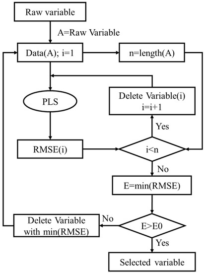
Figure 1.
Flowchart of Stepwise-PLS (partial least-squares regression).
In this improved algorithm, all of the original variables are used in the PLS model fitting, and the root-mean-square deviation (RMSE) is calculated as
where and are the actual and forecasted values, respectively.
The RMSE calculated by Equation (3) is set to E0. Next, one of the original variables are removed each time, until all variables have passed through, and the remaining variables are reinserted into the PLS model. The RMSE is calculated in each instance, and is set to E. The minimum value of RMSE is computed (E = min (RMSE)) and compared with E0. If E < E0, the variable corresponding to the minimum error is removed, presuming that its removal will improve the model precision. Conversely, if E > E0, then all of the unfavorable variables are rejected, and all remaining variables are deemed suitable for the PLS model. These series of algorithmic flows are coded and performed with Statistics toolbox in MATLAB Release 12b (Matrix Laboratory, Math-Works, Natick, MA, USA).
2.4. Regression Analysis Based on Discrete Wavelet Transform with Stepwise-Partial Least-Squares
To reduce the effects of the edge noise, the hyper-spectral measurements were acquired between 390 and 2437 nm. The first step computes the approximation and detailed coefficients of the wavelet decomposition, which are used in the Stepwise-PLS regression analysis. Each soil reflectance spectrum was subjected to eight levels of DWT. Combining the detailed and approximate signals gives more complete coverage of the spectral information than the approximate or detailed signals alone. The approximate coefficients are severely distorted when the decomposition level is too high; conversely, when the decomposition level is too low, the information in the approximate coefficients is too verbose. After several attempts, the approximate signal was optimized at four levels. Hence, after obtaining the detailed coefficients at levels 3, 4, 5, 6, 7, and 8, the original reflectance spectroscopy was replaced with the approximation coefficients at level 4. The spectral signal was decomposed into different wavelet functions at level 6, and a single branch was reconstructed from the approximated DWT coefficients at level 4, as well as the detailed DWT coefficients at level 6 (Figure 2). The approximate coefficients were nearly independent of the level, but the signals of the detailed coefficient reconstruction were influenced by the different wavelet functions. Therefore, one must try different wavelet functions in the prediction model and find the best wavelet function, as well as its appropriate decomposition level. Meanwhile, to compare the application effects of the stepwise and standard PLS methods, we regressed the wavelet coefficients of the various wavelet functions and their decomposition levels using the two PLS methods. When performed by PLS and Stepwise-PLS, these approaches were named DWT–PLS and DWT–Stepwise-PLS, respectively.
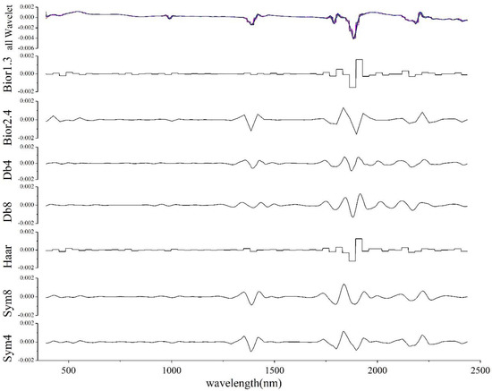
Figure 2.
Single branches reconstructed from the sixth-level discrete wavelet transform (DWT) approximate coefficients and fourth-level detailed coefficients of different wavelet functions.
With reference to previous studies, the predictive ability of the DWT–PLS and DWT–Stepwise-PLS method was assessed by four indicators: the coefficient of determination R2, the p value, root-mean-square deviation (RMSE), and the relative percentage deviation (RPD). R2 represented the calibration measures of the models, and Rv2, RMSE, and RPD represented the validation measures of the models. Along with the p value, R2 also evaluates the degree of correlation between the predicted and true values. As the RMSE is a parameter in the Stepwise-PLS model, it was excluded as an evaluation indicator of the model’s calibration results, but was added as an effective evaluation indicator of the model’s validation results. The RMSE and RPD define the accuracy of the error between the predicted and true values. Mathematically, RPD defines the ratio of the sample standard deviation (StD) to the RMSE (StD/RMSE). According to related research [36], models with RPD values below 1.0 are very poor predictive performers, and their use is not recommended. Models with RPD values between 1.0 and 1.4 are also poor performers, and can distinguish only high and low values. When the RPD values is between 1.4 and 1.8, the model is a fair performer, and is useful for assessment and correlation. Models with RPD values between 1.8 and 2.0 are sufficiently accurate for quantitative predictions, and those with RPD values between 2.0 and 2.5 are high-quality quantitative predictors. Any model with an RPD values above 2.5 makes excellent predictions.
Furthermore, in order to directly compare the DWT–PLS and DWT–Stepwise-PLS model, the difference between the R2 values of DWT–PLS and DWT–Stepwise-PLS were used to compare the model efficiencies, and were defined as the R2 D-value. Additionally, the difference between the RMSE of DWT–PLS and DWT–Stepwise-PLS were defined as the RMSE D-value. Some statistical parameters of RPD for DWT–PLS and DWT–Stepwise-PLS models are also calculated: the maximum value, minimum value, and average value of PRD at different decomposition levels of the same wavelet functions; and the difference (D-value) of PRD between DWT–Stepwise-PLS and DWT–PLS.
3. Results and Discussion
3.1. Characteristics of Soil Properties
Table 1 lists the maxima, minima, means, standard deviations (StD), and coefficients of variance (CV) of the soil properties. The soil densities (SD) of the soil samples vary between 0.64 and 1.53, and their average is 1.15 g/cm3. The StD and CV are both low (StD = 0.11; CV = 9.82). The soil samples cover alkaline, acidic, and neutral soils with pH levels between 9.56 and 3.25. The CEC of the soil samples range from 2.76 to 50.10, with StD and CV values of 7.97 and 40.71, respectively. Similarly, the SOM range from 1.34 to 44.38, with StD and CV of 7.70 and 52.93, respectively. Clearly, the densities and pH of soil samples have lower StD and CV values than the SOM and CEC.
Prior to spectral analysis, we must determine the intrinsic relationships between the soil density, pH, SOM, and CEC of the soils. The correlation coefficients between pairs of soil density, pH, SOM, and CEC values are shown in Table 4. There are no significant correlations between the soil properties, implying that these four indexes are individual and representative of the study area.
Table 4.
Pearson’s correlation coefficients (R) between soil properties for tested soil properties.
3.2. Reflectance Spectral Feature of Soil Properties
Panels (a) and (b) of Figure 3 show the average spectral reflectance of the soil samples and their first derivatives, respectively. The first derivatives of the soil reflectance contain more absorption bands, and hence much more SOM and CEC information than the raw average spectral reflectance. The absorption bands in the first derivatives appear near 566 nm, 1418 nm, 1918 nm, and 2205 nm.
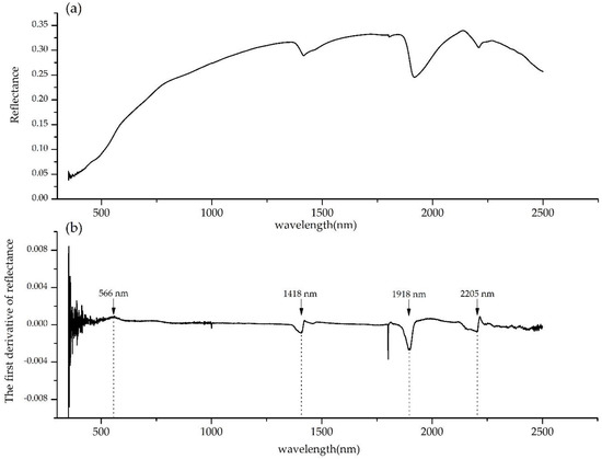
Figure 3.
Average reflectance spectra (a) and its first derivative (b).
Figure 4 plots the Pearson’s correlation coefficients between the first derivative of the reflection spectrum and the soil properties as functions of wavelength. As indicated in Figure 4, SOM has more absorption bands than CEC, with characteristic spectral peaks at 1388 nm, 1888 nm, 2182 nm, and 2303 nm for positive correlations, and with characteristic spectral peaks at 732 nm, 1257 nm, 1469 nm, and 2022 nm for negative correlations. Many of these absorption bands are immediately attributable to organic matter (such as absorptions by hydroxyl (O–H) stretching vibrations near 1469 nm and 1888 nm, and aliphatic C–H stretching near 2182 nm [15]). The absorption spectral bands of CEC appear at 710 nm, 1274 nm, 1442 nm, and 1966 nm (all negative correlations).
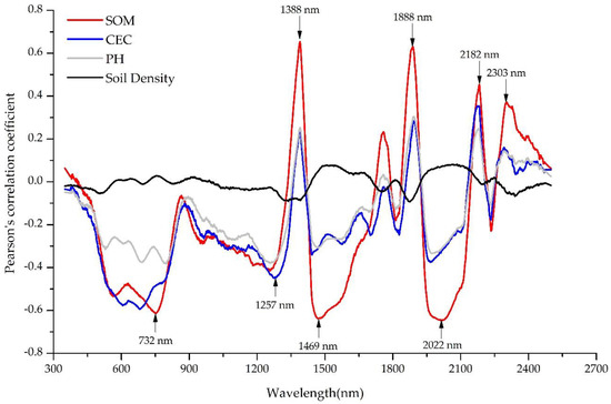
Figure 4.
Pearson’s correlation coefficients between the soil-reflection spectral bands and soil properties (soil organic matter (SOM), cation exchange capacity (CEC), pH, and soil density), as functions of wavelengths.
Obviously, the negatively-correlated absorption bands of the SOM and CEC are very similar, indicating that the characteristic reflection bands of the SOM and CEC probably overlap (masking effect). This masking effect of spectral features is common, which complicates the spectral analysis. Therefore, the classification of soil samples is necessary before analyzing the quantitative prediction model (Section 2.1).
According to the Table 2, the CVs of all soil properties (except CEC) are below 40%, indicating that the pH, soil density, and SOM exert limited impacts on the CEC in the spectral analysis. The StDs and CVs of the pH and soil density are very small, meaning that the variations in these properties (pH and soil density) are insufficient for effective modeling. Moreover, because of their small CV, their spectral features are easily covered by the SOM and CEC features (Figure 4). Hence, in the following discussion, the pH and soil density are treated only as simple comparison items, while the SOM and CEC (which are important indicators of soil fertility) are the main variables in the spectral analysis.
3.3. Regression Analysis Based on Discrete Wavelet Transform with Partial Least-Squares
3.3.1. Calibration of the Discrete Wavelet Transform with Partial Least-Squares Model
The calibration results of DWT–PLS are summarized in Table 5. The SOM and CEC prediction models established by DWT–PLS perform well on the calibration dataset in this study. Moreover, the DWT–PLS models perform better at levels 5, 6, 7, and 8 of the DWT than at levels 3 and 4, with a larger R2 (Table 5), meaning that higher decomposition levels improve the performance of the DWT–PLS model, which quantitatively predicts the SOM and CEC values. In the calibration set of the quantitative CEC prediction, the R2 values yielded by the DWT–PLS models using the Haar, Sym8, and Db4 wavelet functions were 0.97, 0.97, and 0.92, respectively (all > 0.90).
Table 5.
Coefficient of determination (R2) values and number of variables (N) used in discrete wavelet transform with partial least-squares (DWT–PLS) models for CEC and SOM in calibration set.
In the calibration set of the quantitative SOM prediction, the R2 values (again > 0.90) yielded by DWT–PLS models using the Bior2.4, Haar, Sym4, and Sym8 wavelet functions were 0.95, 0.91, 0.91, and 0.91, respectively. Table 5 also lists the number of variables used in the DWT–PLS models of the CEC and SOM predictions. Because the SOM spectrum has more absorption bands than the CEC spectrum (Figure 4), the coefficients of the DWT–PLS prediction model are generally more variable for SOM than for CEC.
3.3.2. Validation of the Discrete Wavelet Transform with Partial Least-Squares Model
The validation results of the DWT–PLS model are shown in Figure 5 and Figure 6. All wavelet functions used in the DWT–PLS model showed different prediction results for SOM and CEC. Among the DWT–PLS models for CEC prediction, DWT–PLS with the Haar wavelet function gave the highest Rv2, lowest RMSE, and highest RPD values (0.787, 4.16, and 2.047, respectively), meaning that the Haar wavelet function maximizes the performance of the DWT–PLS model in the validation dataset. Viscarra-Rossel [10] observed an R2 value (0.73) close to this study for CEC prediction in the Vis-NIR by PLS method; Pinheiro et al. [37] also observed similar R2 values (0.68), RMSE values (5.86), and RPD values (1.17) for CEC prediction in the Vis-NIR by PLS method. Moreover, the maximum RPD of DWT–PLS, regardless of wavelet function, is distributed around levels 5, 6, and 7, and remains relatively stable over those levels (Figure 5c). These results show the obvious advantages of levels 5, 6, and 7 over the other levels. According to previous studies [7], lower-level DWT coefficients introduce high-frequency noise that affects the model predictions; conversely, higher-level DWT coefficients filter much of the available spectral information, also decreasing the predictive ability of the model.
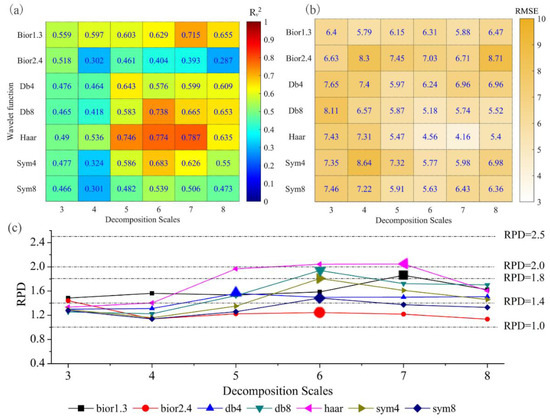
Figure 5.
Coefficients of determination (Rv2) (a), root mean square error (RMSE) (b) and relative percentage deviation (RPD) (c) between the laboratory-measured CECs and the DWT–PLS predictions on the CEC validation dataset.
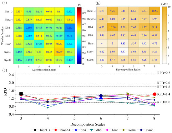
Figure 6.
Coefficients of determination (Rv2) (a), RMSE (b), and RPD (c) between the laboratory-measured SOMs and the DWT–PLS predictions on the SOM validation dataset.
As shown in Figure 5a and Figure 6a, the validation results of CEC are better overall than those of SOM. The RPD of the SOM predictions by DWT–PLS was maximized at 1.441 (Rv2 = 0.637, RMSE = 5.73), highlighting the poor overall predictive ability of SOM by DWT–PLS. Vohland et al. [38] also observed a similar R2 value, RMSE value, and RPD value (0.60, 0.41, and 1.58 respectively) for soil organic C prediction in the Vis-NIR by the PLSR method. The SOM predictions also lack the regularity of the CEC results with regard to the optimal decomposition-level distributions and the optimal wavelet functions in the DWT–PLS model. The SOM prediction model has more the variables of the DWT–PLS prediction model than the CEC (Table 5). This results are similar to the study results of Dunn et al. [39], who predicted CEC (R2 = 0.9, RPD = 3.3) with higher levels of accuracy than soil organic C (R2 = 0.66, RPD = 1.7) in the Vis-NIR by the PLS method. Although more variable factors capture more information from the soil reflectance spectra, increasing the number of variable factors in the DWT–PLS model unfortunately introduced more unreasonable variables into the regression equations, increasing the noise and errors.
3.4. Improved Model Using Discrete Wavelet Transform with Stepwise-Partial Least-Squares and Model Comparison
3.4.1. Calibration and Validation Results of the Discrete Wavelet Transform–Stepwise-Partial Least Squares Model
The DWT–Stepwise-PLS models for predicting CEC and SOM were calibrated on the same datasets used for calibrating their DWT–PLS counterparts, with no additional processing. The DWT–Stepwise-PLS model yielded a better calibration result than the DWT–PLS model; the R2 values of both models were very close to 1 (Table 6). Note that when comparing the DWT–PLS models, the numbers (N) of the variables are not significantly decreased in the DWT–Stepwise-PLS models with the same wavelet function and decomposition level (Table 5 and Table 6). This result implies that the DWT–Stepwise-PLS method selects more effective variables than DWT–PLS.
Table 6.
Coefficient of determination (R2) and number of variables (N) used in DWT–Stepwise-PLS models for CEC and SOM in the calibration set.
The validation results of the DWT–Stepwise-PLS models for CEC and SOM are shown in Figure 7 and Figure 8, respectively. The numbers in the grid are the Rv2 values of the DWT–Stepwise-PLS for validation datasets with various wavelet functions and decomposition levels (Figure 7a and Figure 8a). The fill colors of the grids represent the difference values (D-values) of Rv2 between the DWT–Stepwise-PLS and DWT–PLS methods. As the fill color approaches green (red), the D-values of the Rv2 between the DWT–Stepwise-PLS and DWT–PLS increase (decrease). Most of the grids are green or write, implying that the DWT–Stepwise-PLS method better predicts the SOM and CEC in soils than DWT–PLS with different wavelet functions and decomposition levels. Among the DWT–Stepwise-PLS models for CEC prediction, DWT–Stepwise-PLS with the Haar wavelet function gave the highest Rv2, RMSE, and RPD (0.92, 4.91, and 3.57, respectively). CEC was accurately predicted by DWT–Stepwise-PLS, and similar results have been reported in other studies [6,39]. DWT–Stepwise-PLS with the Bior2.4 wavelet function gave the highest Rv2, RMSE, and RPD (0.8., 5.34, and 2.24, respectively). These results are similar to the results of McCarty et al. [40], who observed close R2 values and RMSE values (0.82 and 5.5, respectively) for soil organic C prediction in the NIR by the PLSR method. Rossel et al. [10] also observed similar R2 values (R2 = 0.60) and RMSE values (RMSE = 0.18) in the visible reflectance and near-infrared reflectance for soil organic C prediction by the PLSR method.
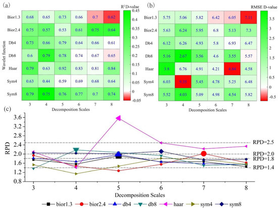
Figure 7.
Rv2 (numbers in grid squares) and R2 difference value (D-value) (color bar) between DWT–Stepwise-PLS and DWT–PLS (a), RMSE (numbers in grid squares) and RMSE D-value (color bar) between DWT–Stepwise-PLS and DWT–PLS (b), and RPD between the laboratory-measured CEC and the DWT–Stepwise-PLS predictions on the CEC validation data set (c).
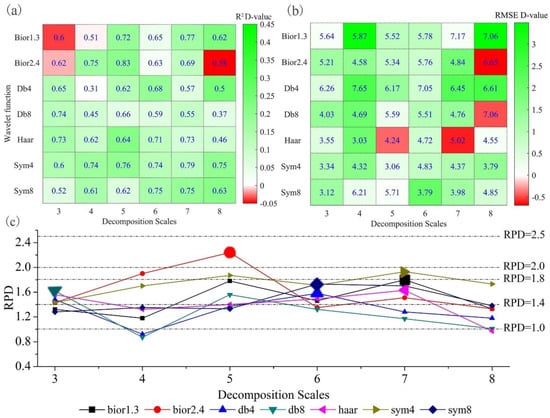
Figure 8.
Rv2 (numbers in grid squares) and R2 D-value (color bar) between DWT–Stepwise-PLS and DWT–PLS (a), RMSE (numbers in grid squares) and RMSE D-value (color bar) between DWT–Stepwise-PLS and DWT–PLS (b), and RPD between the laboratory-measured SOM and the DWT–Stepwise-PLS predictions on the SOM validation dataset (c).
3.4.2. Characteristics of Wavelet Functions Representativeness
The RPD values of the DWT–Stepwise-PLS at levels 3–8 are shown in Figure 7b and Figure 8b. The average RPD of the CEC predicted by DWT–Stepwise-PLS was higher for the Haar and Sym8 wavelet functions (2.36 and 1.96, respectively; see Table 7) than for the other wavelet functions. Moreover, according to the CEC validation results, the effect of DWT–Stepwise-PLS using the Haar and Sym8 wavelet functions largely depends on the decomposition level of the DWT; the former appears to be more effective at higher decomposition levels, whereas the latter tends to be relatively stable at each level (Figure 7b).
Table 7.
Statistical description of relative percent deviation (RPD) between DWT–Stepwise-PLS models and DWT–PLS models for CEC and SOM.
The average RPDs of the SOM predictions by DWT–Stepwise-PLS using Bior2.4 and Sym4 were 1.63 and 1.73, respectively (Table 7), showing slight advantages of Bior2.4 and Sym4 over the other wavelet functions. Similarly, most of the DWT–Stepwise-PLS models yielded higher Rv2 values than the DWT–PLS model (Figure 8). The DWT–Stepwise-PLS not only yielded a higher RPD with Sym4 than with Bior1.3, but was overall more stable with Sym4 than with the other wavelet functions.
3.5. Appropriateness of Discrete Wavelet Transform with Stepwise-Partial Least-Squares
The D-values of the maximum RPDs distributed around levels 5, 6, and 7 of the DWT–Stepwise-PLS model exceeded the D-values of both average and minimum RPDs of the model (Table 7), meaning that the low RPD values yielded by DWT–PLS are unlikely to be improved by Stepwise-PLS. Therefore, the appropriateness of the Stepwise-PLS is not greatly related to the RPD of the DWT–PLS predictions. Hence, we need to further explore whether the appropriateness is related to the level of wavelet decomposition.
Although most of the results demonstrate an obvious advantage of DWT–Stepwise-PLS over DWT–PLS, Stepwise-PLS reduces the prediction accuracy of CEC and SOM in isolated cases (Figure 7 and Figure 8). There are about 384 wavelet coefficients in the three-level wavelet decomposition of DWT (the exact number depends on the wavelet functions), revealing a significant amount of noise in the low-level decomposition wavelet coefficients. The noisy data are problematic for variable selection by the Stepwise-PLS method. The greater the number of variables, the more uncertain the Stepwise-PLS method will be. Nearly 136 wavelet coefficients were generated, mainly consisting of the approximated fourth-level signals and the detailed signals of the eighth-level decomposition. In the overall validation results of CEC and SOM, the performance of Stepwise-PLS is degraded in the seventh and eighth levels of Bior1.3 for the CEC prediction, in the first level of Bior1.3 and Bior2.4, and in the 7th level of Bior2.4 for the SOM prediction (Figure 7a and Figure 8a). Negative effects in the Stepwise-PLS method appear when the decomposition level is low or high, indicating that high-level wavelet decomposition over-compresses the spectral information. Therefore, inaccuracies in the Stepwise-PLS method may arise from the screening of useless information. In the case of fewer variables, the negative effect of this useless screening becomes significant.
This study explored the visible and near infrared reflectance analysis (Vis-NIRA) technique for estimating soil properties. In the future, the development of a software package would be more helpful for researchers who are interested in retrieving the large-scale soil properties, as was the case in our study. In our current research, we mainly focused on CEC and SOM by visible and near infrared reflectance analysis. However, other soil properties are still challenging, which needs more efforts in further research.
4. Conclusions
This study compared the appropriateness of inserting different wavelet functions with different decomposition levels in the discrete wavelet transform with partial least-squares (DWT–PLS) method into the conventional visible and near infrared reflectance analysis method for estimating soil properties. The reliability and accuracy of the soil properties estimated by discrete wavelet transform-based visible and near infrared reflectance analysis was enhanced by an improved partial least-squares method called Stepwise-PLS. The main conclusions of this study are summarized below:
(1) In a feasibility study, the discrete wavelet transform with partial least-squares method was applied to the quantitative analysis of soil properties. Varying the wavelet functions and their distribution levels, we found that the fifth, sixth and seventh levels of the Haar wavelet function benefitted from the discrete wavelet transform with partial least-squares estimation of cation exchange capacity, maximizing the R2 and RPD values. However, no wavelet function showed a clear advantage over the other functions in the discrete wavelet transform with partial least-squares method estimation of soil organic matter.
(2) The discrete wavelet transform with stepwise-partial least squares method, with various wavelet functions and decomposition levels, effectively improved the prediction accuracy of the cation exchange capacity and soil organic matter estimated by the Vis-NIRA method. Further analysis of the results confirmed that the appropriateness of discrete wavelet transform with stepwise-partial least-squares method is not significantly related to the RPD values of the predicted soil properties, but improves at the fifth, sixth, and seventh levels of the DWT. Therefore, the Stepwise-PLS method will more likely obtain poorer results at lower and higher decomposition levels than at intermediate-to moderately-high levels.
Author Contributions
Conceptualization: B.X. and G.W.; Methodology: W.W. and Q.F.; Formal Analysis: W.W., H.J., and Q.X.; Writing (Original Draft Preparation): G.W. and W.W.; Writing (Review and Editing): B.X.
Acknowledgments
This study was supported by the National Natural Science Foundation of China (Grant No. 51679006, 51779007 and 31670451), the Chinese National Special Science and Technology Program of Water Pollution Control and Treatment (No. 2017ZX07302-004), the Evaluation of Resources–Environmental Carrying Capacity in Typical Ecological Zones of Xinganling (Grant No. 12120115051201), the Fundamental Research Funds for the Central Universities (No. 2017NT18), and Key Projects for Young Teachers at Sun Yat-sen University (Grant No. 17lgzd02).
Conflicts of Interest
The authors declare no conflict of interest.
References
- Karlen, D.L.; Mausbach, M.J.; Doran, J.W.; Cline, R.G.; Harris, R.F.; Schuman, G.E. Soil quality: A concept, definition, and framework for evaluation (a guest editorial). Soil Sci. Soc. Am. J. 1997, 61, 4–10. [Google Scholar] [CrossRef]
- Nanni, M.R.; Demattê, J.A.M. Spectral reflectance methodology in comparison to traditional soil analysis. Soil Sci. Soc. Am. J. 2006, 70, 393–407. [Google Scholar] [CrossRef]
- Jung, W.K.; Kitchen, N.R.; Sudduth, K.A.; Anderson, S.H. Spatial characteristics of claypan soil properties in an agricultural field mention of trade names or commercial products is solely for the purpose of providing specific information and does not imply recommendation or endorsement by the u.S. Department of agriculture. Soil Sci. Soc. Am. J. 2006, 70, 1387–1397. [Google Scholar] [CrossRef]
- Alrajehy, A.M. Relationships between Soil Reflectance and Soil Physical and Chemical Properties. Ph.D. Thesis, Mississippi State University, Starkville, MS, USA, 2002. [Google Scholar]
- Ben-Dor, E.; Banin, A. Near infrared analysis (nira) as a method to simultaneously evaluate spectral featureless constituents in soils. Soil Sci. 1995, 159, 259–270. [Google Scholar] [CrossRef]
- Chang, C.-W.; Laird, D.A.; Mausbach, M.J.; Hurburgh, C.R. Near-infrared reflectance spectroscopy–principal components regression analyses of soil properties. Soil Sci. Soc. Am. J. 2001, 65, 480–490. [Google Scholar] [CrossRef]
- Ge, Y.; Thomasson, J.A. Wavelet incorporated spectral analysis for soil property determination. Trans. ASABE 2006, 49, 1193–1201. [Google Scholar] [CrossRef]
- Luleva, M.I.; Van der Werff, H.; Jetten, V.; Van der Meer, F. Can infrared spectroscopy be used to measure change in potassium nitrate concentration as a proxy for soil particle movement? Sensors 2011, 11, 4188. [Google Scholar] [CrossRef] [PubMed]
- Wetterlind, J.; Stenberg, B. Near-infrared spectroscopy for within-field soil characterization: Small local calibrations compared with national libraries spiked with local samples. Eur. J. Soil Sci. 2010, 61, 823–843. [Google Scholar] [CrossRef]
- Viscarra Rossel, R.A.; Walvoort, D.J.J.; McBratney, A.B.; Janik, L.J.; Skjemstad, J.O. Visible, near infrared, mid infrared or combined diffuse reflectance spectroscopy for simultaneous assessment of various soil properties. Geoderma 2006, 131, 59–75. [Google Scholar] [CrossRef]
- Knadel, M.; Gislum, R.; Hermansen, C.; Peng, Y.; Moldrup, P.; de Jonge, L.W.; Greve, M.H. Comparing predictive ability of laser-induced breakdown spectroscopy to visible near-infrared spectroscopy for soil property determination. Biosyst. Eng. 2017, 156, 157–172. [Google Scholar] [CrossRef]
- Wang, G.; Fang, Q.; Wu, B.; Yang, H.; Xu, Z. Relationship between soil erodibility and modeled infiltration rate in different soils. J. Hydrol. 2015, 528, 408–418. [Google Scholar] [CrossRef]
- Bruce, L.M.; Koger, C.H.; Li, J. Dimensionality reduction of hyperspectral data using discrete wavelet transform feature extraction. IEEE Trans. Geosci. Remote Sens. 2002, 40, 2331–2338. [Google Scholar] [CrossRef]
- Lark, R.; Webster, R. Analysis and elucidation of soil variation using wavelets. Eur. J. Soil Sci. 1999, 50, 185–206. [Google Scholar] [CrossRef]
- Viscarrarossel, R.A.; Lark, R.M. Improved analysis and modelling of soil diffuse reflectance spectra using wavelets. Eur. J. Soil Sci. 2009, 60, 453–464. [Google Scholar] [CrossRef]
- Wang, G.; Fang, Q.; Teng, Y.; Yu, J. Determination of the factors governing soil erodibility using hyperspectral visible and near-infrared reflectance spectroscopy. Int. J. Appl. Earth Obs. Geoinform. 2016, 53, 48–63. [Google Scholar] [CrossRef]
- Liu, H.; Shi, T.; Chen, Y.; Wang, J.; Fei, T.; Wu, G. Improving spectral estimation of soil organic carbon content through semi-supervised regression. Remote Sens. 2017, 9, 29. [Google Scholar] [CrossRef]
- Viscarra Rossel, R.A.; Behrens, T.; Ben-Dor, E.; Brown, D.J.; Demattê, J.A.M.; Shepherd, K.D.; Shi, Z.; Stenberg, B.; Stevens, A.; Adamchuk, V.; et al. A global spectral library to characterize the world’s soil. Earth-Sci. Rev. 2016, 155, 198–230. [Google Scholar] [CrossRef]
- Farifteh, J.; Van der Meer, F.; Atzberger, C.; Carranza, E.J.M. Quantitative analysis of salt-affected soil reflectance spectra: A comparison of two adaptive methods (plsr and ann). Remote Sens. Environ. 2007, 110, 59–78. [Google Scholar] [CrossRef]
- Rossel, R.A.V.; Behrens, T. Using data mining to model and interpret soil diffuse reflectance spectra. Geoderma 2010, 158, 46–54. [Google Scholar] [CrossRef]
- Shepherd, K.D.; Walsh, M.G. Development of reflectance spectral libraries for characterization of soil properties. Soil Sci. Soc. Am. J. 2002, 66, 988–998. [Google Scholar] [CrossRef]
- Vasques, G.M.; Grunwald, S.; Sickman, J.O. Comparison of multivariate methods for inferential modeling of soil carbon using visible/near-infrared spectra. Geoderma 2008, 146, 14–25. [Google Scholar] [CrossRef]
- Yu, X.; Liu, Q.; Wang, Y.; Liu, X.; Liu, X. Evaluation of mlsr and plsr for estimating soil element contents using visible/near-infrared spectroscopy in apple orchards on the jiaodong peninsula. CATENA 2016, 137, 340–349. [Google Scholar] [CrossRef]
- Stenberg, B.; Viscarra Rossel, R.A.; Mouazen, A.M.; Wetterlind, J. Chapter five—Visible and near infrared spectroscopy in soil science. In Advances in Agronomy; Sparks, D.L., Ed.; Academic Press: Cambridge, MA, USA, 2010; Volume 107, pp. 163–215. ISBN 0065-2113. [Google Scholar]
- Martens, H.; Geladi, P. Multivariate Calibration; Wiley Online Library: Hoboken, NJ, USA, 1989; ISBN 0471667196. [Google Scholar]
- Xiaobo, Z.; Jiewen, Z.; Povey, M.J.W.; Holmes, M.; Hanpin, M. Variables selection methods in near-infrared spectroscopy. Anal. Chim. Acta 2010, 667, 14–32. [Google Scholar] [CrossRef] [PubMed]
- Vohland, M.; Besold, J.; Hill, J.; Fründ, H.-C. Comparing different multivariate calibration methods for the determination of soil organic carbon pools with visible to near infrared spectroscopy. Geoderma 2011, 166, 198–205. [Google Scholar] [CrossRef]
- Andries, J.P.; Vander, H.Y.; Buydens, L.M. Improved variable reduction in partial least squares modelling based on predictive-property-ranked variables and adaptation of partial least squares complexity. Anal. Chim. Acta 2011, 705, 292–305. [Google Scholar] [CrossRef] [PubMed]
- Nocita, M.; Stevens, A.; Toth, G.; Panagos, P.; van Wesemael, B.; Montanarella, L. Prediction of soil organic carbon content by diffuse reflectance spectroscopy using a local partial least square regression approach. Soil Biol. Biochem. 2014, 68, 337–347. [Google Scholar] [CrossRef]
- Shi, T.; Chen, Y.; Liu, H.; Wang, J.; Wu, G. Soil organic carbon content estimation with laboratory-based visible–near-infrared reflectance spectroscopy: Feature selection. Appl. Spectrosc. 2014, 68, 831–837. [Google Scholar] [CrossRef] [PubMed]
- Institute of Soil Science, Chinese Academy of Sciences(I.S.S.C.A.S.). Physical and Chemical Analysis of Soil; Shanghai Scientific and Technical Publishers: Shanghai, China, 1978. [Google Scholar]
- Conforti, M.; Buttafuoco, G.; Leone, A.P.; Aucelli, P.P.C.; Robustelli, G.; Scarciglia, F. Studying the relationship between water-induced soil erosion and soil organic matter using vis-nir spectroscopy and geomorphological analysis: A case study in southern italy. Catena 2013, 110, 44–58. [Google Scholar] [CrossRef]
- Savitzky, A.; Golay, M.J.E. Smoothing and differentiation of data by simplified least squares procedures. Anal. Chem. 1964, 36, 1627–1639. [Google Scholar] [CrossRef]
- Krishnan, P.; Alexander, J.D.; Butler, B.J.; Hummel, J.W. Reflectance technique for predicting soil organic matter. Soil Sci. Soc. Am. J. 1980, 44, 1282–1285. [Google Scholar] [CrossRef]
- Mallat, S.G. A theory for multiresolution signal decomposition: The wavelet representation. IEEE Trans. Pattern Anal. Mach. Intell. 1989, 11, 674–693. [Google Scholar] [CrossRef]
- Viscarra Rossel, R.A.; McGlynn, R.N.; McBratney, A.B. Determining the composition of mineral-organic mixes using uv–vis–nir diffuse reflectance spectroscopy. Geoderma 2006, 137, 70–82. [Google Scholar] [CrossRef]
- Pinheiro, É.; Ceddia, M.; Clingensmith, C.; Grunwald, S.; Vasques, G. Prediction of soil physical and chemical properties by visible and near-infrared diffuse reflectance spectroscopy in the central amazon. Remote Sens. 2017, 9, 293. [Google Scholar] [CrossRef]
- Vohland, M.; Ludwig, M.; Thiele-Bruhn, S.; Ludwig, B. Determination of soil properties with visible to near- and mid-infrared spectroscopy: Effects of spectral variable selection. Geoderma 2014, 223–225, 88–96. [Google Scholar] [CrossRef]
- Dunn, B.W.; Beecher, H.G.; Batten, G.D.; Ciavarella, S. The potential of near-infrared reflectance spectroscopy for soil analysis—A case study from the riverine plain of south-eastern australia. Aust. J. Exp. Agric. 2002, 42, 607–614. [Google Scholar] [CrossRef]
- McCarty, G.W.; Reeves, J.B.; Reeves, V.B.; Follett, R.F.; Kimble, J.M. Mid-infrared and near-infrared diffuse reflectance spectroscopy for soil carbon measurement. Soil Sci. Soc. Am. J. 2002, 66, 640–646. [Google Scholar] [CrossRef]
© 2018 by the authors. Licensee MDPI, Basel, Switzerland. This article is an open access article distributed under the terms and conditions of the Creative Commons Attribution (CC BY) license (http://creativecommons.org/licenses/by/4.0/).